Uncertainty Analysis of Two Copula-Based Conditional Regional Design Flood Composition Methods: A Case Study of Huai River, China

 , ,
, ,
Abstract
:1. Introduction
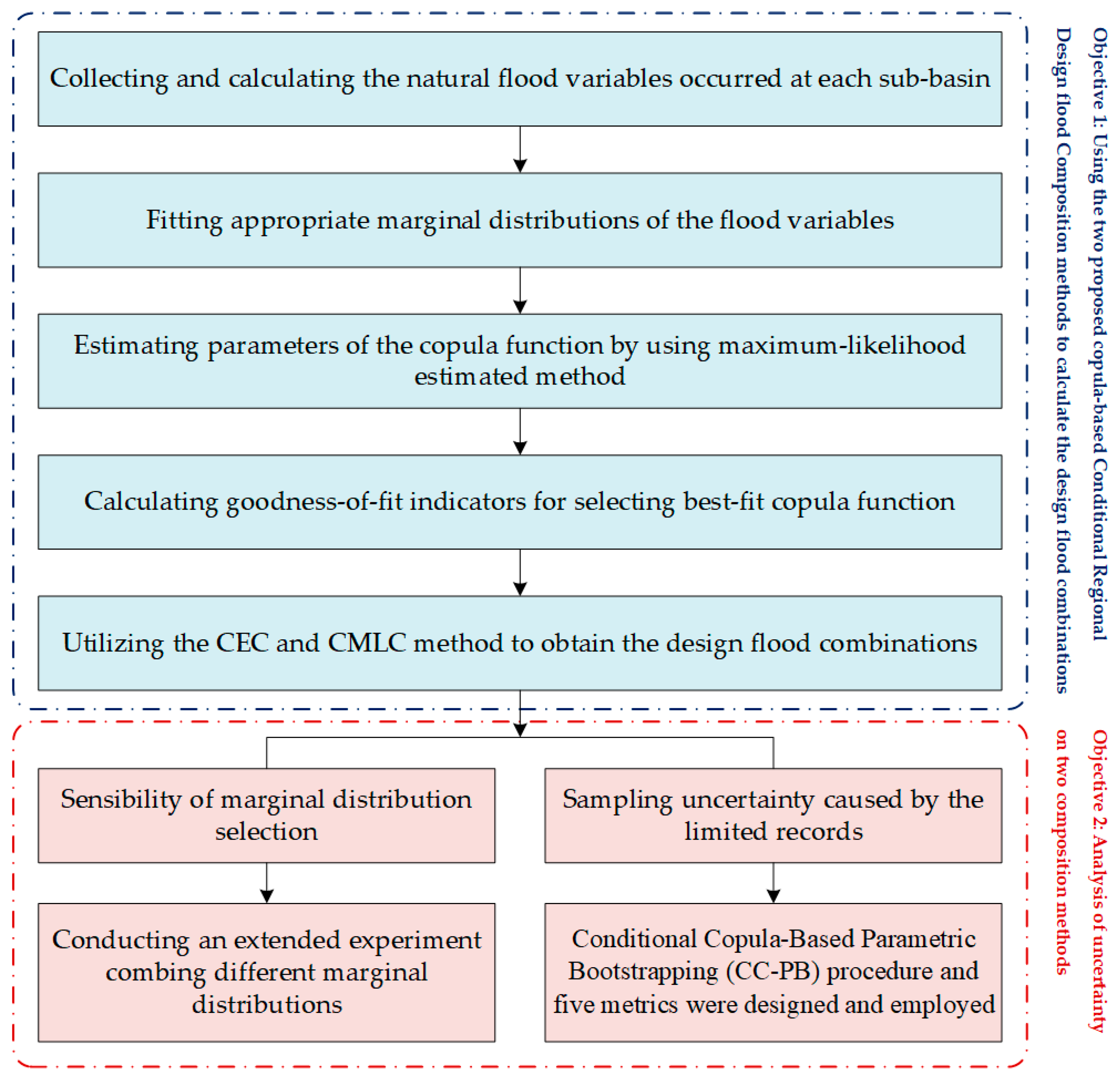
2. Methodology
2.1. Copula Theory
2.2. Regional Design Flood Composition
2.2.1. Basic Concept of Regional Design Flood Composition
2.2.2. Flood Regional Composition Methods Based on Copulas
2.3. Conditional Copula-Based Parametric Bootstrapping (CC-PB) Procedure
- Fit the marginal distributions and parametric copula function for the original dataset (i.e., X and Y). The parameters of the chosen marginal distributions and copula function are estimated by the L-moment method and maximum pseudo-log-likelihood (ML) method, respectively.
- Predefine NB bivariate bootstrapping samplings of size n through the usage of the conditional simulation method [29], and then obtain Z* = (X*,Y*) = (xij,yij) from the bivariate dependence structure via the probability integral transform (PIT) using the fitted parameters of the margins (i = 1,…,n; j = 1,…,NB).
- Estimate the parameters of marginal distributions and the parametric copula function of Z* utilizing the same estimation method used for the original dataset, then obtain NB pairs of Fj*(xij,yij), (i = 1,…,n; j = 1,…,NB).
- Identify the CEC and CMLC realizations for different (x,y) pairs by Equations (2) and (4), respectively.
- Utilize these realizations to estimate the bivariate confidence intervals (BCIs) by employing the kernel density estimation (KDE) method [34].
2.4. Metrics for Sampling Uncertainty
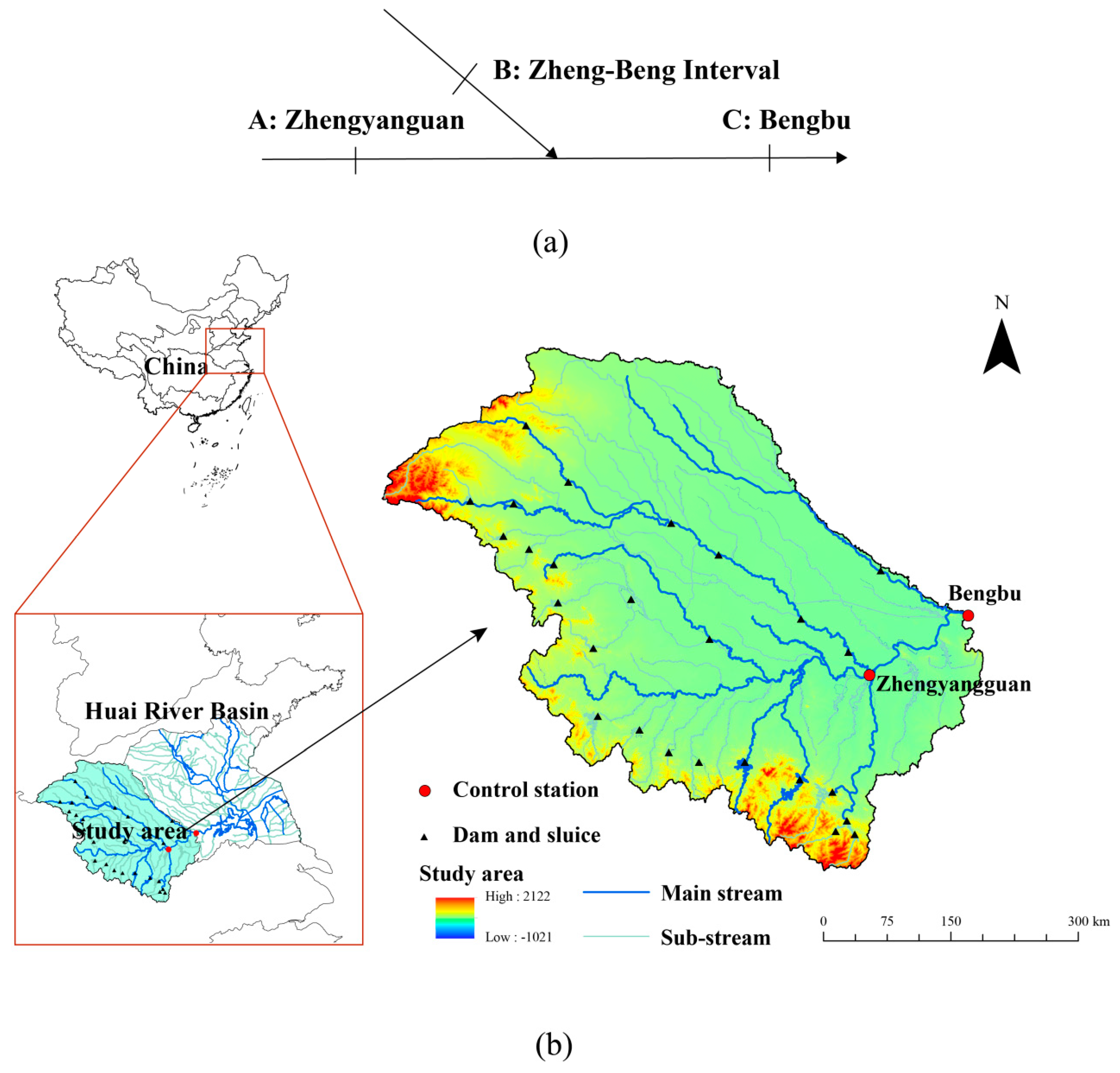
3. Study Area and Data
4. Results and Discussions
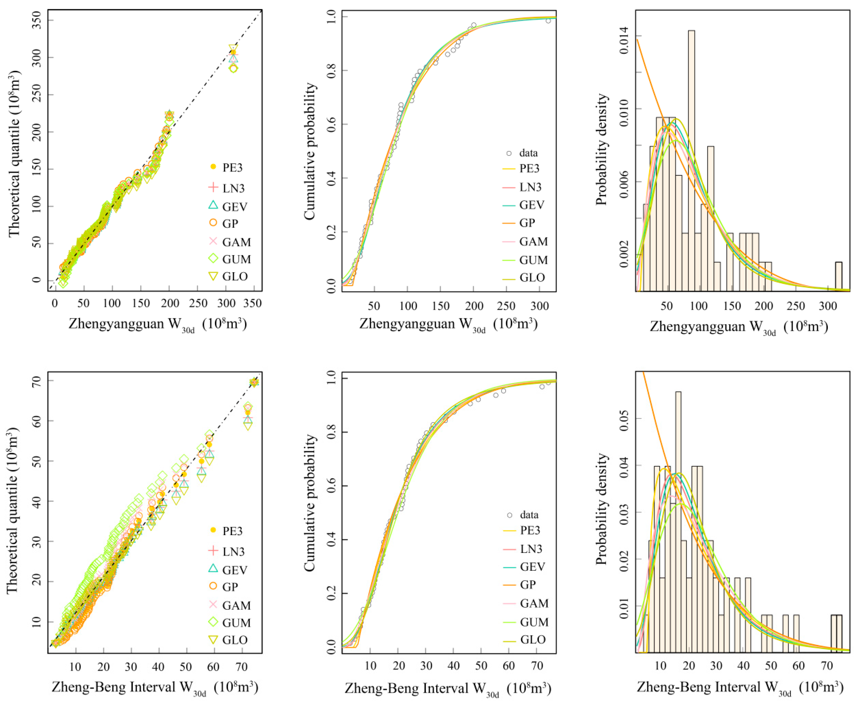
4.1. Selection of Marginal Distribution
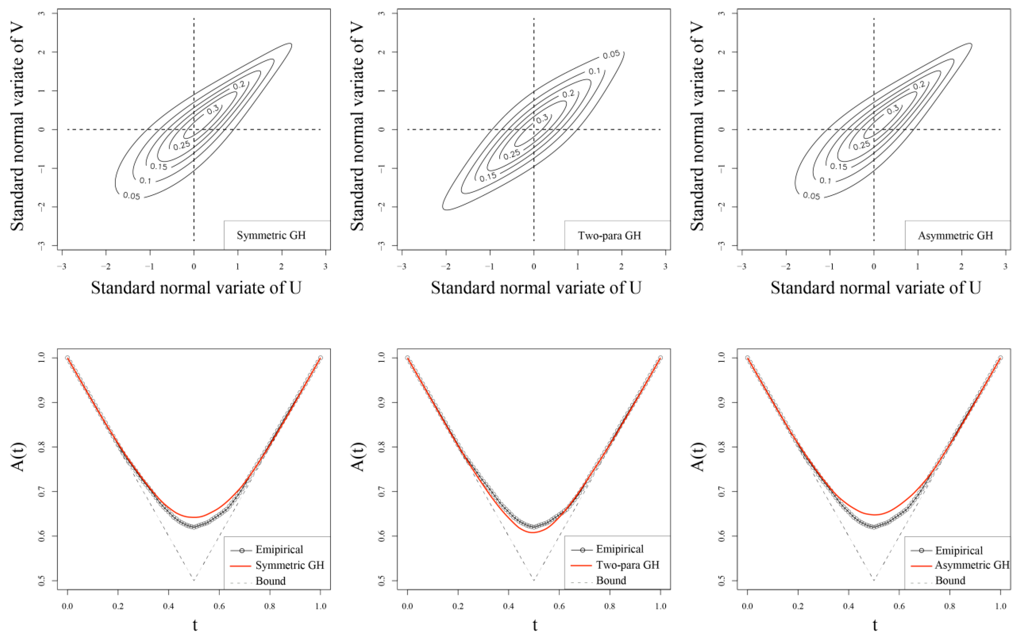
4.2. Copula Function Construction
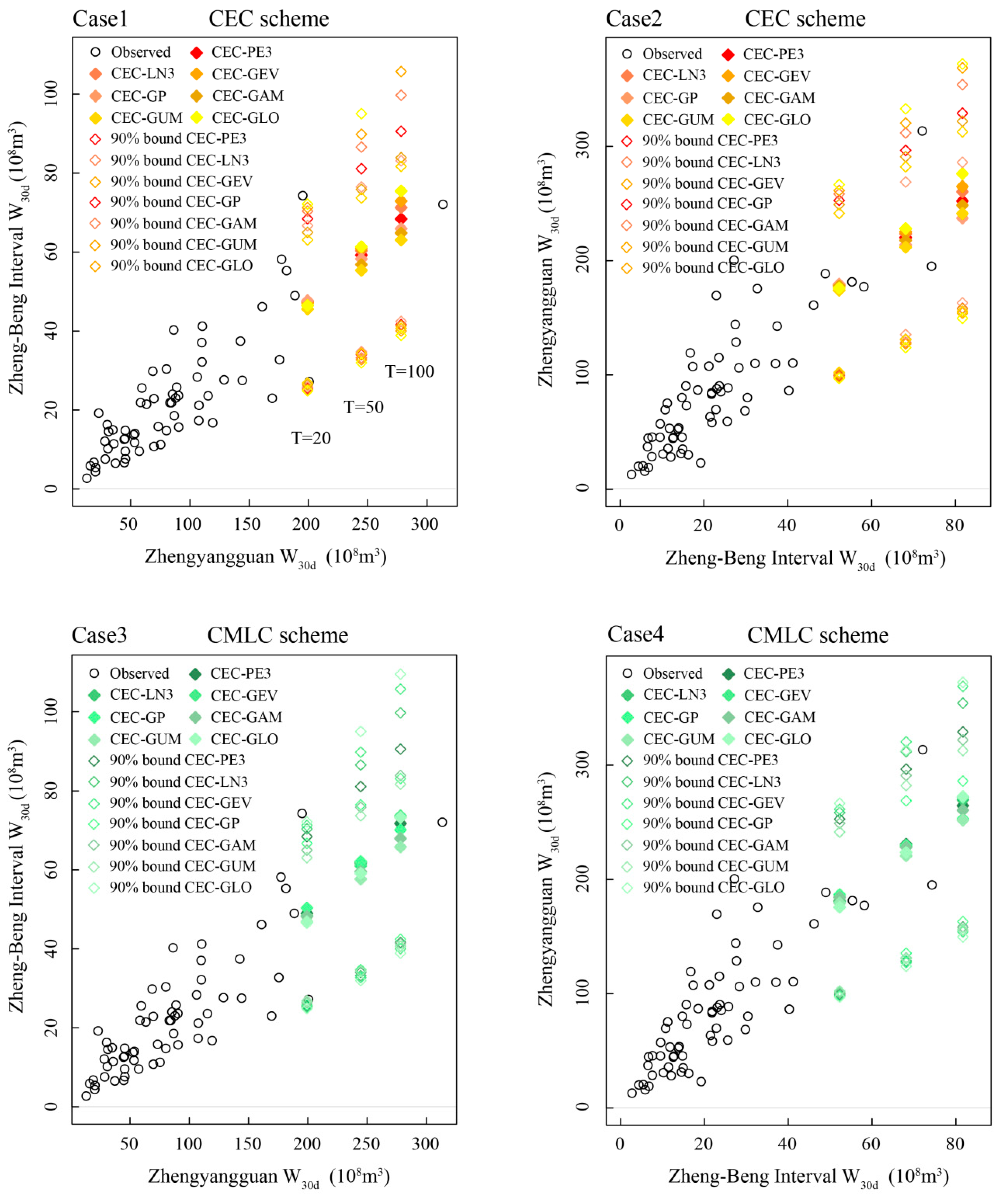
4.3. CEC and CMLC Point Identification
4.4. Uncertainty Analysis
4.4.1. Uncertainty Due to the Selection of Margins
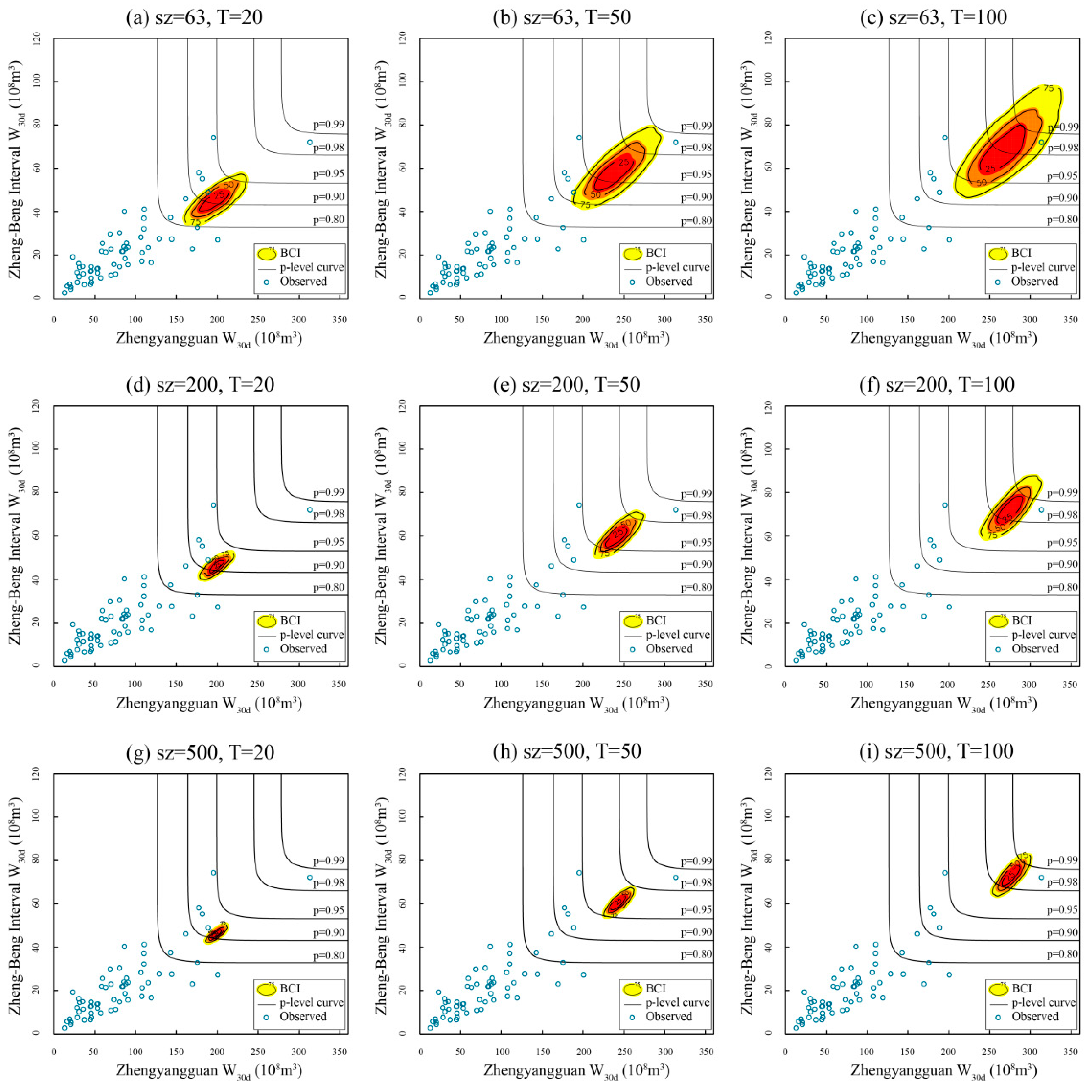
4.4.2. Sampling Uncertainty Caused by the Limited Records
- Three values of T for the W30d at two sub-basins, respectively, are selected (viz., T = 20, 50, 100 years), ranging from the moderate flood volume standard to the extreme one. Similarly, three values of sample size (sz) are selected (viz., sz = 63, 200, 500).
- Here, the selected model combination is C3, listed in Table 5. The CEC and CMLC events for C3 are estimated by fixing the value of sz (or T), and leaving the other variable vary in the corresponding subset. A triple of BCIs (viz., 25%, 50%, 75%) is exhibited under different schemes (sz, T). The larger the BCIs, the greater the uncertainty, and vice versa.
- To judge the plausibility and compare the performance of the two proposed composition methods, the contours of several selected joint probability levels [11] (viz., p-level = 0.99, 0.98, 0.95, 0.90, 0.80) together with the observed data are plotted on the same graphs as a reference.
- Five indexes mentioned above are also calculated (Table 7) to evaluate the sampling uncertainty of the 36 schemes.
5. Conclusions
Author Contributions
Funding
Conflicts of Interest
References
- Maidment, D.R. Handbook of Hydrology; McGraw-Hill: New York, NY, USA, 1993. [Google Scholar]
- Kendall, M.G. The advanced theory of statistics. Technometrics 1963, 5, 525–528. [Google Scholar]
- Lu, B.H.; Gu, H.H.; Xie, Z.Y.; Liu, J.F.; Ma, L.J.; Lu, W.X. Stochastic simulation for determining the design flood of cascade reservoir systems. Hydrol. Res. 2012, 43, 54–63. [Google Scholar] [CrossRef]
- De Michele, C.; Salvadori, G. A Generalized Pareto intensity-duration model of storm rainfall exploiting 2-Copulas. J. Geophys. Res. 2003, 108. [Google Scholar] [CrossRef] [Green Version]
- Favre, A.C.; El Adlouni, S.; Perreault, L.; Thiemonge, N.; Bobee, B. Multivariate hydrological frequency analysis using copulas. Water Resour. Res. 2004, 40. [Google Scholar] [CrossRef] [Green Version]
- Grimaldi, S.; Serinaldi, F. Asymmetric copula in multivariate flood frequency analysis. Adv. Water Resour. 2006, 29, 1155–1167. [Google Scholar] [CrossRef]
- Zhang, T.; Wang, Y.; Wang, B.; Tan, S.; Feng, P. Nonstationary Flood Frequency Analysis Using Univariate and Bivariate Time-Varying Models Based on GAMLSS. Water 2018, 10, 819. [Google Scholar] [CrossRef]
- Gu, H.; Yu, Z.; Li, G.; Ju, Q. Nonstationary Multivariate Hydrological Frequency Analysis in the Upper Zhanghe River Basin, China. Water 2018, 10, 772. [Google Scholar] [CrossRef]
- Salvadori, G.; Michele, C.D. Multivariate real-time assessment of droughts via copula-based multi-site Hazard Trajectories and Fans. J. Hydrol. 2015, 526, 101–115. [Google Scholar] [CrossRef]
- De Luca, D.L.; Biondi, D. Bivariate Return Period for Design Hyetograph and Relationship with T-Year Design Flood Peak. Water 2017, 9, 673. [Google Scholar] [CrossRef]
- Serinaldi, F. Dismissing return periods! Stoch. Environ. Res. Risk A 2015, 29, 1179–1189. [Google Scholar] [CrossRef]
- Amir, A.K.; András, B.R.; Emad, H. Copula-based uncertainty modelling: Application to multisensor precipitation estimates. Hydrol. Process 2010, 24, 2111–2124. [Google Scholar]
- Wang, W.; Dong, Z.; Zhu, F.; Cao, Q.; Chen, J.; Yu, X. A Stochastic Simulation Model for Monthly River Flow in Dry Season. Water 2018, 10, 1654. [Google Scholar] [CrossRef]
- Wang, Y.; Liu, G.; Guo, E.; Yun, X. Quantitative Agricultural Flood Risk Assessment Using Vulnerability Surface and Copula Functions. Water 2018, 10, 1229. [Google Scholar] [CrossRef]
- Zhao, P.; Lü, H.; Fu, G.; Zhu, Y.; Su, J.; Wang, J. Uncertainty of Hydrological Drought Characteristics with Copula Functions and Probability Distributions: A Case Study of Weihe River, China. Water 2017, 9, 334. [Google Scholar] [CrossRef]
- Salvadori, G.; Michele, C.D.; Durante, F. Multivariate design via Copulas. Hydrol. Earth Syst. Sci. 2011, 8, 5523–5558. [Google Scholar] [CrossRef]
- Volpi, E.; Fiori, A. Design event selection in bivariate hydrological frequency analysis. Hydrol. Sci. J. 2012, 57, 1506–1515. [Google Scholar] [CrossRef] [Green Version]
- Li, T.; Guo, S.; Liu, Z.; Xiong, L.; Yin, J. Bivariate design flood quantile selection using copulas. Hydrol. Res. 2016, 48. [Google Scholar] [CrossRef]
- Yan, B.W.; Guo, S.L.; Guo, J.; Chen, L.; Liu, P.; Chen, H. Regional design flood composition based on Copula function. J. Hydroelectr. Eng. 2010, 29, 60–65. (In Chinese) [Google Scholar]
- Liu, Z.; Guo, S.; Li, T.; Xu, C. General formula derivation of most likely regional composition method for design flood estimation of cascade reservoirs system. Adv. Water Sci. 2014, 25, 575–584. [Google Scholar]
- Li, T.; Guo, S.; Liu, Z.; Xu, C. Design flood estimation methods for cascade reservoirs. J. Hydraul. Eng. 2014, 1, 641–648. [Google Scholar]
- Ministry of Water Resources (MWR). Guidelines for Calculating Design Flood of Water Resources and Hydropower Projects; Chinese Water Resources and Hydropower Press: Beijing, China, 2006. (In Chinese)
- Guo, S.; Muhammad, R.; Liu, Z.; Xiong, F.; Yin, J. Design Flood Estimation Methods for Cascade Reservoirs Based on Copulas. Water 2018, 10, 560. [Google Scholar] [CrossRef]
- Serinaldi, F. An uncertain journey around the tails of multivariate hydrological distributions. Water Resour. Res. 2013, 49, 6527–6547. [Google Scholar] [CrossRef] [Green Version]
- Dung, N.V.; Merz, B.; Bárdossy, A.; Apel, H. Handling uncertainty in bivariate quantile estimation—An application to flood hazard analysis in the Mekong Delta. J. Hydrol. 2015, 527, 704–717. [Google Scholar] [CrossRef]
- Serinaldi, F.; Kilsby, C.G. Stationarity is undead: Uncertainty dominates the distribution of extremes. Adv. Water Resour. 2015, 77, 17–36. [Google Scholar] [CrossRef]
- Sklar, M. Fonctions de repartition a n dimensions et leurs marges. Publ. Inst. Stat. Univ. Paris 1959, 8, 229–231. [Google Scholar]
- Nelsen, R.B. An Introduction to Copulas. Technometrics 2000, 42, 317. [Google Scholar]
- Salvadori, G.; Michele, C.D.; Kottegoda, N.T.; Rosso, R. Extremes in Nature: An Approach Using Copulas; SpringerScience & Business Media: Berlin, Germany, 2007. [Google Scholar]
- Chebana, F. Copula representation of bivariate-moments: A new estimation method for multiparameter two-dimensional copula models. Statistics 2011, 49, 497–521. [Google Scholar]
- Joe, H. Dependence Modeling with Copulas; CRC Press: Boca Raton, FL, USA, 2014. [Google Scholar]
- Onyutha, C. On Rigorous Drought Assessment Using Daily Time Scale: Non-Stationary Frequency Analyses, Revisited Concepts, and a New Method to Yield Non-Parametric Indices. Hydrology 2017, 4, 48. [Google Scholar] [CrossRef]
- Al-Baali, M.; Purnama, A. Numerical Optimization; Springer: New York, NY, USA, 1999; pp. 29–76. [Google Scholar]
- Duong, T. KS: Kernel density estimation and kernel discriminant analysis for multivariate data in R. J. Stat. Softw. 2007, 21, 1–16. [Google Scholar] [CrossRef]
- Yin, J.; Guo, S.; Liu, Z.; Yang, G.; Zhong, Y.; Liu, D. Uncertainty Analysis of Bivariate Design Flood Estimation and its Impacts on Reservoir Routing. Water Resour. Manag. 2018, 32, 1795–1809. [Google Scholar] [CrossRef]
- Zhang, Y.Y.; Xia, J.; Liang, T.; Shao, Q.X. Impact of Water Projects on River Flow Regimes and Water Quality in Huai River Basin. Water Resour. Manag. 2010, 24, 889–908. [Google Scholar] [CrossRef]
- Ministry of Water Resources(MWR). Design Flood Calculation Regulating for Water Resources and Hydropower Engineering (SL44-2006); Chinese Water Resources and Hydropower Press: Beijing, China, 2006. (In Chinese)
- Gill, M.A. Flood routing by the Muskingum method. J. Hydrol. 1978, 36, 353–363. [Google Scholar] [CrossRef]
- Singh, V.P.; Rajagopal, A.K.; Singh, K. Derivation of some frequency distributions using the principle of maximum entropy (POME). Adv. Water Resour. 1986, 9, 91–106. [Google Scholar] [CrossRef]
- Hosking, J.R.M.; Wallis, J.R. Regional Frequency Analysis; Cambridge University Press: Cambridge, UK, 1997. [Google Scholar]
- Akaike, H. Information theory and an extension of the maximum likelihood principle. Int. Symp. Inf. Theory 1973, 267–281. [Google Scholar]
- Lariccia, V.; Mason, D.M. Cramér-von Mises statistics based on the sample quantile function and estimated parameters. J. Multivar. Anal. 1986, 18, 93–106. [Google Scholar] [CrossRef]
- Frahm, G.; Junker, M.; Schmidt, R. Estimating the tail-dependence coefficient: Properties and pitfalls. Insur. Math. Econ. 2005, 37, 80–100. [Google Scholar] [CrossRef]
- Genest, C.; Segers, J. Rank-Based Inference for Bivariate Extreme-Value Copulas. Ann. Stat. 2009, 37, 2990–3022. [Google Scholar] [CrossRef]
- Guo, A.; Chang, J.; Wang, Y.; Huang, Q.; Guo, Z. Maximum Entropy-Copula Method for Hydrological Risk Analysis under Uncertainty: A Case Study on the Loess Plateau, China. Entropy 2017, 19, 609. [Google Scholar] [CrossRef]
- Merz, R.; Blöschl, G.N. Flood frequency hydrology: 1. Temporal, spatial, and causal expansion of information. Water Resour. Res. 2008, 44, 8432. [Google Scholar] [CrossRef]


| Name | Descriptions |
|---|---|
| Symmetric GH copula | |
| Two-para GH copula | |
| Asymmetric GH copula | |
| u∈[0, 1], v∈[0, 1] : Copula parameter C: Copula function A: Marshall-Olkin copulas |
| Zhengyangguan W30d (108 m3) | Zheng-Beng Interval W30d (108 m3) | |
|---|---|---|
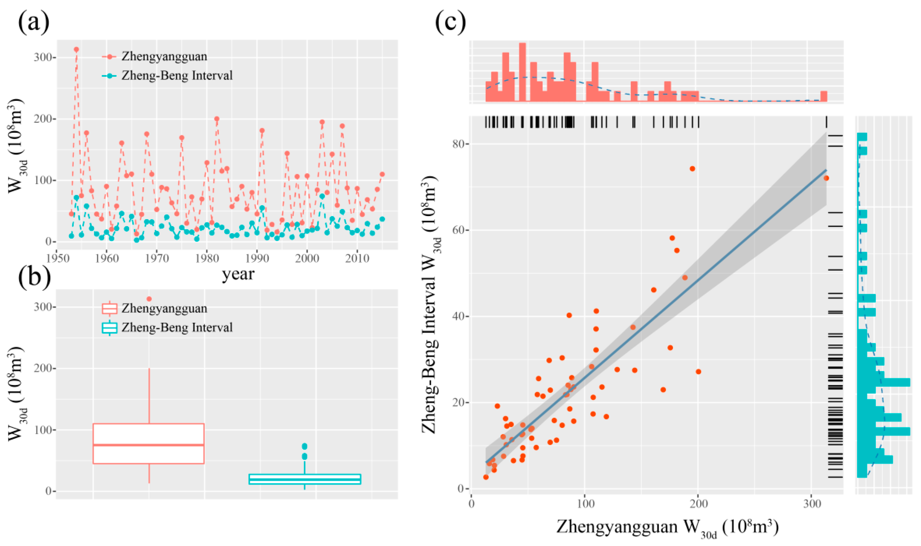
| [Min, Max] | [12.95, 313.47] | [2.72, 74.29] |
| Median | 75.27 | 19.22 |
| Mean | 85.76 | 22.51 |
| Standard deviation | 57.75 | 15.39 |
| Skewness | 1.32 | 1.45 |
| Kurtosis | 2.22 | 2.11 |
| Interquartile range | 65.04 | 15.66 |
| Region | Series | Functions | Parameters | CvM Test | RMSE | AIC | ||
|---|---|---|---|---|---|---|---|---|
| Name | Estimated Value | w2 | p | |||||
| Zhengyangguan | W30d | PE3 | [α, β, γ] | [1.921, 0.024, 4.870] | 0.027 | 0.985 | 2.881 | 668.32 |
| LN3 | [μlog, σlog, ζ] | [4.599, 0.497, −26.673] | 0.030 | 0.978 | 3.003 | 672.85 | ||
| MEV | [ξ, α, κ] | [58.042, 40.019, −0.105] | 0.034 | 0.964 | 3.013 | 674.06 | ||
| GP | [ξ, α, κ] | [16.994, 84.403, 0.227] | 0.042 | 0.924 | 3.214 | 673.34 | ||
| GAM | [β, α] | [39.100, 2.193] | 0.028 | 0.983 | 3.085 | 669.58 | ||
| GUM | [ξ, α] | [60.053, 44.544] | 0.051 | 0.869 | 3.324 | 674.90 | ||
| GLO | [ξ, α, κ] | [73.944, 28.046, −0.239] | 0.049 | 0.887 | 3.119 | 676.88 | ||
| Zheng-Beng Interval | W30d | PE3 | [α, β, γ] | [1.434, 0.077, 3.899] | 0.037 | 0.949 | 2.138 | 500.80 |
| LN3 | [μlog, σlog, ζ] | [3.064, 0.579, −2.801] | 0.024 | 0.993 | 2.084 | 489.11 | ||
| MEV | [ξ, α, κ] | [15.037, 9.770, −0.161] | 0.023 | 0.994 | 2.025 | 488.53 | ||
| GP | [ξ, α, κ] | [5.366, 19.379, 0.130] | 0.060 | 0.815 | 2.355 | 501.80 | ||
| GAM | [β, α] | [10.109, 2.227] | 0.040 | 0.936 | 2.651 | 499.99 | ||
| GUM | [ξ, α] | [15.811, 11.614] | 0.069 | 0.762 | 3.170 | 504.70 | ||
| GLO | [ξ, α, κ] | [18.972, 7.066, −0.278] | 0.028 | 0.982 | 2.369 | 503.51 | ||
| Copula Model | Parameter Name | Estimated Parameter | AIC | |
|---|---|---|---|---|
| Symmetric GH Copula | 2.7576 | −519.544 | 0.714 | |
| Two-parameter GH Copula | , | [2.1241, 0.7176] | −520.997 | 0.614 |
| Asymmetric GH Copula | , , ] | [2.7569, 1.0000, 1.0000] | −515.480 | 0.714 |
| Combination | Copula | Zhengyuangguan W30d Distribution | Zheng-Beng Interval W30d Distribution |
|---|---|---|---|
| C1 | GH2 | PE3 | PE3 |
| C2 | GH2 | PE3 | LN3 |
| C3 | GH2 | PE3 | GEV |
| C4 | GH2 | PE3 | GP |
| C5 | GH2 | PE3 | GAM |
| C6 | GH2 | PE3 | GUM |
| C7 | GH2 | PE3 | GLO |
| C8 | GH2 | LN3 | GEV |
| C9 | GH2 | GEV | GEV |
| C10 | GH2 | GP | GEV |
| C11 | GH2 | GAM | GEV |
| C12 | GH2 | GUM | GEV |
| C13 | GH2 | GLO | GEV |
| Combination | Conditional Design Regional Flood Composition Points | ||||||
|---|---|---|---|---|---|---|---|
| T = 20 | T = 50 | T = 100 | |||||
| CEC | CMLC | CEC | CMLC | CEC | CMLC | ||
| Given flood occurs at the Zhengyuanguan section | C1 | (199.22, 47.55) | (199.22, 48.98) | (244.62, 59.23) | (244.62, 62.01) | (278.18, 68.39) | (278.18, 71.76) |
| C2 | (199.22, 47.34) | (199.22, 48.37) | (244.62, 60.34) | (244.62, 61.66) | (278.18, 71.27) | (278.18, 73.34) | |
| C3 | (199.22, 47.10) | (199.22, 48.26) | (244.62, 60.83) | (244.62, 61.00) | (278.18, 72.92) | (278.18, 73.72) | |
| C4 | (199.22, 47.70) | (199.22, 50.37) | (244.62, 58.26) | (244.62, 62.14) | (278.18, 65.94) | (278.18, 70.15) | |
| C5 | (199.22, 46.50) | (199.22, 48.18) | (244.62, 56.85) | (244.62, 59.57) | (278.18, 64.83) | (278.18, 67.97) | |
| C6 | (199.22, 45.56) | (199.22, 46.91) | (244.62, 55.38) | (244.62, 57.68) | (278.18, 63.05) | (278.18, 65.81) | |
| C7 | (199.22, 46.47) | (199.22, 46.67) | (244.62, 61.34) | (244.62, 59.15) | (278.18, 75.46) | (278.18, 73.28) | |
| Given flood occurs at the Zheng-Beng interval section | C3 | (178.98, 52.27) | (181.18, 52.27) | (220.24, 68.13) | (230.76, 68.13) | (252.20, 81.69) | (264.54, 81.69) |
| C8 | (178.56, 52.27) | (180.98, 52.27) | (223.53, 68.13) | (229.34, 68.13) | (260.37 81.69) | (269.52, 81.69) | |
| C9 | (178.19, 52.27) | (179.39, 52.27) | (225.20, 68.13) | (228.18, 68.13) | (264.89, 81.69) | (271.74, 81.69) | |
| C10 | (179.48, 52.27) | (186.67, 52.27) | (213.83, 68.13) | (229.82, 68.13) | (237.23 81.69) | (253.09, 81.69) | |
| C11 | (177.86, 52.27) | (184.30, 52.27) | (217.72, 68.13) | (228.17, 68.13) | (248.45, 81.69) | (260.56, 81.69) | |
| C12 | (174.16, 52.27) | (179.31, 52.27) | (211.80, 68.13) | (220.63, 68.13) | (241.24, 81.69) | (251.81, 81.69) | |
| C13 | (176.10, 52.27) | (175.22, 52.27) | (228.12, 68.13) | (223.65, 68.13) | (276.11, 81.69) | (272.51, 81.69) | |
| T | Method | sz | S25% (1016 m3·m3) | S50% (1016 m3·m3) | S75% (1016 m3·m3) | |||
|---|---|---|---|---|---|---|---|---|
| Given flood occurs in the Zhengyangguan section | 20-year | CEC | 63 | 25.2 | 8.05 | 165 | 417 | 852 |
| 200 | 12.5 | 4.06 | 50.4 | 122 | 251 | |||
| 500 | 7.91 | 2.64 | 21.5 | 49.9 | 102 | |||
| CMLC | 63 | 25.4 (0.79%) 1 | 7.77 (−3.48%) | 162 (−1.82%) | 422 (1.20%) | 858 (0.70%) | ||
| 200 | 12.5 | 3.85 | 49.7 | 124 | 251 | |||
| 500 | 7.93 | 2.48 | 20.7 | 50.6 | 99.9 | |||
| 50-year | CEC | 63 | 32.2 | 12.4 | 397 | 957 | 1946 | |
| 200 | 17.7 | 7.05 | 130 | 313 | 631 | |||
| 500 | 11.1 | 4.45 | 51.8 | 124 | 254 | |||
| CMLC | 63 | 31.9 (−0.93%) | 11.8 (−4.83%) | 373 (−6.05%) | 891 (−6.90%) | 1866 (−4.11%) | ||
| 200 | 17.8 | 6.37 | 116 | 281 | 564 | |||
| 500 | 11.1 | 4.01 | 48.9 | 112 | 226 | |||
| 100-year | CEC | 63 | 40.1 | 18.2 | 679 | 1656 | 3369 | |
| 200 | 21.9 | 10.1 | 232 | 563 | 1146 | |||
| 500 | 13.9 | 6.41 | 94.2 | 230 | 462 | |||
| CMLC | 63 | 40 (−0.25%) | 16.7 (−8.24%) | 626 (−7.81%) | 1537 (−7.19%) | 3301 (−2.02%) | ||
| 200 | 21.6 | 8.93 | 199 | 489 | 967 | |||
| 500 | 13.9 | 5.74 | 85.2 | 201 | 409 | |||
| Given flood occurs in the Zheng-Beng interval | 20-year | CEC | 63 | 23.8 | 6.86 | 166 | 405 | 812 |
| 200 | 13.4 | 3.91 | 56.1 | 133 | 262 | |||
| 500 | 8.55 | 2.51 | 22.8 | 53.9 | 108 | |||
| CMLC | 63 | 24.6 (3.36%) | 6.95 (1.30%) | 174 (4.82%) | 410 (1.23%) | 846 (4.19%) | ||
| 200 | 13.8 | 3.94 | 55 | 137 | 275 | |||
| 500 | 8.6 | 2.51 | 21.7 | 53.1 | 109 | |||
| 50-year | CEC | 63 | 34.1 | 12.2 | 420 | 1018 | 2106 | |
| 200 | 19.3 | 7.03 | 144 | 341 | 684 | |||
| 500 | 12.1 | 4.41 | 56.9 | 137 | 280 | |||
| CMLC | 63 | 34 (−0.29%) | 12.3 (0.82%) | 405 (−3.57%) | 997 (−2.06%) | 2073 (−1.56%) | ||
| 200 | 18.4 | 6.87 | 134 | 317 | 631 | |||
| 500 | 11.6 | 4.43 | 56.6 | 129 | ||||
| 100-year | CEC | 63 | 42.2 | 18.2 | 739 | 1793 | ||
| 200 | 23.9 | 10.2 | 260 | 638 | ||||
| 500 | 14.9 | 6.41 | 102 | 253 | ||||
| CMLC | 63 | 41.9 (−0.72%) | 18.2 (0.00%) | 712 (−3.65%) | 1780 (−0.73%) | |||
| 200 | 22.6 | 10.3 | 250 | 599 | ||||
| 500 | 14.1 | 6.58 | 101 | 235 |
© 2018 by the authors. Licensee MDPI, Basel, Switzerland. This article is an open access article distributed under the terms and conditions of the Creative Commons Attribution (CC BY) license (http://creativecommons.org/licenses/by/4.0/).
Share and Cite
Mou, S.; Shi, P.; Qu, S.; Ji, X.; Zhao, L.; Feng, Y.; Chen, C.; Dong, F. Uncertainty Analysis of Two Copula-Based Conditional Regional Design Flood Composition Methods: A Case Study of Huai River, China. Water 2018, 10, 1872. https://doi.org/10.3390/w10121872
Mou S, Shi P, Qu S, Ji X, Zhao L, Feng Y, Chen C, Dong F. Uncertainty Analysis of Two Copula-Based Conditional Regional Design Flood Composition Methods: A Case Study of Huai River, China. Water. 2018; 10(12):1872. https://doi.org/10.3390/w10121872
Chicago/Turabian StyleMou, Shiyu, Peng Shi, Simin Qu, Xiaomin Ji, Lanlan Zhao, Ying Feng, Chen Chen, and Fengcheng Dong. 2018. "Uncertainty Analysis of Two Copula-Based Conditional Regional Design Flood Composition Methods: A Case Study of Huai River, China" Water 10, no. 12: 1872. https://doi.org/10.3390/w10121872