Article

Automated Laboratory Infiltrometer to Estimate Saturated Hydraulic Conductivity Using an Arduino Microcontroller Board

by
Pedro Rodríguez-Juárez
,
Hugo E. Júnez-Ferreira
*,
Julián González Trinidad
,
Manuel Zavala
,
Susana Burnes-Rudecino
and
Carlos Bautista-Capetillo
Universidad Autónoma de Zacatecas, Campus Siglo XXI, Carretera Zacatecas-Guadalajara Km. 6, Ejido La Escondida, Zacatecas 98160, Mexico
*
Author to whom correspondence should be addressed.
Water 2018, 10(12), 1867; https://doi.org/10.3390/w10121867
Submission received: 29 November 2018 / Revised: 12 December 2018 / Accepted: 14 December 2018 / Published: 17 December 2018
(This article belongs to the Special Issue Soil Hydrology for a Sustainable Land Management: Theory and Practice)

Abstract

:
This paper describes the design, calibration and testing processes of a new device named Automated Laboratory Infiltrometer (ALI). It allows to determinate in laboratory, under controlled conditions the saturated hydraulic conductivity (Ks) of altered or unaltered soil samples which is a key parameter to understand the movement of water through a porous medium. The ALI combines the advantages of three different approaches: measures vertical infiltration rates in a soil column, measures the actual volumes of vertically drained water through the soil column, and finally, uses heat as a natural tracer to determinate water flux rates through the porous medium; all those parameters are used to determinate Ks. The ALI was developed using the popular Arduino microcontroller board and commercially available sensors that give the whole system a low cost. Data from the ALI are recorded in a microSD memory so they can be easily read from any spreadsheet software helping to reduce time consuming and avoiding reading errors. The performance of this device was evaluated by comparing the water flow rates determined by the three approaches for which is designed; an excellent correlation among them was observed (worst correlation: R2 = 0.9826 and r-RSME = 0.94%).

1. Introduction

Aquifers have become an important source of water, especially in zones with low precipitation and with scarce availability of surface water. However, due to the excessive withdrawals, some aquifers have been carried out to overexploitation and their levels have been reduced drastically, e.g., in Brazil the piezometric surface has been lowered up to 100 m in some points [1], and worldwide groundwater (GW) estimated depletion is 204 ± 30 km3 y−1 [2]. This condition has several negative effects such as saline water intrusion to aquifers in coastal regions, affectations to rivers, springs and wetlands that depend on groundwater supplies, land subsidence due to pore pressure reductions [3,4] and climate changes [2]. In order to achieve an adequate planning and management of groundwater, it is necessary to improve the knowledge of its functioning; the proper understanding of groundwater flow systems is of paramount importance for hydrogeologists.
The hydraulic conductivity is a parameter used in hydrogeology to define the ease by which groundwater can flow through a porous medium [5], it is fundamental to explain the groundwater movement in the saturated zone, recharge-discharge processes in the vadose zone, transport of contaminants, etc. The hydraulic conductivity values depend on several factors such as fluid density and viscosity, packing and size of the granular material, pore connection, among others. In the vadose zone, it can take several values in time since it additionally depends on the water content and the soil water pressure head, therefore, its characterization in this zone is a difficult task due to both its spatial and temporal variability [6]. For saturated conditions, the saturated hydraulic conductivity (Ks) is applied, and due to minor changes assumed in those zones of an aquifer, values are usually kept constant through time.
Several methods to estimate Ks have been developed and they can be classified in different manners. A first approach classifies them in direct (e.g., infiltrometers, seepage meters, lysimeters, etc.) and indirect methods (use of tracers such as isotopes or heat and numerical modelling). Direct methods provide results in the short term; numerical modeling involves deep analysis of porous media physical properties. Readers can refer to Scanlon et al. [7] or Shanafield and Cook [8] for a method review and to Rosenberry and LaBaugh [9] for a detailed explanation of the most common methods. A second approach classifies them in field (e.g., pump test, slug test, single or double ring infiltrometer, Guelph permeameter) and laboratory methods (e.g., lysimeters, constant or falling head permeameter, column test).
Single ring (SRI) or double ring (DRI) infiltrometers are one of the most used devices for in-situ determination of infiltration rates and saturated hydraulic conductivity. Several studies have used infiltrometers [10,11,12,13,14]; recently, Nestingen et al. [15] made a comparison between three types of infiltrometers (modified Philip-Dunne, double-ring, and minidisk infiltrometers) and they found that the double ring infiltrometer was the most precise. With the recent advances in microelectronics, telecommunications and software, some developments have been done to automate this device [13,16,17], which has been useful to reduce time consumption and increase accuracy. Unfortunately, the infiltrometer just provides information from the surface without considering the possibility of horizontal flows. To compensate for this, some researchers have preferred to carry out infiltration tests in the laboratory under controlled conditions using test columns, so it is possible to measure not only the inflows, but also the outflows as well as others parameters such as water content, temperature, etc. [18,19].
Tracers are used in groundwater studies to determinate Ks and infiltration rates at large scales, surface water—groundwater exchanges, among others. Tracers such as coloured dye, artificial radioactive tracers [20], bromide (Br) or tritiated water (HTO) [21], potassium bromide (KBr) [22], disodium-fluorescein, sulforhodamine B or lithium [23] can be artificially injected into aquifers. However, artificial tracers represent potential environmental risks due to their high persistence in the porous medium and they require expensive equipment to measure it.
On the other hand, it has been shown that the use of heat as a tracer has certain advantages: (1) it is a natural phenomenon, therefore it does not disturb the soil or contaminate it; (2) thermal properties of soils have a narrower range of variation than their analogous hydraulic properties [24], so they can be taken directly from literature introducing small uncertainty to analysis; (3) heat measurement does not require expensive laboratory equipment; and, (4) it is more robust and less expensive than chemical tracers. Several studies have been done using temperature time series to estimate surface water-groundwater interactions [24,25,26,27,28,29,30,31]. Some other studies have been carried out in laboratory using heat as a tracer to estimate infiltration rates in test columns [18,32], see Rau et al. [33] and Halloran et al. [34] for reviews.
In this work, a new device capable to determine Ks of altered or unaltered soil samples is presented. This device named Automated Laboratory Infiltrometer (ALI) was designed to combine the characteristics and advantages of three different approaches. 1. It measures the vertical infiltration rates in a soil column; 2. It measures the real volumes of vertically drained water through the soil column, and finally, 3. It uses heat as a natural tracer to estimate water flux rates through a porous medium; these data can be used to estimate the Ks by using the Darcy equation (drained water fluxes and infiltration rates) or the Stallman equation (temperature time series). The ALI has been developed with an open source Arduino microcontroller board and commercially available sensors, which gives to the whole system a lower cost than in previous works. Details of the construction, calibration and evaluation of the ALI are described in this paper, so it can be easily reproduced at low cost by any researcher. It was tested in laboratory and statistical analyses were done to evaluate its performance.

2. Materials and Methods

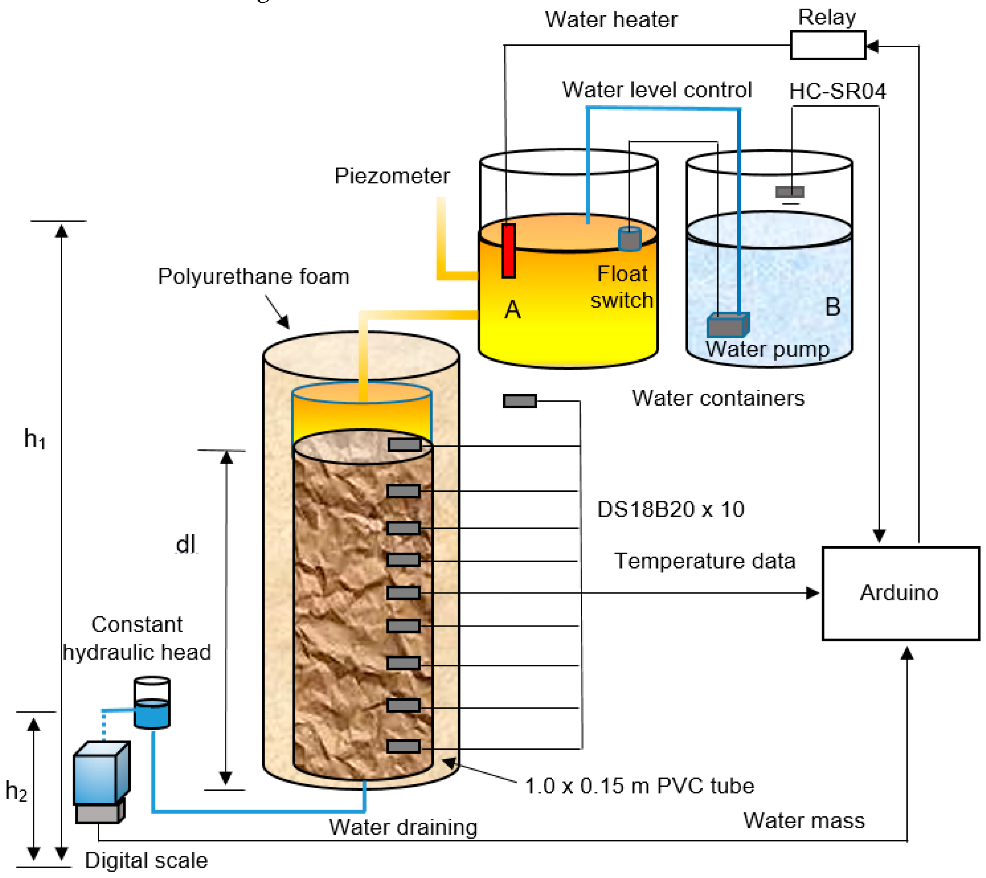
2.1. The Automated Laboratory Infiltrometer

The ALI (Figure 1) is made in a 1.0 × 0.15 m PVC tube which can be filled with any soil sample; it is wrapped with one layer of flexible polyurethane foam 1 cm thick (thermal conductivity = 0.03 Wm−1 K−1) to insulate it from the environment. Its lower end is connected to a plastic funnel and a clear hose to drain out the water; to keep the lower hydraulic head constant, the hose is connected to a small tank from the bottom and once it reaches the desired level it is drained trough the upper outlet to the container of the digital scale.
In order to estimate water flux rates through the use of temperature time series, quasi-sinusoidal heating cycles with a 6-h period are induced in the water container A using one 400 W submersible electrical heater. The heater is turned on by the Arduino for 3 h heating up the water and then switched off for 3 h, allowing the water to cool down. To measure temperature, the ALI has installed every 0.10 m along the tube, nine waterproof 1-wire digital temperature sensors DS18B20 Dallas semiconductors brand with accuracy of ±0.5 °C and 9–12 bits of resolution [35] previously calibrated (standard deviation (σ) = 0.0181 °C, coefficient of variation (cv) = 0.0626%). Additionally, one more sensor is installed outside the tube to measure the ambient temperature.
One Cytron ultrasonic ranging module HC-SR04 with resolution of 3.0 × 10⁻³ m [36] is installed on the top of the container B to measure infiltration volumes. A generic 10 kg load cell (accuracy of ±0.05% [37]) connected to an amplifier module HX711 is used to measure drained water mass.
The hydraulic head on the infiltration surface is kept quasi-constant by using a generic liquid level float switch and a submersible 6 volts water pump.
Data from all sensors are recorded in a microSD memory card and displayed on a 20 × 4 LCD. Power circuitry is handled by using a single channel relay.
A boundary condition of Dirichlet type (of constant hydraulic head) and quasi-sinusoidal periodic heating cycles were imposed at the top of the column test (water input). Water circulates downwards with free drainage at the bottom (water output) until it reaches the steady state, at this moment, a Dirichlet type boundary condition is imposed at the bottom because the water level is controlled at the container that receives the output water. The ALI can be changed to hydraulic head falling conditions just by eliminating container B and placing the HC-SR04 on container A.
The ALI has a maintenance cycle that depends of the soil under study; during this maintenance, container B is refilled, the digital scale container is emptied, and the system reestablished. This cycle can be augmented by increasing the capacity of the container B and the digital scale. Small changes on the Arduino program have to be done to increase the digital scale capacity. Container A is refilled automatically, so it does not require any maintenance during the experiment. Details of the main functions for the ALI are described below.

2.2. Data Acquisition System

The data acquisition system reads and records data from all the sensors into the microSD memory card every 5 min; these data can be easily read in any spreadsheet program such as Microsoft Excel. It controls the electrical heaters and displays the information on a 20 × 4 LCD. It is developed using the very popular and low-cost Arduino Mega 2560 microcontroller board based on the ATmega 2560 microcontroller and programmed using the open source Arduino software.

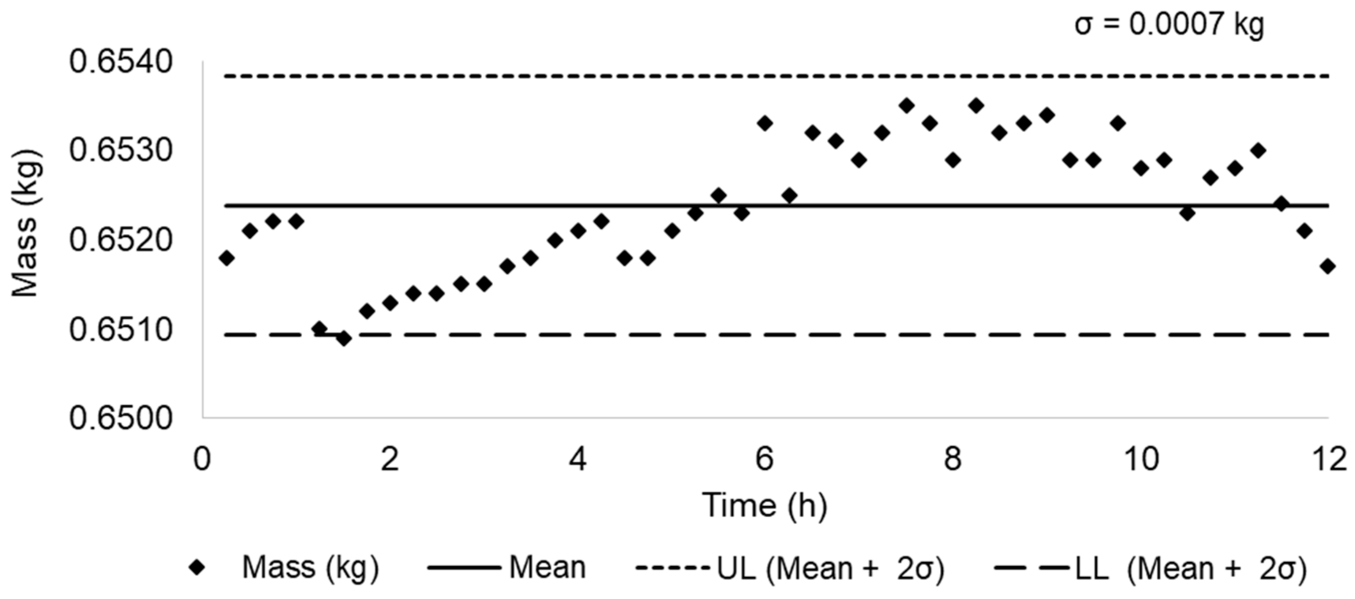
2.3. Drained Water Flux Rates Measurement

A digital scale is made by using a 10 kg load cell (a transducer capable to translate pressure into a proportional electrical signal) mounted on a wood base. Once the system is turned ON, the digital scale starts an auto-calibration subtracting the tare weight. The drained water mass is measured every 5 min and the previous value is subtracted from the new value and accumulated per hours, then it is converted to volume by V w = m w / ρ w , where V w is the volume (m3), m w is the mass (kg) and ρ w density (kg m−3) of the water. These data are used to calculate the drained water rate ( Q ) per time unit (m3 h−1). Finally, the water flux rates q (m h−1) are determined by Equation (1), where A is the cross-sectional area of the column (m2),
q = Q A
Calibration was done by applying a constant load for 12 h. Figure 2 is a control chart showing stable behavior, with σ = 7.0 × 10⁻⁴ kg and cv = 0.11%; the upper limit (UL) is the sum of 2σ and the mean; the lower limit (LL) is the result of the mean minus 2σ. A pre-processing step was done by taking 20 samples at time, then the data were filtered extracting the median, which is more robust than the mean in presence of outliers or skewed data.

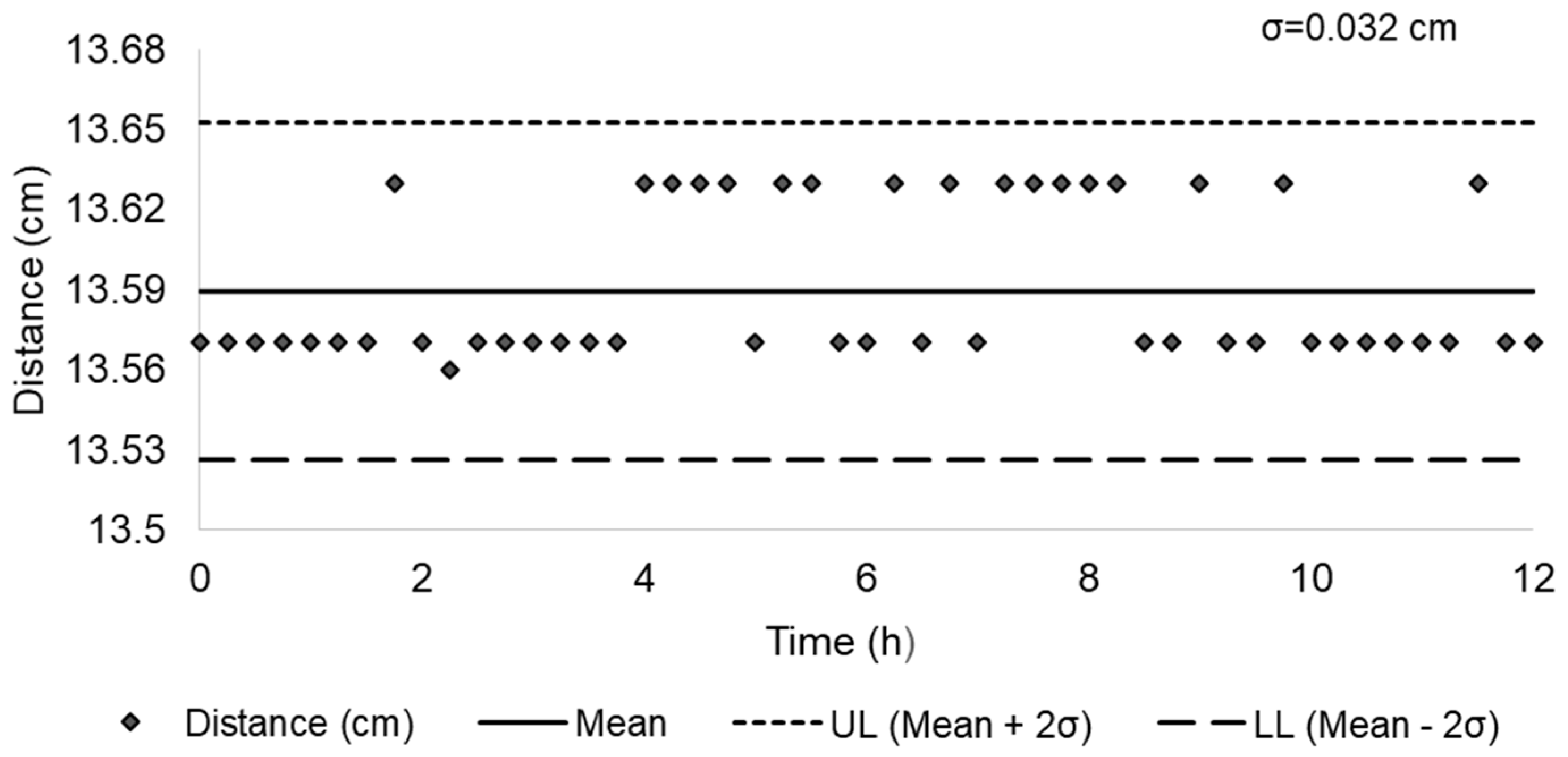
2.4. Water Flux Rates Determination by Measuring Infiltration Rates

As shown in Figure 1, there are two water containers. The container A is used to heat up the water supplied to the ALI and keep the upper hydraulic head (h1) quasi-constant. This level is maintained by the use of a float level switch with a range of 5.0 × 10⁻³ m; once the water reaches its lower level (h1-5.0 × 10⁻³ m), a water pump submerged in the container B is activated until the level reaches the upper level (h1). The infiltration rate is measured in container B by the use of an ultrasonic ranging module HC-SR04. Basically, its transmitter emits a 40 KHz ultrasonic wave when it is triggered and a timer is started. An ultrasonic pulse travels outward until it encounters an object (in this case water), the water reflects back the pulse, the ultrasonic receiver detects the reflected wave and stops the timer; this is the traveling time, which divided by two and multiplied by the sound speed, gives the distance between the sensor and the water. The increase of this distance multiplied by the cross-sectional area of the container B gives the infiltrated volume, which is accumulated per hours and considered the infiltration rate per time unit (m h−1). The water flux rates are determined by Equation (1).
The sound speeds depend on the air temperature and humidity, so, calibration was done by measuring a constant level of water for 12 h to observe the impact of the temperature and humidity daily changes. Figure 3 is a control chart showing a stable behavior through time, with σ equal to 3.0 × 10⁻⁴ m and cv equal to 0.23%; the upper limit (UL) is the sum of 2σ and the mean; the lower limit is the result of the mean minus 2σ. A pre-processing step was done by taking 20 samples at a time, then the data were filtered extracting the median.

2.5. Low Pass Filter

Data from infiltration rates, drained water flux rates and digital scale are filtered by using a moving average filter (MA). This is a low pass Finite Impulse Response (FIR) filter, used to reduce random noise, which is common on sensors and electronics devices. It is frequently used on digital signal processing and is a premier filter for time domain encoded signals [38]. The moving average filter (2) operates by averaging a number of points ( M ) from the input signal x ( ) , to produce each point in the output signal y ( ) ,
y ( i ) = 1 M j = 0 M 1 x ( i + j )

2.6. Water Flux Rates Determination by Using Temperature Time Series

2.6.1. The Heat and Fluid Transport Equation

The conduction-convection equation describes one-dimensional, anisothermal and vertical flow of an incompressible fluid through an isotropic, homogeneous porous medium,
K t δ 2 T δ z 2 q C w δ T δ z = C s δ T δ t
where K t is the thermal conductivity of the saturated porous medium (W m−1 °C−1), T is the temperature (°C), q is the infiltration flux (m s−1), C w and C s are the volumetric heat capacity of the water and soil porous media respectively (J m−3 °C−1), z is the distance along the vertical axis (m) and t is the elapsed time (s). There are some analytical solutions proposed for (3) in the scientific literature; the reader can refer to Irvine et al. [30] for a detailed review. The proposal by Hatch et al. [39] is one of the most commonly used to calculate water flux rates through porous media by using either the amplitude (4) or phase differences (5) of a periodic temperature signal between two points at different depths. This model assumes a quasi-sinusoidal temperature oscillation at the upper boundary and one directional water flow path.
q = C s C w ( 2 K e Δ z l n A r + α + v 2 2 )
| q | = α 2 ( 4 π Δ t K e P Δ z )
where
α = v 4 + ( 8 π K e P Δ z ) 2
K e = λ 0 C s + β | v f |
v f = q n e
where K e is the effective thermal diffusivity (m2 s−1), A r and Δ t are the amplitude and phase relations (dimensionless), v is the water front velocity (m s−1), P is the period of the sinusoidal signal (s), λ 0 is the baseline thermal conductivity of the saturated sediment (J s−1 m−1 °C−1), β is the thermal dispersivity (m), v f is the linear particle velocity (m s−1) and n e is the effective porosity (dimensionless). Both A r and Δ t are less influenced by errors in thermal conductivity at higher flow rates, as expected when advection becomes more important for heat transport [40]. As demonstrated by Stallman [41], analysis of diurnal temperature fluctuations may yield accurate detection of velocity to a minimum of 0.3 cm/day, so it is useful for most of the soil textures.

2.6.2. Dynamic Harmonic Regression (DHR)

Dynamic harmonic regression, developed by Young et al. [42] is a non-stationary extension of Discrete Fourier Transform (DFT), it works in both time and frequency domains, so it is useful to detect amplitude and phase variations in time. DHR is particularly useful for adaptive seasonal adjustment, signal extraction and interpolation over gaps, as well as forecasting or backcasting [42]; it is a simplification of the unobserved component model (9),
y t = T t + C t + e t
where y t is the observed time series, T t is the trend or the zero frequency component, C t is the cyclical component and e t is an irregular component assumed to be Gaussian white noise with constant variance. The cyclical component (10) is the sum of the fundamental signal and its associated harmonics
C t = i = 1 N [ a i , t cos ( ω i t ) + b i , t sin ( ω i t ) ] ,
where a i , t and b i , t are the stochastic time-varying parameters (TPV’s) and ω 1 , ω 2 , …, ω N are the fundamental frequency ( ω 1 ) and its harmonics ( ω i = i ω 1 ) up to the Nyquist frequency ( ω N ).

2.6.3. Temperature Time Series Processing

Raw data from temperature sensors are analyzed in both frequency and time domain. The analytical solution from Hatch et al. [39] uses the amplitude ratio (4) or the phase shift (5) of temperature time series to derivate seepage fluxes. So, as a first step, data are filtered by using an anti-aliasing low-pass finite impulse response (FIR) filter designed with a Kaiser window to remove high frequency noise (inherent to any electronic device) and resampled to 48 samples per fundamental cycle (day) which is recommended in order to eliminate spurious filtration artifacts. Dynamic harmonic regression (DHR) is used to isolate fundamental signals and for the extraction of phase and amplitude information. Water flux rates are determined using the analytical solutions developed by Hatch et al. [39]. Resampling, DHR, filtering process as well a water flux rate determination is done through the use of VFLUX, which is a MATLAB toolbox developed by Gordon et al. [43].
Equations (4)–(8) need certain parameters for water flux rate determination. Those parameters are soil physical and thermal properties and they can be determined either by laboratory tests or from literature as proposed by Munz et al. [44]. In this paper, thermal dispersivity and baseline thermal conductivity were taken from literature, and then they were varied until the best results of the relative root mean square error (r-RSME) were reached. Parameters of soil such as effective porosity ( n e ), volumetric heat capacity of soil ( C s ) and water ( C w ) , thermal dispersivity ( β ) and baseline thermal conductivity ( λ ) were determined experimentally in laboratory as described by Rodríguez et al. [32]. Thermal properties values were found similar to the ones reported in the literature [18,39,44], which supports the idea of a narrower variation, which is one of the advantages of the heat as a tracer. Table 1 shows the physical and thermal parameters for a sand texture soil used to estimate water flux rates with Hatch equations.

2.6.4. Soil Sample Preparation

A soil sample with sand texture according to the U.S. Department of Agriculture (USDA) soil texture classification, is previously passed through a #20 sieve (nominal sieve opening = 0.841 mm) in order to remove rocks and coarse sand before being used on the column test.

2.7. Saturated Hydraulic Conductivity

Saturated hydraulic conductivity ( K s ) is estimated by using the Darcy Equation (11) which is commonly used to calculate the Darcy velocity (one-dimensional and equivalent to the specific discharge) of water for a saturated homogeneous and isotropic porous medium,
q = K s d h d l
where q is the the Darcy velocity or the water flux rate (m s−1), K s (m s−1) is the saturated hydraulic conductivity and d h / d l is the hydraulic gradient (dimensionless); the negative sign indicates that the flow of water is in the direction of decreasing head.

3. Results

To evaluate the ALI performance, the PVC tube was filled with the altered sand texture soil sample described in the previous section. To ensure the proper soil compaction and a proper particle accommodation, water circulation through the column was maintained for 12 h with a free drainage at the bottom.

3.1. Hydraulic Boundary Conditions and Data Processing

Dirichlet boundary conditions were established as a constant hydraulic head (2.05 ± 5 × 10⁻³ m) at the top boundary and free drainage and a constant hydraulic head at the bottom boundary (0.45 m). Infiltration rates and drained rates were filtered by using a low pass filter; water flux rates were determined and fitted using a MATLAB polynomial fitting.

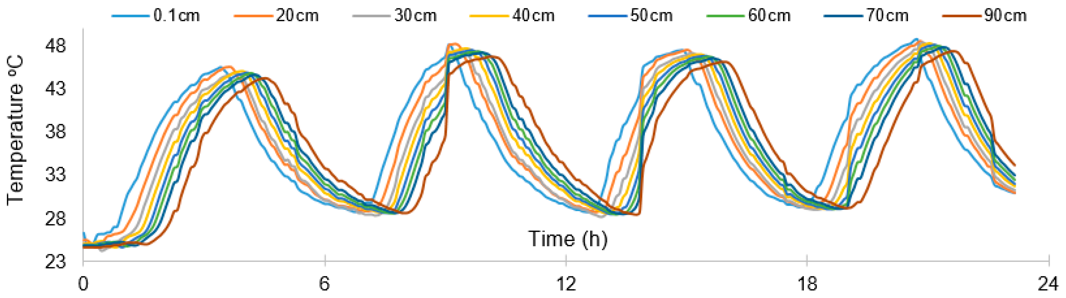
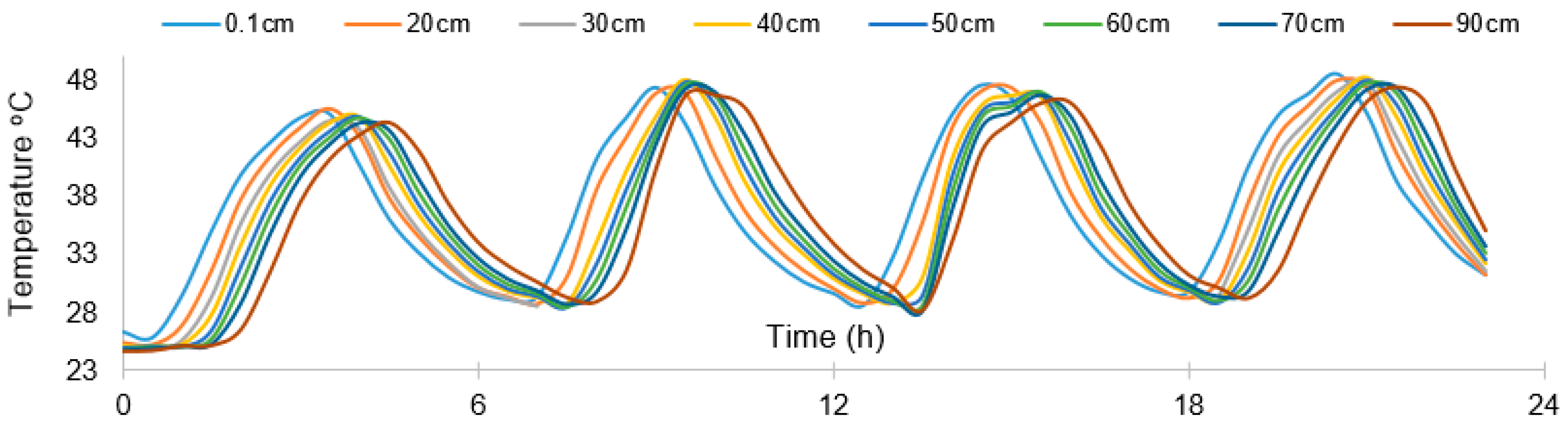
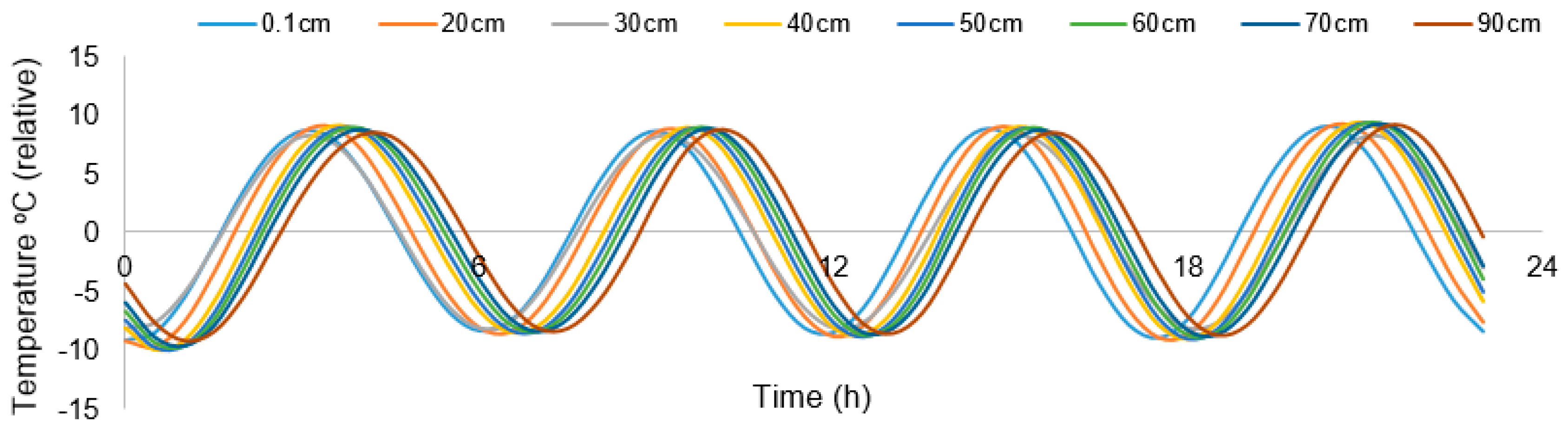
3.2. Temperature Boundary Conditions and Data Processing

Six hours quasi-sinusoidal heating cycles with an amplitude of 10 °C were induced in container A. Six-hour cycles (cyclical component) were chosen to easily distinguish from the daily temperature cycle (trend).
Temperature data were sampled every five minutes for all the sensors. Figure 4 shows raw temperature signal from eight sensors indicating the depth at which they were installed along the vertical axis. The artificially induced 6-h cycles are easily observable as well as the long-term trend; the signal looks noisy, amplitude ratio is not easy to distinguish due to the proximity of the sensors but phase delays ( Δ t ) are more visible, especially between the points 0.1 cm and 90 cm, which is more distinguishable. Raw temperature data were resampled to 48 samples per fundamental cycle (24 h); this was done to reduce noise. Figure 5 shows temperature signals after being resampled; it can be seen that the noise has been reduced but some still remains, especially on the crests and troughs. Figure 6 shows the temperature signals after filtering and trend removal; now the signal appears without noise, relative temperature changes are clearly observable as well as the phase delays ( Δ t ). Because amplitude ratio between signals is small, water flux rates calculations were done using only (5) and fitted using a MATLAB polynomial fitting.

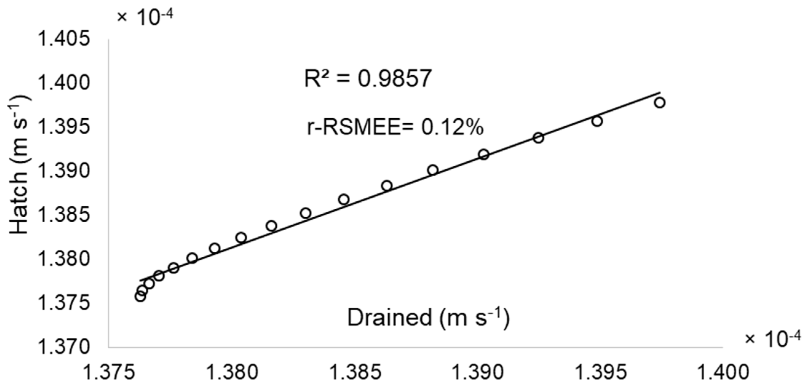
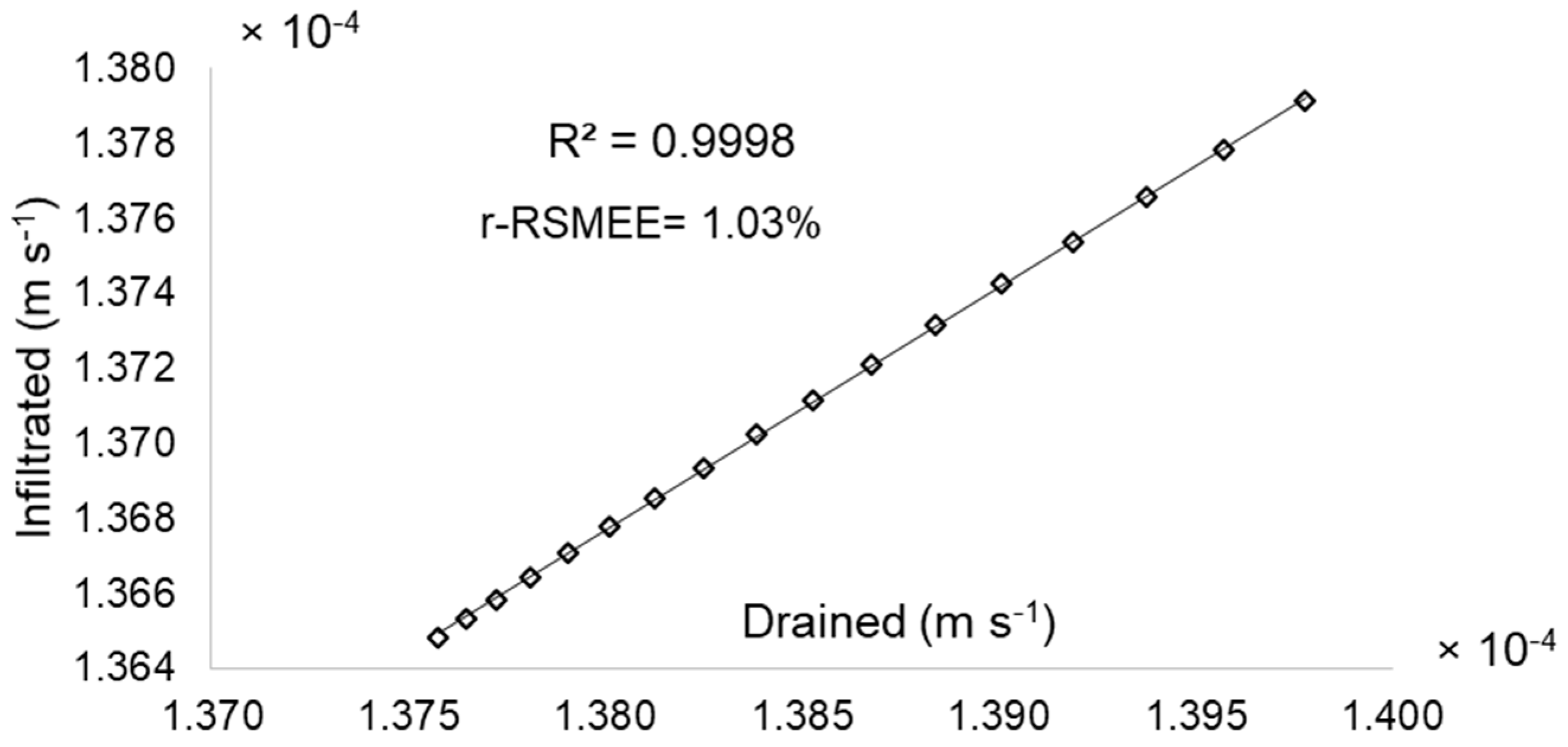
3.3. Water Flux Rates Comparison

Figure 7 shows the water flux rates ( q ) determined by the three different approaches under saturated conditions: Infiltrated (determined by measuring the infiltration rates), Drained (determined by measuring the drained water) and Hatch (calculated by VFLUX). As it can be seen, there is a clear trend for all the curves; they start with higher q values and finally they tend to stabilize (after 15 h) once the soil gets almost fully saturated (trapped air bubbles prevent full saturation). Stabilization time depends on different factors such as physical properties and initial boundary conditions of the porous media. Initially, Infiltrated water flux rates are bigger than Drained because it takes more time for the water reaching the lower end and the steady state flow condition. On the other hand, the analytical solution from Hatch et al. [39] was developed for saturated conditions, so Hatch water flux rates must be considered once the steady state is reached. As Figure 7 shows, the three water flux rates look very similar after stabilization.
Correlations between the results of the three different approaches were determined after the steady state was reached. Figure 8 shows the correlation between the results obtained by Hatch and Drained. Figure 9 shows the correlation between the results obtained by Hatch and Infiltrated; and Figure 10 shows the correlation between Drained and Infiltrated. Values of the coefficient of determination (R2) and relative root mean square error (r-RSME) are also shown.
As described by Loutfi et al. [45], R2 expresses the correlation between the measured values and the estimated ones; the best approximation corresponds to the highest R2 (closer to 1), RMSE shows the difference between the measured values and the predicted ones; it indicates the scattering of data around a straight line inclined 45°. The approximation is better if RMSE is minimal (tends to 0). Normalized root means square error (nRSME) or relative root mean square error (r-RSME) is calculated by dividing RMSE with the average value of measured data. According to Despotovic et al. [46], model accuracy is considered excellent when r-RMSE is less than 10%, good if 10% < r-RMSE < 20%, fair if 20% < r-RMSE < 30%, and poor if r-RMSE > 30%. Therefore, an excellent correlation among the methods was found, which indicates that the developed device (ALI) is able to estimate efficiently water flux rates by three different methods, giving more confidence in its results.

3.4. Determination of Saturated Hydraulic Conductivity

Saturated hydraulic conductivity Ks was determined by using (11), considering h1 = 2.05 m, h2 = 0.45 m, dl = 1.0 m and the water flux rates in steady state conditions from each of the three approaches. On average, the saturated hydraulic conductivity was 8.61 × 10⁻⁵ m s−1, which is within the range of the values reported on the saturated hydraulic conductivity in relation to the soil texture table from the U.S. Department of Agriculture (USDA) [47] which gives a range of 4.2 × 10⁻⁵ to 1.41 × 10⁻⁴ m s−1 for soils with sand textures. Table 2 shows the average Ks from the three approaches.

4. Conclusions

The saturated hydraulic conductivity is a key parameter to understand the groundwater movement, natural and artificial recharge-discharge of aquifers as well as others hydrological processes such as contaminant transport, among others. There are several methods and devices used to determine Ks for a porous medium; in this paper, a new device and the methodology needed to calculate Ks by three different approaches simultaneously is presented.
A new Automated Laboratory Infiltrometer (ALI) is developed by using a very popular Arduino Mega 2560 Microcontroller board and commercially available sensors; giving the total system a cost of around 200.00 USD, which is very low compared to a single commercial grade sensor. Furthermore, the ALI provides temperature time series, infiltration rates and drained water volumes which allow researchers to calculate water flux rates in altered or unaltered soil samples by three different approaches: one indirect by using heat as a tracer (Stallman equation) and two direct methods, i.e., vertical infiltration rates and drained water volumes (Darcy).
Drained water volumes provided by the ALI are used to verify that the steady state flow is reached; it is approximately the time where the curves for the three approaches used to calculate the water flux rates coincide, therefore, the most trustable value for Ks is determined from this point onwards. Furthermore, temperature time series could be used to determine hydraulic conductivity in unsaturated conditions without using water content sensors or tensiometers which are more expensive in comparison with temperature sensors.
Thermal properties of soils determined by the ALI in laboratory can be used as an alternative way to determine Ks in the field and to measure water interaction (upwards and downwards flows) in the vadose zone in a continuous manner. Long-term temperature data are easier and cheaper to take than the commonly used tracers that require more specialized equipment and knowledge.
The ALI was tested and excellent correlations between the three approaches used to determinate Ks were obtained (R2 = 0.9826 and r-RSME = 0.94% between Infiltrated and Hatch; R2 = 0.9857 and r-RSME = 0.12% among Hatch and Drained; and R2 = 0.9826 and r-RSME = 0.94% between Infiltrated and Drained). The saturated hydraulic conductivity determined for the three methods falls inside the ranges established by the USDA for the analyzed soil, which proved its efficiency.
Analytical solutions from Hatch et al., the Darcy equation as well as the infiltrometer, are very useful to measure water flux rates and hydraulic conductivity in saturated conditions. However, in order to obtain a better picture of the whole infiltration process (unsaturated and saturated conditions) some improvements can be done to the ALI, such as the incorporation of water content sensors and electronic tensiometers. Those additional devices will provide more parameters, allowing researchers to use, for instance, the Richards equations for estimating hydraulic conductivity values for unsaturated conditions.

Author Contributions

Conceptualization, Methodology and Writing-Original Draft Preparation, P.R.-J.; Supervision, Writing—Review & Editing, H.E.J.-F.; Investigation and Resources, M.Z. and J.G.T.; Software, S.B.-R.; Project Administration, C.B.-C.

Funding

This research received no external funding.

Acknowledgments

First author would like to acknowledge the Mexican National Council for Science and Technology (CONACYT) for the scholarship awarded for doctoral studies in engineering sciences.

Conflicts of Interest

The authors declare no conflict of interest.

References

  1. De Luna, R.M.R.; Garnés, S.J.D.A.; Cabral, J.J.D.S.P.; dos Santos, S.M. Groundwater overexploitation and soil subsidence monitoring on Recife plain (Brazil). Nat. Hazards 2017, 86, 1363–1376. [Google Scholar] [CrossRef]
  2. Taylor, R.G. Ground water and climate change. Nat. Clim. Chang. 2012, 3, 322–329. [Google Scholar] [CrossRef] [Green Version]
  3. Custodio, E. Aquifer overexploitation: What does it mean? Hydrogeol. J. 2002, 10, 254–277. [Google Scholar] [CrossRef]
  4. Fetter, C.; Boving, T.; Kreamer, D. Contaminant Hydrogeology; Waveland Press Inc.: Long Grove, IL, USA, 2017; ISBN 978-14786-3279-5. [Google Scholar]
  5. Tang, Y.; Zhou, J.; Yang, P.; Yan, J.; Zhou, N. Groundwater Engineering; Tongji University Press/Springer: Shanghai, China, 2016; ISBN 978-981-10-0669-2. [Google Scholar]
  6. Mertens, J.; Madsen, H.; Feyen, L.; Jacques, D.; Feyen, J. Including prior information in the estimation of effective soil parameters in unsaturated zone modelling. J. Hydrol. 2004, 294, 251–269. [Google Scholar] [CrossRef]
  7. Scanlon, B.R.; Healy, R.W.; Cook, P.G. Choosing appropriate techniques for quantifying groundwater recharge. Hydrogeol. J. 2002, 10, 18–39. [Google Scholar] [CrossRef]
  8. Shanafield, M.; Cook, P.G. Transmission losses, infiltration and groundwater recharge through ephemeral and intermittent streambeds: A review of applied methods. J. Hydrol. 2014, 511, 518–529. [Google Scholar] [CrossRef]
  9. Rosenberry, D.O.; LaBa ugh, J.W. Field Techniques for Estimating Water Fluxes between Surface Water and Ground Water; USGS: Reston, VA, USA, 2008. Available online: https://pubs.usgs.gov/tm/04d02/ (accessed on 7 December 2018).
  10. Xu, X.; Lewis, C.; Liu, W.; Albertson, J.D.; Kiely, G. Analysis of single-ring infiltrometer data for soil hydraulic properties estimation: Comparison of BEST and Wu methods. Agric. Water Manag. 2012, 107, 34–41. [Google Scholar] [CrossRef]
  11. Lai, J.; Luo, Y.; Ren, L. Numerical evaluation of depth effects of double-ring infiltrometers on soil saturated hydraulic conductivity measurements. Soil Sci. Soc. Am. J. 2011, 76, 867–875. [Google Scholar] [CrossRef]
  12. Kadam, A.S. Determination of infiltration rate for rite selection of artificial water recharge: An experimental study. Int. J. Sci. Res. 2016, 5, 699–705. [Google Scholar] [CrossRef]
  13. Fatehnia, M.; Paran, S.; Kish, S.; Tawfiq, K. Automating double ring infiltrometer with an Arduino microcontroller. Geoderma 2016, 262, 133–139. [Google Scholar] [CrossRef]
  14. Vand, A.S.; Sihag, P.; Singh, B.; Zand, M. Comparative evaluation of infiltration models. KSCE J. Civ. Eng. 2018, 22, 4173–4184. [Google Scholar] [CrossRef]
  15. Nestingen, R.; Asleson, B.C.; Gulliver, J.S.; Hozalski, R.M.; Nieber, J.L. Laboratory Comparison of Field Infiltrometers. J. Sustain. Water Built Environ. 2018, 4. [Google Scholar] [CrossRef]
  16. Arriaga, F.J.; Kornecki, T.S.K.; Balkcom, K.S.B.; Raper, R.L. A method for automating data collection from a double-ring infiltrometer under falling head conditions. Soil Use Manag. 2010, 26, 61–67. [Google Scholar] [CrossRef]
  17. Di Prima, S.; Lassabatere, L.; Bagarello, V.; Iovino, M.; Angulo-Jaramillo, R. Testing a new automated single ring infiltrometer for Beerkan infiltration experiments. Geoderma 2015, 262, 20–34. [Google Scholar] [CrossRef]
  18. Lautz, L.K. Observing temporal patterns of vertical flux through streambed sediments using time-series analysis of temperature records. J. Hydrol. 2012, 464–465, 199–215. [Google Scholar] [CrossRef]
  19. Salas-García, J.; Garfias, J.; Martel, R.; Bibiano-Cruz, L. A low-cost automated test column to estimate soil hydraulic characteristics in unsaturated porous media. Geofluids 2017, 2017, 6942736. [Google Scholar] [CrossRef]
  20. IAEA. Use of Artificial Tracers in Hydrology IAEA-TECDOC-601; International Atomic Energy Agency: Vienna, Austria, 1991; ISSN 1011-4289. [Google Scholar]
  21. Yeh, Y.; Lee, C.; Chen, S. A tracer method to determinate hydraulic conductivity and effective porosity of saturated clays under low gradients. Groundwater 2000, 38, 522–529. [Google Scholar] [CrossRef]
  22. Hwang, H.; Jeen, S.; Suleiman, A.A.; Lee, K. Comparison of saturated hydraulic conductivity estimated by three different methods. Water 2017, 9, 942. [Google Scholar] [CrossRef]
  23. Mosthaf, K.; Brauns, B.; Fjordbøge, A.S.; Rohde, M.M.; Kerrn-Jespersen, H.; Bjerg, P.L.; Binning, P.J.; Broholm, M.M. Conceptualization of flow and transport in a limestone aquifer by multiple dedicated hydraulic and tracer tests. J. Hydrol. 2018, 561, 532–546. [Google Scholar] [CrossRef]
  24. Stonestrom, D.A.; Constantz, J. Heat as a Tool for Studying the Movement of Ground Water near Streams; USGS Circular 1260; USGS: Reston, VA, USA, 2003. Available online: https://pubs.usgs.gov/circ/2003/circ1260/pdf/Circ1260.pdf (accessed on 12 July 2018).
  25. Ronan, A.D.; Prudic, D.E.; Thodal, C.E.; Constantz, J. Field study and simulation of diurnal temperature effects on infiltration and variably saturated flow beneath an ephemeral stream. Water Resour. Res. 1998, 34, 2137–2153. [Google Scholar] [CrossRef] [Green Version]
  26. Thomas, C.L.; Steward, A.E.; Constantz, J.E. Determination of Infiltration and Percolation Rates along a Reach of the Santa Fe River near La Bajada New Mexico; U.S. Geological Survey, Water-Resources Investigations Report 00-4141; USGS: Reston, VA, USA, 2000. [CrossRef]
  27. Arriaga, M.A.; Leap, D.I. Using solver to determine vertical groundwater velocities by temperature variations. Hydrogeol. J. 2006, 14, 253–263. [Google Scholar] [CrossRef]
  28. Birkel, C.; Soulsby, C.; Irvine, D.I.; Malcolm, I.; Lautz, L.K.; Tetzlaff, D. Heat-based hyporheic flux calculations in heterogeneous salmon spawning gravels. Aquat. Sci. 2016, 78, 203–213. [Google Scholar] [CrossRef]
  29. Kurylyk, B.L.; Irvine, D.J.; Carey, S.K.; Briggs, M.A. Heat as a groundwater tracer in shallow and deep heterogeneous media: Analytical solution, spreadsheet tool, and field applications. Hydrol. Process. 2017, 31, 2648–2661. [Google Scholar] [CrossRef] [PubMed]
  30. Irvine, D.J.; Briggs, M.A.; Lautz, L.K.; Gordon, R.P.; McKenzie, J.M.; Cartwright, I. Using Diurnal Temperature Signals to Infer Vertical Groundwater-Surface Water Exchange. Groundwater 2016, 55, 10–26. [Google Scholar] [CrossRef] [PubMed]
  31. Rodríguez-Rodríguez, M.; Fernández-Ayuso, A.; Hayashi, M.; Moral-Martos, F. Using water temperature, electrical conductivity, and pH to Characterize surface–groundwater relations in a shallow ponds system (Doñana National Park, SW Spain). Water 2018, 10, 1406. [Google Scholar] [CrossRef]
  32. Rodríguez, P.; Júnez-Ferreira, H.E.; González, J.; de la Rosa, J.I.; Galván, C.; Burnes, S. Vadose zone hydraulic conductivity monitoring by using an Arduino data acquisition system. In Proceedings of the 2018 International Conference on Electronics, Communications and Computers, Cholula, Mexico, 21–23 February 2018; pp. 80–85. [Google Scholar] [CrossRef]
  33. Rau, G.C.; Andersen, M.S.; McCallum, A.M.; Roshan, H.; Acworth, R.I. Heat as a tracer to quantify water flow in near-surface sediments. Earth Sci. Rev. 2014, 10, 41–58. [Google Scholar] [CrossRef]
  34. Halloran, L.J.; Rau, G.C.; Andersen, M.S. Heat as a tracer to quantify processes and properties in the vadose zone: A review. Earth Sci. Rev. 2016, 159, 358–373. [Google Scholar] [CrossRef]
  35. Programmable Resolution 1-Wire Digital Thermometer. Available online: https://datasheets.maximintegrated.com/en/ds/DS18B20.pdf (accessed on 12 July 2018).
  36. Product Users Manual HC-SR04 Ultrasonic Sensor. Available online: https://docs.google.com/document/d/1Y-yZnNhMYy7rwhAgyL_pfa39RsB-x2qR4vP8saG73rE/edit (accessed on 12 July 2018).
  37. Micro Load Cell Datasheet. Available online: https://www.robotshop.com/media/files/pdf/datasheet-3133.pdf (accessed on 12 July 2018).
  38. Smith, S.W. The Scientist and Engineer’s Guide to Digital Signal Processing. DSP Guide 1997, 423–450. Available online: http://www.dspguide.com/pdfbook.htm (accessed on 12 July 2018). [CrossRef]
  39. Hatch, C.E.; Fisher, A.T.; Revenaugh, J.S.; Constantz, J.; Ruehl, C. Quantifying surface water-groundwater interactions using time series analysis of streambed thermal records: Method development. Water Resour. Res. 2006, 42. [Google Scholar] [CrossRef] [Green Version]
  40. Shanafield, M.; Hatch, C.; Pohll, G. Uncertainty in thermal time series analysis estimates of streambed water flux. Water Resour. Res. 2011, 47. [Google Scholar] [CrossRef] [Green Version]
  41. Stallman, R.W. Steady One-Dimensional Fluid Flow in a Semi-Infinite Porous Medium with Sinusoidal Surface Temperature. J. Geophys. Res. 1965, 70, 2821–2827. [Google Scholar] [CrossRef]
  42. Young, P.; Pedregal, D.; Tych, W. Dynamic harmonic regression. J. Forecast. 1999, 18, 369–394. [Google Scholar] [CrossRef] [Green Version]
  43. Gordon, R.P.; Lautz, L.K.; Briggs, M.A.; McKenzie, J.M. Automated calculation of vertical pore-water flux from field temperature time series using the VFLUX method and computer program. J. Hydrol. 2012, 420–421, 142–158. [Google Scholar] [CrossRef]
  44. Munz, M.; Oswald, S.E.; Schmidt, C. Sand box experiments to evaluate the influence of subsurface temperature probe design on temperature based water flux calculation. Hydrol. Earth Syst. Sci. 2011, 15, 3495–3510. [Google Scholar] [CrossRef] [Green Version]
  45. Loutfi, H.; Bernatchou, A.; Raoui, Y.; Tadili, R. Learning Processes to Predict the Hourly Global, Direct, and Diffuse Solar Irradiance from Daily Global Radiation with Artificial Neural Networks. Int. J. Photoenergy 2017, 2017, 4025283. [Google Scholar] [CrossRef]
  46. Despotovic, M.; Nedic, V.; Despotovic, D.; Cvetanovic, S. Evaluation of empirical models for predicting monthly mean horizontal diffuse solar radiation. Renew. Sustain. Energy Rev. 2016, 56, 246–260. [Google Scholar] [CrossRef]
  47. Saturated Hydraulic Conductivity in Relation to Soil Texture. Available online: https://www.nrcs.usda.gov/wps/portal/nrcs/detail/soils/survey/office/ssr10/tr/?cid=nrcs144p2_074846 (accessed on 12 July 2018).
Figure 1. The Automated Laboratory Infiltrometer.
Water 10 01867 g001
Figure 2. Digital scale calibration along 12 h by applying a constant load.
Water 10 01867 g002
Figure 3. Ultrasonic ranging module calibration along 12 h.
Water 10 01867 g003
Figure 4. Raw temperature time series from eight sensors installed at different depths and sampled every 5 min.
Water 10 01867 g004
Figure 5. Resampled temperature time series from eight sensors, sampling rate was reduced to 48 samples per fundamental cycle. There is still some noise on the crests and troughs. Phase delays can be observed, amplitude ratios are not so observable due to the proximity between the temperature sensors.
Water 10 01867 g005
Figure 6. Resampled and filtered temperature time series. A low-pass FIR filter was used to remove high-frequency noise and Dynamic Harmonic Regression (DHR) to remove the long-term trend. Only the changes in amplitude due to artificially induced heating cycles remain.
Water 10 01867 g006
Figure 7. Comparison of water flux rates determined by three approaches. There is a trend to start with higher q values and then the curves tend to stabilize. A high similarity among the curves can be observed once the steady state has been reached.
Water 10 01867 g007
Figure 8. Correlation between Hatch water flux rates and Drained water flux rates.
Water 10 01867 g008
Figure 9. Correlation between Infiltrated water flux rates and Hatch water flux rates.
Water 10 01867 g009
Figure 10. Correlation between Infiltrated water flux rates and Drained water flux rates.
Water 10 01867 g010
Table 1. Physical and thermal parameters of the soil and water used for water flux rates calculation by using analytical solution for heat and transport Equation (3).
ParametersDeterminedUnits
Effective porosity ( n e )0.28dimensionless
Volumetric heat capacity of soil ( C s )0.5Cal cm−3 °C−1
Volumetric heat capacity of water ( C w )1.0Cal cm−3 °C−1
Thermal dispersivity ( β )0.001M
Baseline thermal conductivity ( λ 0 )0.0045Cal s−1 cm−1 °C−1
Table 2. Average saturated hydraulic conductivity determined for the three approaches and range of values reported by the U.S. Department of Agriculture (USDA) for sand texture soils.
ApproachKsUnits
Heat as a tracer a8.6318 × 10−5m s−1
Infiltrated b 8.6384 × 10⁻⁵m s−1
Drained c8.5680 × 10−5m s−1
USDA d4.2 × 10−5 to 1.41 × 10⁻⁴m s−1
a Ks determined using heat as tracer and the analytical solution from Hatch et al. [39]. b Ks determined by measuring infiltration rates from the top. c Ks determined by measuring drained flux rates from the bottom. d Ranges of values of Ks for soils with sand texture reported by the USDA [47].

