Flow Analysis through Collector Well Laterals: A Case Study from Sonoma County Water Agency, California

Abstract

The Sonoma County Water Agency (SWCA) uses six radial collector wells along the Russian River west of Santa Rosa, to provide water for several municipalities and water districts in north-western California. Three collector wells (1, 2, and 6) are located in the Wohler area, and three collector wells (3, 4, and 5) are located in the Mirabel area. The objective of this paper is to highlight the performance of the three collector wells located in the Mirabel area since their construction. The 2015 investigation showed a lower performance of Collectors 3 and 4 compared to their original performances after construction in 1975, while the performance of Collector 5 was relatively stable since 1982. The potential change in capacity could be due to the increase in encrustation observed during the visual inspection of laterals in all three collector wells. Overall, the three collectors are still within the optimal design parameters (screen entrance velocity < 0.305 m min⁻¹ and axial flow velocity of lateral screens < 1.524 m s⁻¹).

1. Introduction

Several municipalities (i.e., the cities of Santa Rosa, Sonoma, Cotati, Rohnert Park, and Petaluma) and water districts (i.e., the Forestville Water District, Valley of the Moon Water District, North Marin Water District, and Marin Municipal Water District) in Sonoma and Marin Counties receive water from the Sonoma County Water Agency (SWCA). The SCWA water system has an estimated peak production capacity of 4.907 m³ s⁻¹. The SWCA uses six radial collector wells, along the Russian River west of Santa Rosa, to provide water for approximately 570,000 people [1]. Three collector wells (1, 2, and 6) are located in the Wohler area, and three collector wells (3, 4, and 5) are located in the Mirabel area [1].

In 1998, a preliminary investigation highlighted declined capacities (−24 to −77%) of the collector wells compared to their original capacities. The declines were more pronounced in the oldest collector wells (e.g., collector wells 1 and 2) [2]. Clogging of lateral well screens, clogging of the aquifer adjacent to the lateral well screens, compaction of the alluvial aquifer material due to long-term pumping, problems with pumping equipment in the collectors, decreased recharge from the ponds and/or river due to long-term silt/organic material build-up or changes in the operation of the inflatable dam, and regional declines in groundwater levels due to changes in precipitation, river discharge, and/or groundwater extraction were among the possible reasons [1]. However, data evaluation was highly impacted by the operations of nearby collectors during the testing.

To have a better understanding of the status (i.e., magnitude, rate, and causes of the loss of capacity) of each collector well, SCWA developed a program to evaluate flow to the collector wells in fixed time intervals (about five years). The collector wells located in the Mirabel area were investigated in 2010 and 2015 [1,3], while the collector wells in the Wohler area were investigated in 2010 and will be investigated in 2018–2019.

The objective of this paper is to show the performance of three collector wells (3, 4, and 5) located in the Mirabel area since their construction. Additionally, we also show the flow variations along the laterals (along the length and among themselves). We also compare the design parameters such as theoretical screen entrance velocity and axial flow velocity for the lateral screens as well as comparing fluxes through individual laterals. The study is unique in the sense that it attempts to examine flow variation through lateral screens.

2. Materials and Methods

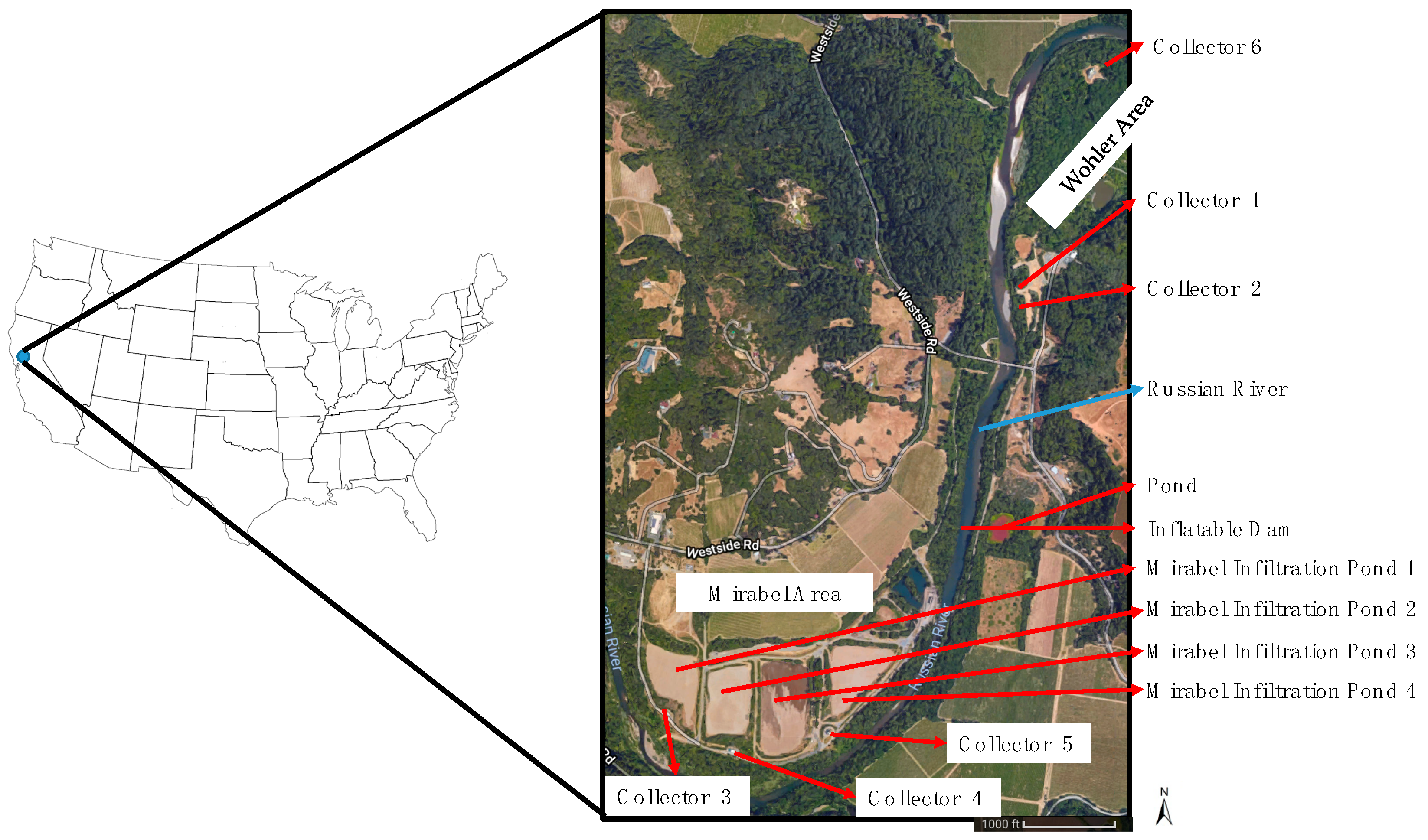
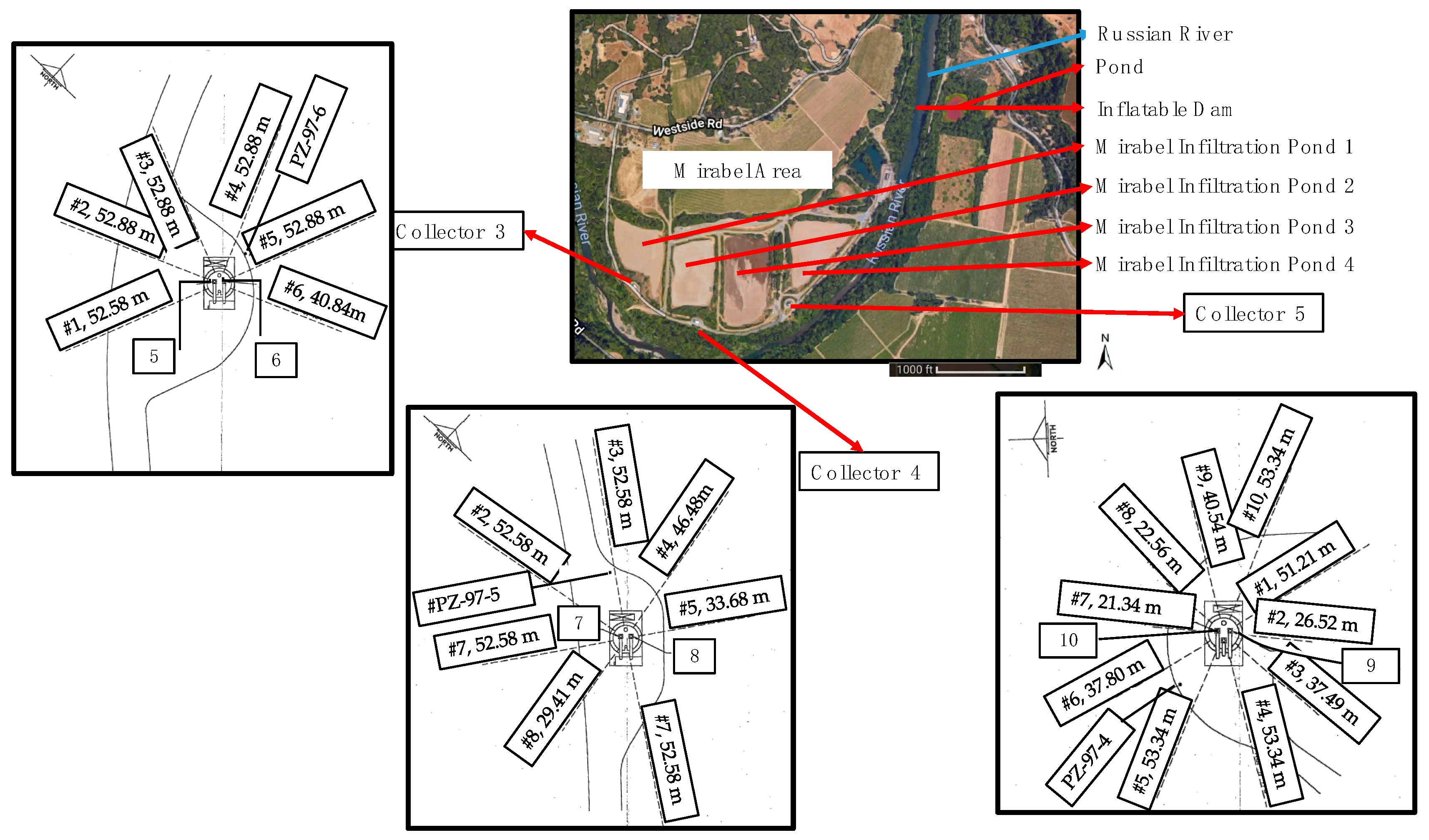
2.1. Description of the Riverbank Filtration (RBF) Sites

The Mirabel area is located approximately one mile south of the west bank of the Russian River (Figure 1). The wells extract water from the unconsolidated alluvial aquifer adjacent to and beneath the Russian River using large-volume Ranney-type (lateral) collector wells. The pumping wells induce large vertical fluxes from the river and nearby the infiltration ponds [4]. An inflatable dam and four infiltration ponds are present in this area (Figure 1).

To account for the low flow periods, May to November, SCWA raises the inflatable dam which creates a low-velocity pool of water that extends approximately 2.5 km upstream and raises the stage of the river. A higher river stage produces a pressure gradient that forces water into the streambed and recharges the alluvial aquifer. The dam also diverts water to infiltration ponds that flank the river and water quickly enters the underlying aquifer [5]. Collector wells 3 and 4 were constructed in 1975, while collector well 5 was constructed in 1982 (Table S1). The three collector wells consist of 3.96 m inside diameter steel-reinforced concrete caissons. Collector wells 3, 4, and 5 have 6, 8, and 10 laterals (25.4-cm diameter mild steel), respectively (Table S1). Laterals range between 21.34 and 53.34 m (Table S2). Additional details are included in Tables S1 and S2 (Figure 2) [1,3].

The alluvium along the Russian River is the primary source of water production for SCWA. The Russian River is approximately 180 km long, originating from the Laughlin Range of California and draining to the Pacific Ocean near Jenner, California. The river drains a basin of 3866 km². The west coast of California receives most of its precipitation in the winter months. The US Geological Survey gage at Guerneville, California (CA) indicates a long-term mean flow of about 64 m³ s⁻¹ with a maximum exceeding 2888 m³ s⁻¹ during peak flow events. The minimum flow recorded at the gage is 0.02 m³ s⁻¹ [6]. As the Russian River is home to certain species of salmonid fish that migrate upstream for spawning, SCWA has installed fish ladders around the inflatable rubber dam for ease of fish migration. The ponded water behind the dam as well as in the recharge ponds encourages weed and algae growth during summer and also allows fine particles to settle to the bottom. This is also speculated to be one of the reasons for decreasing recharge capacity of the riverbed as well as the recharge ponds. The river is underlain primarily by alluvium and river channel deposits consisting of unconsolidated sands and gravels, with thin layers of silt and sand [7]. In the investigated area, the alluvial aquifer is bounded by metamorphic bedrock and is considered impermeable relative to the alluvial materials [7]. The shallow aquifer sediments in the investigated site have a measured hydraulic conductivity between 5.5 × 10⁻⁵ to 2.0 × 10⁻⁴ m s⁻¹ and from 1.4 × 10⁻⁵ to 2.6 × 10⁻⁴ m s⁻¹ within the same area using seepage meter methods [5,7].

2.2. Evaluation Procedures

One week prior to the initiation of the constant rate test pumping, the collector wells were shut off to allow for recovery of the water table. Pressure transducers equipped with data loggers (In-Situ Inc., Fort Collins, CO, USA) were installed before shutting down. The bottom floor and interior walls of the caisson, pump intakes, gate valves, and stem riser assemblies, if present, were visually inspected by a diver in October/November 2010 and October 2015 for collector wells 3, 4, and 5 [1,3]. Before diving in each of the collector well caissons for inspection and testing, chlorination of the collector water was temporarily ceased as a health and safety consideration.

The wall thickness of each of the lateral screens was estimated using an underwater ultrasonic digital thickness gauge (Cygnus Instrument Inc. Annapolis, MD, USA). The gauge (accuracy: ±0.05 mm) was inserted into the section of the lateral nearest the caisson and thickness measurements were obtained at 0°, 90°, 180°, and 270° from the vertical position for the three collector wells. To evaluate capacity, the collector wells were separately pumped continuously for approximately five days. During the constant rate capacity test, the collector well undergoing testing was placed back on-line at a controlled pumping rate roughly comparable to typical operating conditions [1,3].

Periodically, water levels within the collector well and five site monitoring wells were measured using an electric tape (accuracy: ±0.3 cm). Measurement of pH (accuracy: ±0.2), oxygen reduction potential, redox potential (ORP), (accuracy: ±20 mV), dissolved oxygen, DO, (accuracy: ±0.1 mg L⁻¹), specific conductance (accuracy: ±0.5% of reading plus 0.001 mS cm⁻¹), salinity (accuracy: ±0.1‰), total dissolved solids (TDS), turbidity (accuracy: ±0.1 NTU), and temperature (accuracy: ±0.15 °C) of the pumped water were done using a multi-parameters probe (YSI, Yellow Springs, OH, USA) [1,3]. The probe was inserted by the diver into each lateral, and equilibrated for approximately three minutes before data collection (Figure S1).

Lateral flow was measured using a mechanical flow meter (Gurley Precision Instrument, Troy, NY, USA) attached to an approximately 3.05-m long rod. The diver inserted the flow meter at the mouth of each lateral for a minimum of 1 min, after that the data was transmitted to the surface and read using a digital indicator (Gurley Precision Instrument, Troy, NY, USA). Once the data was recorded, the diver moved to the next lateral and repeated the same process. Upon completion of the lateral flow testing, an underwater video camera was inserted into the first 3 m of every lateral within each of the collector wells to provide preliminary information on the condition of the laterals adjacent to the collector caisson. Based on the results of the initial video inspection and the flow testing, laterals were prioritized for full-accessible length video inspection and lateral flow profiling along the entire accessible length. Video inspection and lateral flow testing were completed in a total of 22, 20, and 18 laterals within the three collector wells during the 2008, 2010, and 2015 monitoring campaigns. The video camera vehicle was controlled remotely and was used to position the flow meter within the lateral, and flow velocity was measured and recorded at 3 m increments along the accessible length of the lateral. The flow meter remained at each position within the lateral for a minimum of 1 min. In laterals with high velocity, an aluminum bull float rod approximately 2 m in length was used in conjunction with a cable and slip-fit ring to hold the flow meter and camera vehicle in place [1,3].

Entrance velocity was calculated by dividing the incremental flow measured approximately every 3 m (10 feet) by the screen open area. The screen open area was estimated using the diameter and the length of the screen as well as the estimated open area (45%) [6]. The axial flow was calculated by dividing the measured flow along the lateral by the cross-sectional area of the lateral [6,7].

3. Results and Discussion

3.1. Caisson and Lateral Condition

During both inspections, the caissons of the three collectors as well as all underwater structures appeared to be in good structural condition. No evidence of fracturing or spalling in the caissons was observed [1,3]. However, surface corrosion was observed on several valve stem risers and brackets and on the ladder [1,3]. The pumps and pump columns were in good conditions even if they contain surface corrosion. The laterals from the three caissons appeared to be in good condition with varying amounts of surface corrosion (Figure S2). Compared to the 2010 inspection, the 2015 inspection highlighted the presence of more corrosion along the internal steel pipe surfaces and screen slots [3]. The video inspection of the laterals showed signs of progressive encrustation along the lateral pipe interior and within the slot openings (Figure S2). Gravel piles were detected at the end of many laterals and were probably related to the high screen entrance velocity. In addition, the average thickness of the screen metal in the laterals slightly increased during the two inspections (Figure 3). In the laterals from Caisson 3, it ranged between 0.46 and 0.84 cm during the 2010 inspection and between 0.71 and 0.91 cm during the 2015 inspection (Figure 3). In the laterals from Caisson 4, it ranged between 0.56 and 0.73 cm during the 2010 inspection and between 0.66 and 0.98 cm during the 2015 inspection. Similarly, in the laterals from Caisson 5, it ranged between 0.44 and 1.03 cm during the 2010 inspection and between 0.66 and 0.98 cm during the 2015 inspection (Figure 3).

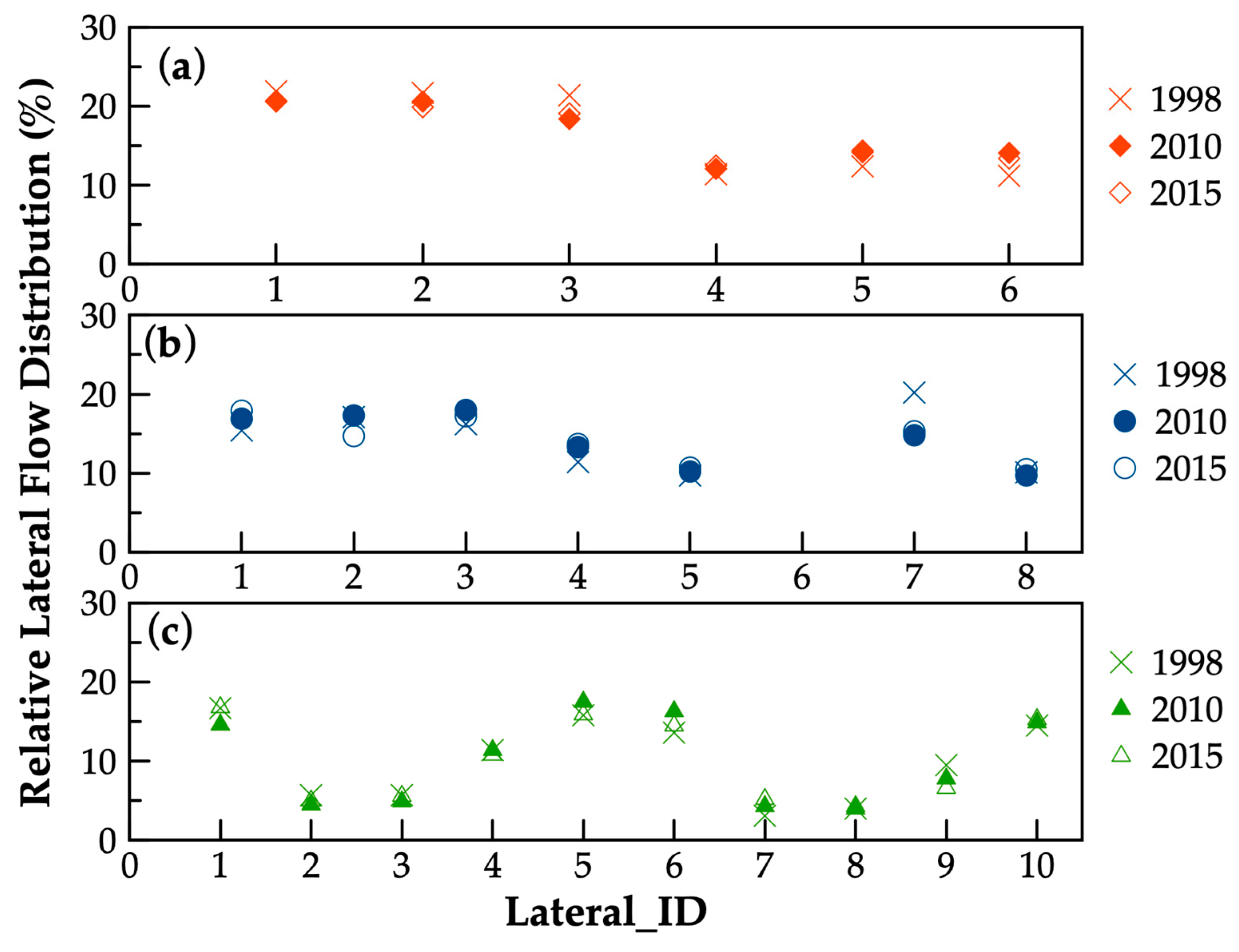
3.2. Lateral Flow Testing

The pumping levels in Collectors 3 and 4 had not stabilized after pumping (average rate ~0.6 m³ s⁻¹) for 1 week and for 4 days, respectively, and steady state conditions were not achieved. At the conclusion of this test pumping, Collector 3 was producing approximately 0.1 m³ s⁻¹ per m of observed drawdown. In contrast, at the end of testing in 2010, the collector well was producing about 0.14 m³ s⁻¹ per m of drawdown, suggesting a decline in performance of one-third in the intervening 5-year period. By adjusting the 2015 results and those from previous testings to be equivalent in terms of static water level and pumping water level, and without interference from the nearby Mirabel wellfield, the 2015 performance of Collector 3 is 3% lower than when it was originally constructed and tested in 1975, and approximately 10% lower than for the last previous inspection in 2010. By using similar adjustments, the 2015 performance of Collector 4 is about 23% better than it was in 2010, but 11% lower than its original performance after construction in 1975. On the other hand, the 2015 performance of Collector 5 has not changed substantially (±1%) [1,3].

Throughout the three investigations (1998, 2010, and 2015), minimal changes in relative percentage flow were observed (Figure 4). In Collector 3, the laterals (1, 2, and 3) closest to the river had the largest percentages of flow (Figure 4). The collective gain in flow in these three riverward laterals balances the collective loss of flow in the three landward laterals. During the 2015 evaluation, the relative distribution of flow among Collector 3 laterals ranged between 12.5 (Lateral 4) and 20.7% (Lateral 1). Lateral 6 had the largest decline in flow (−2.7%) compared to the 2010 results [1,3]. The limited changes observed may be related due to varying influence of recharge from the Russian River, as well as Infiltration Ponds 2 and 3 northeast and east of Collector 3 (Figure 2), respectively.

In Collector 4, during the three investigations, the productions of most of the laterals slightly improved over time. Laterals 1 and 2 (oriented toward the river) and Laterals 7 and 3 (parallel to the river) showed the highest percentages of flow. On the other hand, the lateral with the lowest percentage of flow (Lateral 8) is oriented on about a 45-degree angle towards the river, similar to Lateral 2, but it is also the shortest lateral (29.41 m) (Figure 2). The two landward laterals projected towards the infiltration ponds collectively provided 24.4% of the well’s total production. During the 2015 evaluation the relative flow percentages ranged between 10.5% (Lateral 8) to 17.9% (Lateral 1). Lateral 2 showed a decline (−2.5%) in production between 2010 and 2015 (Figure 2) [1,3]. Based on the video obtained, this decline was probably due to the presence of sand and gravel within the lateral.

In contrast with the trend observed in Collectors 3 and 4, in Collector 5, the laterals showed constrasting results. The production slightly increased in Laterals 1 and 7, slightly decreased in Laterals 4, 5, and 9, and remained constant in the remaining laterals. In addition, the impact of the 10 laterals is different. Four laterals individually procuded 14.5% or more of the total capacity, while five laterals individually produced less than 6.6% (Figure 4). The orientation of the laterals had no impact on the percentage of flow distributions. On the other hand, the length of the laterals impacted the flow distribution. The four longest laterals (>51.20 m) were also four of the five highest producing laterals, while the three shortest laterals (<26.52 m) were also the three lowest producing laterals. The three remaining laterals were of intermediate lengths (37.49 to 40.54 m), as well as in producing capability [1,3].

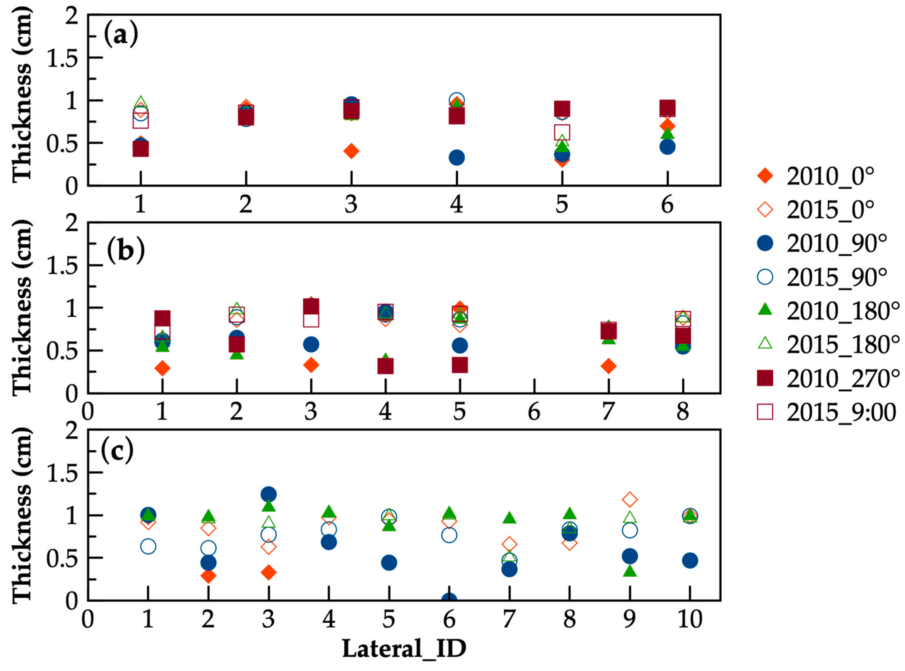
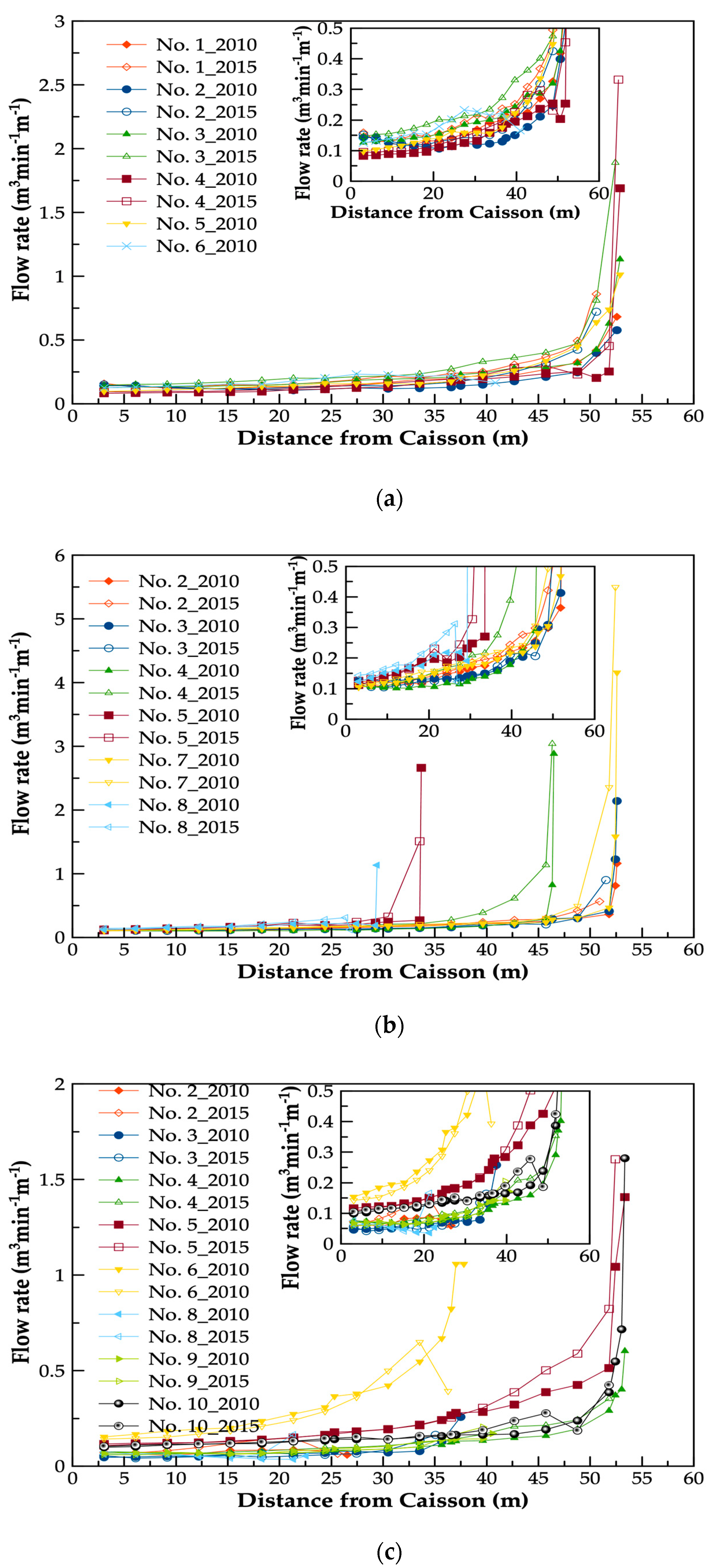
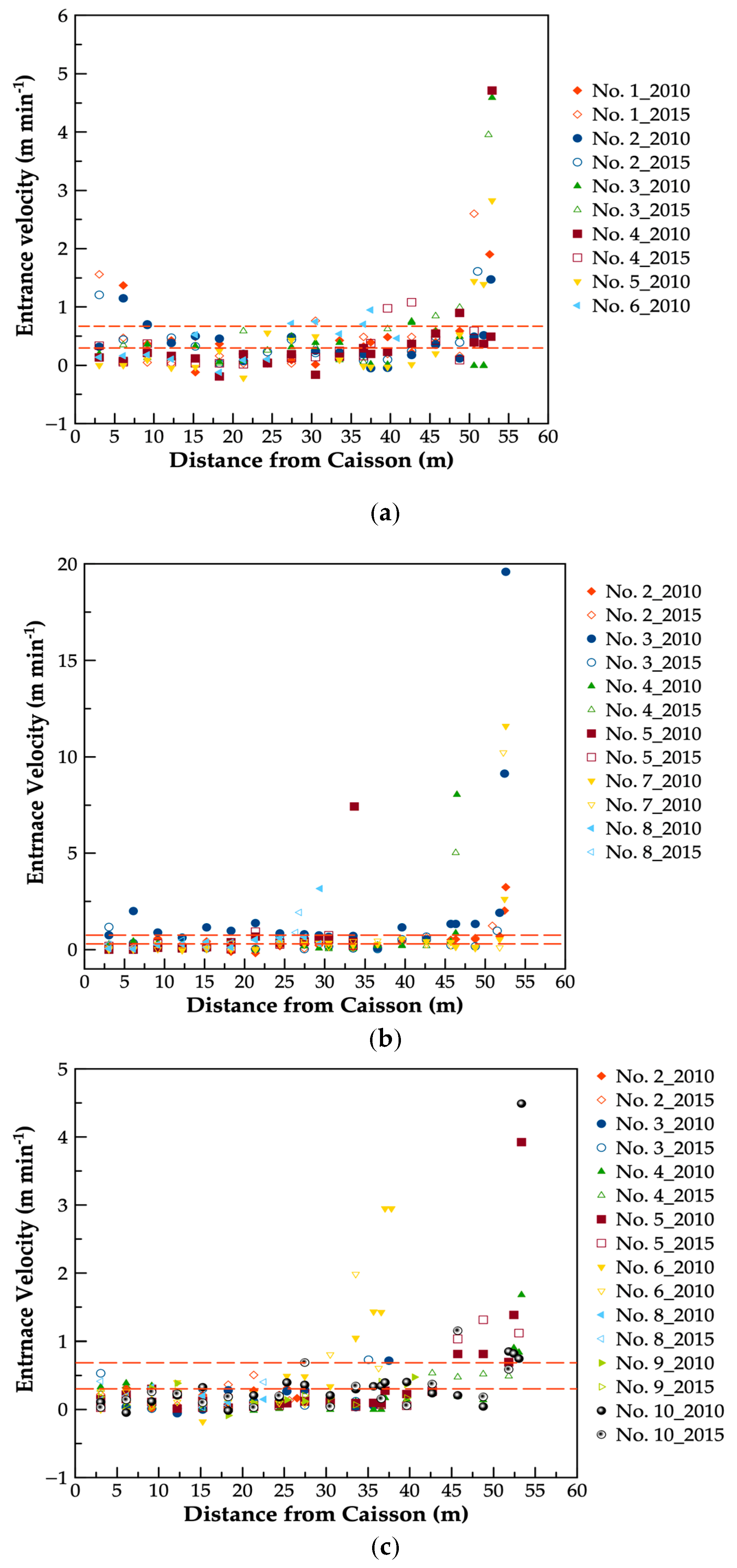
3.3. Lateral Flow Profiling

Non-uniform flow occurred along the laterals from the three collectors (Figure 5). In fact, for uniform flow along the lateral, the trend for each lateral would be a straight line beginning with zero m min⁻¹ at the outer end of the lateral and concluding with the total flow for the lateral where it enters the caisson. However, none of the laterals follow this straight-line trend of uniform distribution. Each lateral displays steeper gaining trends in production in the outermost segments of their length where they are obtaining most of their flow. After these steep gains in flow in the outer segments, the remaining trends of flow while moving progressively closer to the caisson were more gradual because of the generally slower production in those segments. Similar overall trends were observed during the 2010 and 2015 monitoring events. However, for Collector 3, regardless of the lateral, higher flow was observed during the 2015 campaign. On the other hand, for Collectors 4 and 5, a slightly higher flow was observed during the 2010 campaign [1,3].

Average unit flow capacity of each lateral, which is also greater at the end of lateral flow, effects large gains in production within only a few meters. This is particularly noticeable in Laterals 3 and 4 from Collector 3. In these outermost few feet, unit flow capacities can approach or even exceed 2 m³ min⁻¹ per m. On the other hand, while moving along the lateral toward the caisson, the gains in flow progressively decrease and the average unit flow capacity begins to assume a more consistent trend (Figure 6).

Overall, the three collectors are still within the optimal design parameters (entrance velocity < 0.305 m min⁻¹ and axial velocity < 1.524 m s⁻¹ [8,9]) (Figure 7 and Figure S3). Collector 6, constructed in 2002, consisted of a larger steel reinforced concrete caisson (5.49 m vs. 3.96 m inside diameter) with larger laterals (30.48 cm vs. 24. cm) than the Collectors discussed in this investigation, showed a lower entrance velocity (consistently < 0.610 m min⁻¹) and axial velocity (<1.524 m s⁻¹) during the 2010 monitoring campaign. This can also be related to lower presence of deposited materials and rust in Collector 6 (Figure S6) compared to the older collectors (Figure S2).

3.4. Water Quality

During the 2010 field campaign, the Russian River showed pH, EC, and DO values ranging between 7.5 and 8.5, between 190 and 240 μS cm⁻¹ and between 9 and 10 mg L⁻¹, respectively. During the same field campaign, similar pH and EC values were observed along the different laterals (Figure S4), while DO was consistently lower (Figure S5). Limited changes in terms of basic water quality parameters (i.e., pH, electrical conductivity, EC) were observed at three collectors during the two sampling campaigns, with more significant changes in dissolved oxygen (DO) and redox potential (ORP) (Figures S4 and S5). The pH ranged between 6.67 (Collector 3) and 7.31 (Collector 5) during the 2010 campaign, and between 6.78 (Collector 5) and 7.25 (Collector 3) during the 2015 campaign (Figure S5). Low EC (~220 μs cm⁻¹) were observed at the three collectors throughout the study (Figure S5). The DO was consistently lower during the 2015 campaign compared to the 2010 campaign. For example, at Collector 3, DO ranged from 3.5 to 7 mg L⁻¹ during the 2010 campaign and decreased during the 2015 campaign to a range between 1.5 and 6 3.5 to 7 mg L⁻¹ (Figure S5a). A similar but more pronounced trend was observed at Collectors 4 and 5 (Figure S5b,c). The ORP was also significantly different between the two sampling campaigns. In fact, ORP decreased over time at Collectors 4 and 5, and increased at Collector 3 (Figure S4). This different behavior in terms of DO and ORP may be related to the changes in temperature observed during the two investigations at the three collectors. Even if the two sampling campaigns were conducted during the same time of year (late October-early November), there was a difference in the river temperature. In particular, higher temperatures (~20.6 °C vs. 19.2 °C) were observed at Collector 4 during the 2015 campaing compared to the 2010 campaign. On the other hand, slightly warmer temperatures were observed during the 2015 campaign at Collectors 4 and 5 compared to the 2010 campaign [1,3].

4. Conclusions

This study highlights the performance of the three collector wells located over four decades. The field methods used during the 2010 and 2015 campaigns represented a valuable tool to evaluate the performance of collector wells regarding overall conditions, specific capacities, and entrance and axial velocities. Also, the impact of precipitation and consequently the variability of the river stage represent a key component for temporal comparisons. While water quality monitoring at the different laterals during the different campaigns are valuable information, basic river water quality parameters should also be monitored during these campaigns.

While Collectors 3 and 4 achieved lower performances compared with their original performances (1975), Collector 5 was relatively stable since 1982. The potential change in capacity could be due to the increase in encrustation observed during the visual inspection of laterals in all three collector wells. Overall, the three collectors are still within the optimal design parameters (screen entrance velocity < 0.305 m min⁻¹ and axial flow velocity of lateral screens < 1.524 m s⁻¹). The underwater structures in three collector wells are in generally good condition, early stages of rusting and encrustation are present. A more frequent cleaning and/or replacement of some of the rusted units may be required to further improve the efficiency of the collector wells.