Dynamic Modeling of Sediment Budget in Shihmen Reservoir Watershed in Taiwan

Abstract

Qualifying sediment dynamic in a reservoir watershed is essential for water resource management. This study proposed an integrated model of Grid-based Sediment Production and Transport Model (GSPTM) at watershed scale to evaluate the dynamic of sediment production and transport in the Shihmen Reservoir watershed in Taiwan. The GSPTM integrates several models, revealing landslide susceptibility and processes of rainfall–runoff, sediment production from landslide and soil erosion, debris flow and mass movement, and sediment transport. For modeling rainfall–runoff process, the tanks model gives surface runoff volume and soil water index as a hydrological parameter for a logistic regression-based landslide susceptibility model. Then, applying landslide model with a scaling relation of volume and area predicts landslide occurrence. The Universal Soil Loss Equation is then used for calculating soil erosion volume. Finally, incorporating runoff-routing algorithm and the Hunt’s model achieves the dynamical modeling of sediment transport. The landslide module was calibrated using a well-documented inventory during 10 heavy rainfall or typhoon events since 2004. A simulation of Typhoon Morakot event was performed to evaluate model’s performance. The results show the simulation agrees with the tendency of runoff and sediment discharge evolution with an acceptable overestimation of peak runoff, and predicts more precise sediment discharge than rating methods do. In addition, with clear distribution of sediment mass trapped in the mountainous area, the GSPTM also showed a sediment delivery ratio of 30% to quantify how much mass produced by landslide and soil erosion is still trapped in mountainous area. The GSPTM is verified to be useful and capable of modeling the dynamic of sediment production and transport at watershed level, and can provide useful information for sustainable development of Shihmen Reservoir watershed.

1. Background

Taiwan experiences frequent typhoons. It has steep mountains in fragmented geological settings from active tectonic motion-triggered earthquakes. Under intense rainfall, in the mountainsides, massive landslides often occur, triggering many debris flows and transporting huge amounts of sediment mass to downstream areas, which cause severe sediment problems and disasters (e.g., [1,2,3,4]). Some landslides with huge volumes of mass block river channels and form landslide dams. Under overtopping or internal erosion by upstream river water, these dams slowly breach and form sudden sedimentary or debris flow surges that strike downstream regions, destroying property, causing loss of human life, impacting use of general and hydraulic infrastructures, and causing so-called compound disasters, which greatly threatening all residents nearby and endanger Taiwanese society (e.g., [5]). Most landslide mass entering river channels lifts riverbed by deposition and then elevates the water level of river flow to cause flood inundations and serious damages to hydraulic infrastructures. When transported into reservoir area, all sediment load greatly raises sediment concentration, reducing water supply, increasing the trap efficiency and decreasing reservoir capacity and service lifetime by increasing bottom sedimentation (e.g., [6,7,8]). Particularly, in Taiwan, due to steep river inclination and short river length, reservoirs are the most important water resource infrastructure supplying water for livelihood, agriculture and industry. For the pursuit of sustainable development and disaster mitigation, the ability to model the dynamical sediment process in a reservoir watershed is required.

For modeling of watershed sediment dynamics, conventional methods mostly adopt rating curves of sediment load and discharge with imposed upstream boundary conditions and the only input is soil erosion, e.g., Hydrologic Engineering Center’s River Analysis System (HEC-RAS) [9], United States Environmental Protection Agency’s Hydrological Simulation Program-Fortran (HSPF) [10], and Soil and Water Assessment Tool (SWAT) [11]. It seems no conventional sediment routing models consider mass input from landslides and correctly reflect the spatiotemporal characteristic of landslide source in a watershed. However, in Taiwan, mass from hillslopes can greatly alter sediment amount in rivers, as it has been well evidenced that sediment volume dramatically increases after massive earthquakes and extreme rainfall [1,2,3]. Therefore, a model that integrates rainfall–runoff, landslide and soil erosion models for simulating mass production and movement with a dynamical model of riverbed erosion and sedimentation could facilitate simulation of all dynamic processes of rainfall-inducing hydrological response, mass production and movement, riverbed profile evolution, and sediment transportation in a watershed, and practically achieve precise prediction of watershed sediment budget by considering spatial property of sediment mass. In the past decades, great efforts have been made to successfully model or analyze the individual processes of rainfall–runoff (e.g., [12,13,14,15]), landslide prediction or movement (e.g., [16], and references therein), debris flow movement (e.g., [17,18,19,20,21,22,23]), dynamic sediment routing (e.g., [11,24], and references therein) and compound mass movement [25]. However, integrating all aforementioned models is quite challenging because of obvious differences of spatial and temporal scales among all processes. With some simplifications, some successful efforts have recently been made for similar issues (e.g., [26,27,28,29]). This present work aims to provide a new choice of grid-based model for modeling dynamic sediment budget and reflecting the spatiotemporal sediment mass feature.

To simulate watershed sediment dynamics considering landslides, this research proposes an integrated model Grid-based Sediment Production and Transport Model (GSPTM) by incorporating a several individual models for predicting landslide occurrence, and simulating mass production and movement, sediment transport, and river erosion and sedimentation from source area to downstream regions. The target area is Shihmen Reservoir watershed in northern Taiwan. First, landslide occurrence is estimated using a logistic regression-based landslide susceptibility model with time-varying soil water index (SWI) [30,31,32] and calculated by a conceptual tank model [33] under any given rainfall. Then, produced mass volume is estimated using empirical landslide volume–area relation [34] and the Universal Soil Loss Equation (USLE) [35] specifically calibrated for usage in Taiwan. Next, a method based on the Hunt’s model [36] is used to model the movement of mass from landslide and soil erosion. Finally, a calibrated hillslope runoff model [37] with sediment equilibrium concentration [38] simulates sediment movement. Details of each model are elaborated below. This integrated model was calibrated and tested on a well-documented event of severe Typhoons Morakot, by reconstructing the spatiotemporal distribution of sediment mass in the target area of Shihmen Reservoir watershed. The model is intentionally simplified due to lack of detailed information in a wider watershed, but it intends to provide valuable insights into sediment evolution under any hydrological forcing as a practical reference benefiting assessment of reservoir sedimentation and river channel safety.

2. Study Area—Shihmen Reservoir Watershed

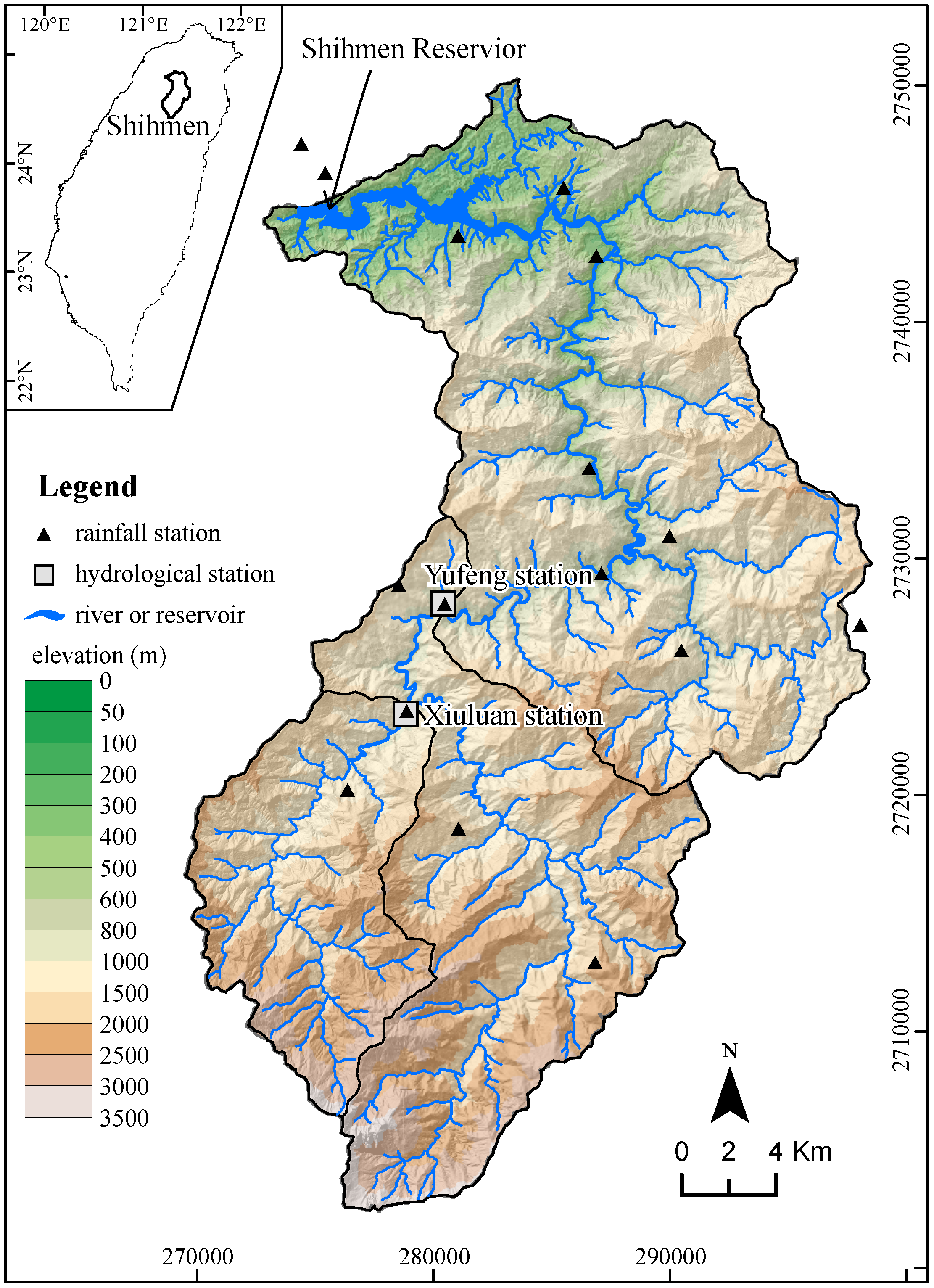
As shown in Figure 1, the Shihmen Reservoir is the third largest reservoir in Taiwan, and serves as the main source of public water supply for Taipei and Taoyuan cities in northern Taiwan. The reservoir has the total volume of 3.1 × 10${}^8$ m${}^3$ and the drainage area of 760 km${}^2$. In the reservoir watershed, the elevation ranges from 158 m (dam site) to 3524 m with an averaged slope of 26${}^{\circ }$. According to the delineation published by Water Resources Agency in Taiwan, the whole watershed is divided into seven official sub-watersheds: Xiuluan, Yufeng, Shankuang, Lengchiad, Kaoyi, Xiayun and Shihmen sub-watersheds. As explained below, this study focused on the most upstream Xiuluan and Yufeng watersheds, the total areas of which are 117.8 and 219.5 km${}^2$, respectively, as are marked in Figure 1. The geological setting mainly comprises sedimentary and low grade metamorphic rocks. The annual precipitation in this area reaches 2400 mm, and 70% of the total rainfall amount comes from the wet season, from May to September [39]. In the watershed, heavy rainfall often triggers landslides, soil erosion and debris flows. Transported by river flow, all these sediments finally reach the reservoir area to greatly increase the turbidity and trap efficiency of the reservoir, and decrease its storage capacity and service lifetime.

As illustrated in Figure 2, from 2004 to 2013, ten rainfall events brought a great amount of landslides in this watershed, and, particularly, the most massive landslides were caused by Typhoon Aere in 2004 [34]. Reaching a cumulative amount of 997 mm, the intense rainfall from Typhoon Aere totally triggered 6.01 km${}^2$ of landslide area [34]. Then, huge amount of high concentration runoff flowed to the reservoir, causing sediment silting in a volume of approximately 2.7 × 10${}^7$ m${}^3$ [40]. After this typhoon, significant quantity of sediment that remained in upstream rivers [41] was continuously transported into the reservoir by subsequent rainfall, and considerably raised the turbidity of Shihmen Reservoir. Since then, the reservoir authority has been working on resolving the sediment problem through various countermeasures in the past decade (e.g., [8,41]). Sustainable water resources management demands reliable and precise information of sediment dynamic in a reservoir watershed under any hydrological forcing, which is what the GSPTM can model.

3. Introduction to GSPTM

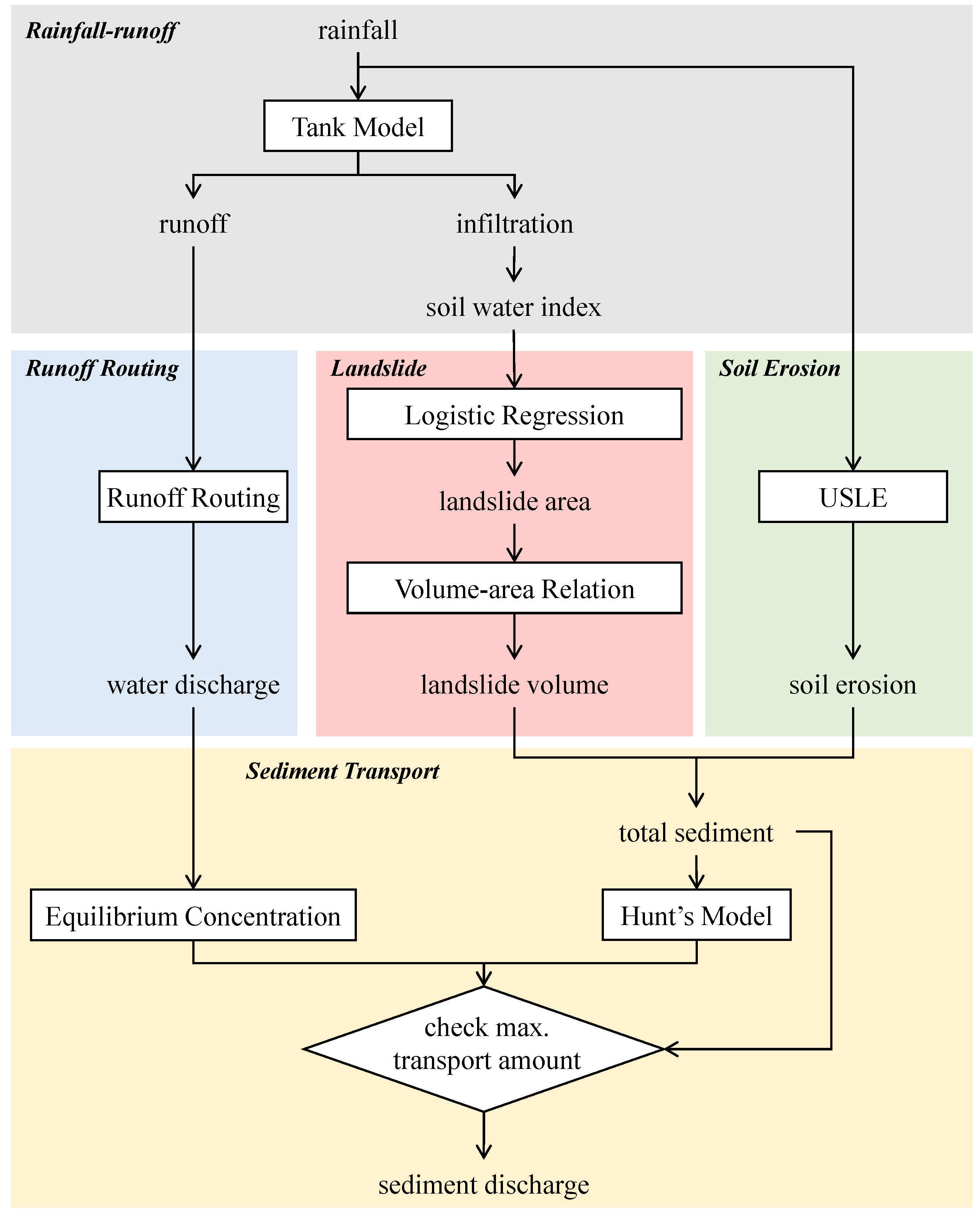
Figure 3 illustrates the GSPTM framework, comprising five modules for modeling rainfall–runoff, landslide, soil erosion, runoff-routing, and sediment transport processes, respectively. The calculation flow starts by modeling of rainfall-inducing runoff and infiltration using the conventional tank model. In the second step, the infiltration part, called soil water index (SWI), is taken as a hydrological parameter in the logistic regression model that predicts landslide area. Then, landslide volume is calculated by using the area predicted with a landslide volume–area relation. The third step adopts USLE to estimate the soil erosion volume. The fourth step is to obtain the runoff on hillslopes and in river channels by a grid-based routing algorithm. Finally, with the simulated runoff, the transport processes of the sediment from landslide and soil erosion are, respectively, simulated by equilibrium concentration theory and Hunt’s model in a grid-based algorithm. A detailed description of each module is elaborated in the following.

Particularly, as a distributed type model, the GSPTM can output all simulated variables of time variation at any location in the target watershed, and flexibly set any sink or source on grids of interest for any possible application. For efficient computation among five modules and GIS data, GSPTM was implemented using Matlab, which has comprehensive and well-developed libraries. All computation procedures were completed in Matlab.

3.1. Rainfall–Runoff Model

The rainfall–runoff process is simulated by using the tank model, a conceptual model for flood routing [33]. By assuming hillslope surface, and shallow and deep soil layers as three tanks, the tank model can calculate water storage in and vertical movement among the three tanks from surface infiltration under a given rainfall event. When storage in a tank exceeds the tank’s capacity, the excess amount becomes the outflow volumetric discharge in the corresponding soil layer. The tank model generates three storages, i.e., $S_1$, $S_2$ and $S_3$, reflecting water volumes on hillslope surface and in shallow and deep soil layers, and also gives three outflows, i.e., $q_1$, $q_2$ and $q_3$, representing the volumetric discharge of surface runoff contributed by each soil layer. The storages $S_2$ and $S_3$ can qualitatively reflect the soil moisture condition in the corresponding layers, and can be considered as a factor representing hillslope stability. Thus, based on this concept, the soil water index (SWI) is defined as the summation of all storages, i.e., $swi=S_1+S_2+S_3$, and is being used as an index for early-warning assessment of landslide and debris flow hazards in Japan (e.g., [30,31,42]) and Taiwan (e.g., [32] and references therein).

According to the successful verification and analysis of Taiwanese cases [43], the GSPTM directly follows the literature to adopt the conventional tank model with original parameters [33], and uses $swi$ for landslide prediction and $Q=q_1+q_2+q_3$ as water volumetric discharge on hillslope surface for runoff-routing.

3.2. Sediment Production Prediction

3.2.1. Landslide Model

The landslide module adopts a logistic regression model to predict the landslide area and estimate landslide volume by a scaling volume–area relation with the area predicted. Logistic regression analysis, also called binary regression analysis, is a widely used statistical model when the dependent variable is binary, e.g., landslide occurrence or nonoccurrence, and independent variables are in the numerical type (e.g., slope), in the categorical type (e.g., lithology), or in both types (e.g., [44]). As it is beyond the present paper’s scope, some detailed verification of applying the logistic regression model to landslide prediction can be referred to in the literature (e.g., [45,46,47]).

In the GSPTM, the logistic regression model follows the form

$$\begin{array}{c}\hfill \begin{array}{cc}\hfill Logit(y)& =a+\sum b_i{x}_i+e,\hfill \\ \hfill P& ={[1+exp\left(-Logit(y)\right)]}^{-1},\hfill \end{array}\end{array}$$

(1)

where $exp(·)$ denotes the exponential function, y is the independent variable, $x_i$ are the explanatory variables, a and $b_i$ are the coefficients, e is the error term, and P is the probability of landslide occurrence. To calibrate the logistic regression model for landslide prediction, the explanatory variables include elevation, slope, aspect, profile and plane curvatures, Topographic Wetness Index (TWI), distances to river, ridge, and road, lithology and SWI. To represent topographic effects, the common variables of elevation, slope, aspect and curvatures are generated using a 40-m digital elevation model (DEM). The aspect variable is taken by sine and cosine functions to represent the east–west and north–south vectors, respectively. The profile and plane curvatures indicate the surface concavity of a hillslope grid in the longitudinal and planar directions. The TWI variable represents the spatial distributions of soil moisture and surface saturation [48] determined by taking natural logarithm of the ratio of specific contributing area, i.e., total contributing area divided by contour length, to slope. The distances from a location to the nearest river, ridge and road are used to quantify how the three influences landslide occurrence. The lithology is a categorized variable indicating the rock properties, such as rock strength, joint density, and so on. Finally, the SWI can represent pore-water pressure variation in soil or rock.

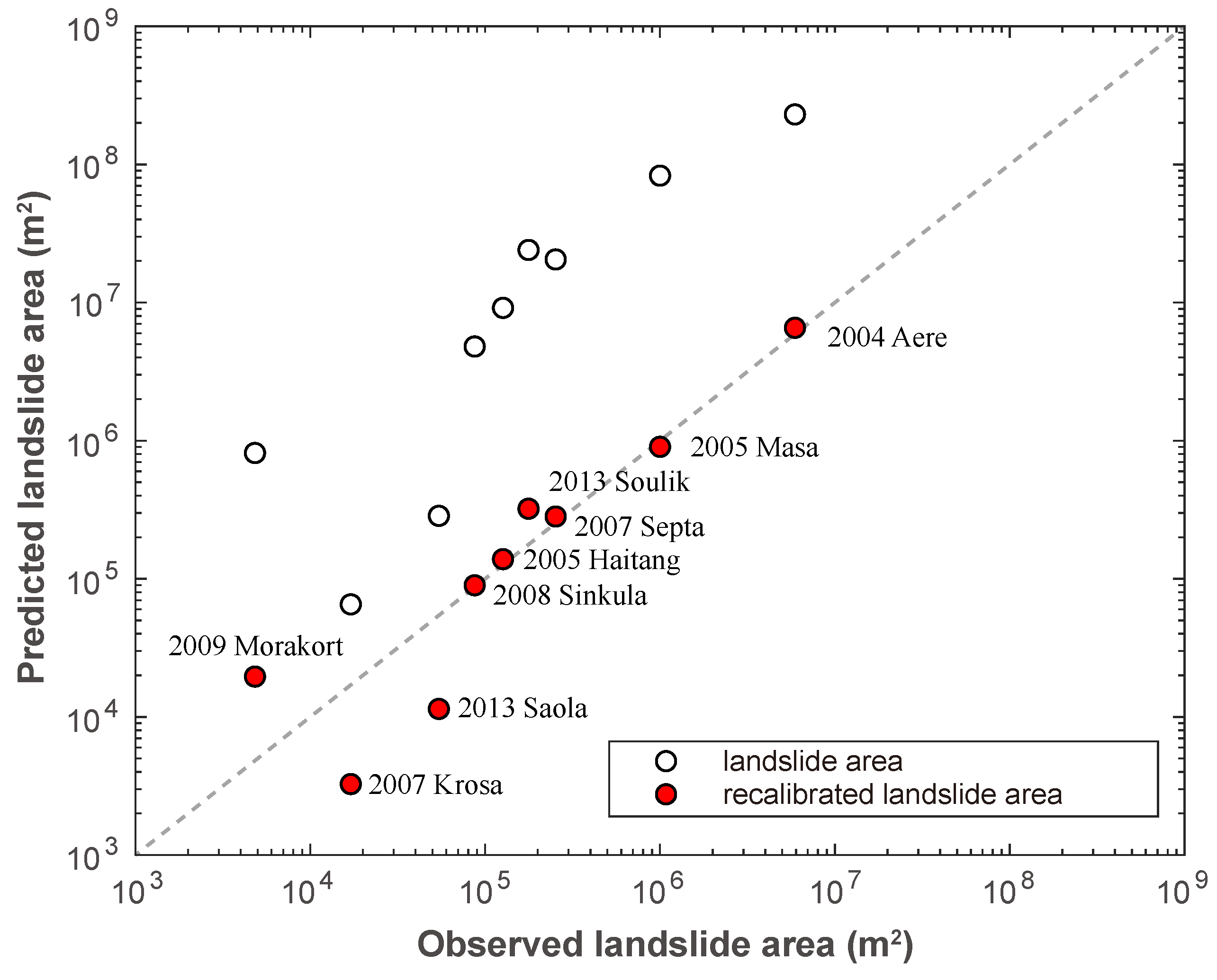
To determine all variable coefficients, the calibration adopted the largest landslide events brought by Typhoon Aere in 2004. Particularly, the constant a and the coefficient for SWI were recalibrated by comparing the observed and predicted landslide area using the inventory of nine typhoons to avoid overestimation of landslide area. The recalibration results are plotted in Figure 4, and the correct prediction ratio for landslide occurrence and nonoccurrence are 74.3% and 70.5%, respectively. These successful ratios indicate the logistic landslide model is acceptable and quite correct for predicting landslide location. For Shihmen Reservoir watershed, the logistic regression function is expressed as

$$\begin{array}{c}\begin{array}{cc}Logit(y)=\hfill & -8.0\times {10}^{-4}\mathit{ele}+0.058\mathit{slp}+0.076\mathit{aps}-0.45\mathit{apc}-1.84\mathit{cpf}-1.67\mathit{cpl}+0.25\mathit{twi}\hfill \\ & -9.0\times {10}^{-4}\mathit{drv}+5.0\times {10}^{-3}\mathit{drd}+4.0\times {10}^{-5}\mathit{dro}+\mathit{geo}+0.00657\mathit{swi}-7.534,\hfill \end{array}\end{array}$$

(2)

where $\mathit{ele}$ is the topographic elevation (m); $\mathit{slp}$ is the slope gradient (${}^{\circ }$); $\mathit{aps}$ and $\mathit{apc}$ are, respectively, the sine and cosine of aspects (-); $\mathit{cpf}$ and $\mathit{cpl}$ are the profile and plane curvatures (-); $\mathit{twi}$ is the topographic wetness index (-); $\mathit{drv}$, $\mathit{drd}$ and $\mathit{dro}$ denote the distances to river, ridge and road (m), respectively; $\mathit{geo}$ represents the lithological type; and $\mathit{swi}$ is the soil water index (SWI) (mm). All calibrated coefficients and relating statistical properties are tabulated in

Table 1. Logistic regression coefficients and the significance level of explanatory variables.

Attribute (unit)	Variable	Coefficient b	Standard Error of the Mean (%)	Wald	p-Value
elevation (m)	$\mathit{ele}$	8.0 × ${10}^{-4}$	0.000	106.810	0.000
inclination (${}^{\circ }$)	$\mathit{slp}$	0.058	0.002	554.326	0.000
aspect sine (-)	$\mathit{aps}$	0.076	0.028	7.211	0.007
aspect cosine (-)	$\mathit{apc}$	−0.45	0.028	274.032	0.000
longitudinal curvature (m${}^{-1}$)	$\mathit{cpf}$	−1.84	0.710	6.740	0.009
planar curvature (m${}^{-1}$)	$\mathit{cpl}$	−1.67	0.684	5.942	0.015
topographic wetting index (m)	$\mathit{twi}$	0.25	0.016	245.940	0.000
distance to river (km)	$\mathit{drv}$	−9.0 × ${10}^{-4}$	0.000	58.786	0.000
distance to ridge (km)	$\mathit{drd}$	5.0 × ${10}^{-3}$	0.000	27.411	0.000
distance to road (km)	$\mathit{dro}$	4.0 × ${10}^{-5}$	0.000	8.967	0.003
geological category ${}^{†}$	$\mathit{geo}$	1.0	0.000	106.810	0.000
soil water index (m)	$\mathit{swi}$	0.00657	0.000	985.196	0.000
constant (-)	$\mathit{a}$	−7.534	0.275	695.069	0.000

${}^{†}$ Values for various lithological types refer to Table 2.

and

Table 2. Regression values for the categorical variable of $geo$ in terms of different lithological types.

Category	Value	Category	Value
Erhchiu formation (Eh)	−0.297	Kangkou formation (Kk)	−1.008
Tapu Formation (Tp)	1.271	Tsuku Formation (Tu)	−0.175
Mushan Form (Ms)	0.237	Terrace Deposits (t)	−2.302
Paling Form (Pl)	0.714	Piling Shale (Pi)	0.000
Peiliao Formation (Pe)	0.136	Shihti Formation (St)	−0.058
Szeleng Sandstone (Ss)	−0.158	Hsitsun Formation (Ht)	−0.300

. Then, landslide occurrence probability P can be determined through the obtained $Logit(y)$.

With the landslide area predicted by the logistic model (Equations (1) and (2)), GSPTM estimates the corresponding landslide volume through a scaling relationship between landslide volume $V_L$ and area $A_L$. As clearly explained in the literature [49], a landslide volume–area relation can interpret a given landslide area for a reasonable corresponding volume. For shallow landslides, the scaling exponent in the relation is often less than 1.3; otherwise, deep-seated landslides usually have a power greater than 1.3. Using the samples of 20 landslides near or in the watershed, the fitting relationship was obtained using a robust regression that is not vulnerable to outliers and can prevent bias of outcomes [34]. With the samples in Dahan River watershed, the volume–area relationship is given by

$$\begin{array}{c}\hfill V_L=0.458\times A_L^{1.179},R^2=0.94,\end{array}$$

(3)

where $V_L$ is the landslide volume (m${}^3$) and $A_L$ is the landslide area (m${}^2$). With a high determination coefficient $R^2=0.94$, Equation (3) can provide a significant and highly-explanatory estimate of landslide volume through a given area in Shihmen Reservoir watershed. Note that $V_L=0$ on grids where landslide prediction is nonoccurrence. Moreover, the scaling exponent of 1.179 reflects that the landslide type is shallow one.

3.2.2. Soil Erosion Prediction

The GSPTM uses the USLE to estimate sediment volume from soil erosion,

$$\begin{array}{c}\hfill V_S=R_m\times K_m\times K\times S\times C\times P,\end{array}$$

(4)

where $V_S$ is the soil loss (t ha${}^{-1}$), $R_m$ is the rainfall erosivity factor (MJ mm ha${}^{-1}$ h${}^{-1}$), $K_m$ is the soil erodibility factor (t h MJ${}^{-1}$ mm${}^{-1}$), L and S are the topographic factors (-), and C and P are the crop management and conservation practice factors (-). The following explanation introduces how we obtained each factor in Equation (4) specific for the Shihmen Reservoir watershed. However, for other watersheds, all factors can be easily obtained in a similar way. One can also refer to other ways for soil erosion estimation (e.g., [50]).

Wischmeier and Smith [51] found that soil erosion is highly correlated with the multiplication of the cumulative rainfall energy and maximum 30-min rainfall intensity. Thus, the rainfall erosivity factor $R_m$ can be expressed as

$$\begin{array}{c}\hfill R_m=I_{30}\times \sum _{i=1}^n\left(E_k\times I_k\right),\end{array}$$

where $I_{30}$ is the maximum 30-min cumulative rainfall intensity (mm h${}^{-1}$), $I_k$ is the kth hour rainfall amount (mm h${}^{-1}$), and $E_k$ is the kth unit rainfall energy (M J mm${}^{-1}$ ha${}^{-1}$), which is calculated by

$$\begin{array}{c}\hfill E_k=\left\{\begin{array}{cc}0.119+0.0873{log}_{10}{I}_k,\hfill & \mathrm{for}{I}_k\le 76\mathrm{mm}/\mathrm{h},\hfill \\ 0.283,\hfill & \mathrm{for}{I}_k>76\mathrm{mm}/\mathrm{h}.\hfill \end{array}\right.\end{array}$$

Because it is readily available from meteorological gauge stations, the maximum hourly rainfall was multiplied by 1.5 to represent the $I_{30}$ [52]. Then, to obtain the rainfall erosivity index for Shihmen Reservoir watershed, the $I_{30}$ were determined by 40 m × 40 m rainfall distributions interpolated by the rainfall data from 16 gauge stations, of which the locations are marked by black triangles in Figure 1.

For the topograhic factors, the slope length L is calculated by

$$\begin{array}{c}\hfill L={(x/22.13)}^m,\end{array}$$

where x is the runoff flow length (m) that denotes the flow distance from a ridge [53]. McCool et al. [54] suggested the slope factor S specific for steep slops can be calculated by

$$\begin{array}{c}\hfill S=\left\{\begin{array}{cc}10.3sin\theta +0.03,\hfill & \mathrm{for}\theta <9\%,\hfill \\ {(sin\theta /0.0896)}^{0.6},\hfill & \mathrm{for}\theta \ge 9\%,\hfill \end{array}\right.\end{array}$$

where $\theta$ is the slope gradient.

Finally, the soil erodibility factor $K_S$ and cropping management factors, C and P, were determined through soil and land-use maps with the reference tables in [55,56]. With Equation (4), all sediment produced by soil erosion at each 40 m × 40 m grid can be obtained for sediment transport calculation, which is introduced in Section 3.5.

3.3. Mass Movement Simulation

For modeling movement of mass produced by landslides and soil erosion, the GSPTM simulates two processes of debris flow and runoff-driven sediment transport. Firstly, the GSPTM adopts the Hunt’s model [36] that simulates debris flow process as a steady and fully-developed laminar flow in terms of a 40 m × 40 m grid. Even quite simplified without revealing the complex initiation and flowing processes of real debris flows, the approach can efficiently capture reasonable debris flow movement in a wider simulation area (e.g., [57]). As it is a very thin soil–water mixture flow, the movement of the mass produced by soil erosion is simulated using the same method as for modeling debris flow. By, respectively, imposing no-slip and stress-free boundary conditions on the bottom and free surface, the velocity profile of debris flow is given as

$$\begin{array}{c}\hfill u_M(z)=\frac{gsin\theta }{2\nu }\left(h_M^2-{(h_M-z)}^2\right),\end{array}$$

(5)

where $u_M$ is the flow velocity (m s${}^{-1}$), z is the spatial variable in the vertical direction (m), $h_M$ is the flow depth (m), $\nu$ is the kinematic viscosity (m${}^2$ s${}^{-1}$), g is the gravitational acceleration (m s${}^{-2}$), and $\theta$ is the average slope inclination (${}^{\circ }$). Particularly, as an essential factor, debris flow viscosity $\nu$ can be determined through precise calibration method [58]. Here, we referred to relevant literature [57] when setting it to be $\nu =0.25$. Integrating Equation (5) from the channel bed to flow surface gives the discharge of well-developed debris flow

$$\begin{array}{c}\hfill Q_M={\int }_0^{h_M}{u}_M\mathrm{d}z=\frac{g{h}_M^{3}sin\theta }{3\nu },\end{array}$$

(6)

where the flow depth $h_M$ at the $(k+1)$-time is readily determined by

$$\begin{array}{c}\hfill h_M^{k+1}=h_M^k+\frac{1}{\Delta X^2}(V_L^k+V_S^k),\end{array}$$

where $V_L$ and $V_S$ are, respectively, obtained from Equations (3) and (4) at the k-time, and $\Delta X$ is the grid length and $\Delta X=40$ m in this study. During model calculation, $V_L=0$ on grids where landslide prediction is nonoccurrence or when rainfall stops.

To calculate $Q_M$ at a grid $(i,j)$, the algorithm first searches grids having lover $h_M$ in eight adjacent grids $(i\pm 1,j\pm 1)$ and calculates corresponding $Q_M$. Then, the algorithm determines outflows in multiple flow directions to the adjacent grids having lower water levels, but constrains the outflow in each direction by multiplying a weighting factor that represents the ratio of the outflow in the direction to the total outflows in all direction to prevent from violating $h_M$ conservation by over outflow from the center grid $(i,j)$. Afterwards, mass movement obtained from $Q_M$ calculation is used as an input for sediment transport modeling.

3.4. Runoff Simulation

In the whole watershed, runoff-routing simulation was based on a grid-based distributed model that can model the hydrological process of overland flow everywhere in mainstream and its tributaries, and represent the spatial distribution of environmental variables of interest, e.g., hillslope runoff for sediment transport modelling. For runoff-routing modeling with the surface runoff obtained by the tank model, the GSPTM adopts the following conservation equation

$$\begin{array}{c}\hfill \Delta S/\Delta t=I-Q,\end{array}$$

where I is the inflow (m${}^3$ s${}^{-1}$), Q is the outflow (m${}^3$ s${}^{-1}$), $\Delta S$ is the storage change (m${}^3$), and $\Delta t$ is the time interval (s). With the application of the simplified model [37], the runoff-routing algorithm separately treats surface runoff in the streams and on the hillslope. A main difference for hillslope and stream channel can be regarded as the drainage contributing area. Obtained by using the D-infinity flow direction algorithm [59,60], the drainage contributing area $A_c$ is used to distinguish the hillslope and stream channel grid by a threshold of $0.2$ km${}^2$, and

$$\begin{array}{c}\hfill \mathrm{grid}(i,j)=\left\{\begin{array}{cc}\mathrm{hillslope},\hfill & \mathrm{if}{A}_c\le 0.2{\mathrm{km}}^2,\\ \mathrm{stream}\mathrm{channel},\hfill & \mathrm{if}{A}_c>0.2{\mathrm{km}}^2.\end{array}\right.\end{array}$$

(7)

On a stream channel grid $(i,j)$, assumed as a rectangular open channel, the runoff discharge is calculated by the Manning equation in a discrete form as below,

$$\begin{array}{c}\hfill Q_{ij}=\frac{B{H}_H}{n_{ij}}{\left(\frac{B{H}_H}{B+2H_H}\right)}^{2/3}{\left(\frac{(Z_H-Z_L)+(H_H-H_L)}{\Delta X}\right)}^{1/2},\end{array}$$

(8)

where $Q_{ij}$ is the runoff volume flowing to the downstream (m${}^3$ s${}^{-1}$) and $(i,j)$ denotes the grid indices in the $(x,y)$ directions, $n_{ij}$ is the Manning’s coefficient ranging from 0.035 to 0.050 in terms of each grid’s surface roughness [61] or land-use condition, and B is the stream width (m) calculated from the empirical relation between stream width and contributing area [62]. $H_H$ and $H_L$, respectively, denote the higher and lower water levels (m), and $Z_H$ and $Z_L$ are the higher and lower riverbed elevations (m) between two adjacent grids. Again, $\Delta X$ is the distance between two grids (m).

On the other hand, for calculating runoff on a hillslope grid $(i,j)$, by reasonably ignoring the energy loss due to shallow flow motion, the runoff discharge is given as

$$\begin{array}{c}\hfill Q_{ij}=\frac{B{H}_H^{5/3}}{n_{ij}}{\left(\frac{(Z_H-Z_L)+(H_H-H_L)}{\Delta X}\right)}^{1/2}.\end{array}$$

(9)

Both the $Q_{ij}$ in Equations (8) and (9) follow a similar multiple flow direction algorithm introduced in Section 3.3. For runoff or overland flow calculation at a grid $(i,j)$, the algorithm first searches grids having lover water levels in eight adjacent grids $(i\pm 1,j\pm 1)$ and calculates corresponding hydraulic slopes in terms of 40 m × 40 m DEM. Again, each outflow is multiplied by a specific weighting factor, determined by a similar way as in Section 3.3, to ensure conservation property of outflow from the center grid $(i,j)$. Afterwards, the runoff obtained is used for modeling the sediment transport process.

3.5. Sediment Transport

The GSPTM simulates runoff-driven sediment transport by anticipating the surface runoff Q obtained by runoff simulation and the sediment equilibrium concentration $C_{d\infty }$ [38] that estimates maximum capacity of sediment transport under a given slope inclination,

$$\begin{array}{c}\hfill C_{d\infty }=exp\left(1.73ln\theta -5.83\right),\end{array}$$

(10)

where $C_{d\infty }$ denotes the maximum sedimentary concentration and $C_{d\infty }\in [0,1]$, and $\theta$ is the longitudinal riverbed inclination. The empirical relation above is based on experiments with a high correlation of 97% [63], and is very useful for routing sediment in mountainous area where information of sediment grain size is usually unavailable. Then, at each grid $(i,j)$, the index subscripts are omitted hereafter for clarity, with Equations (6) and (10), the total sedimentary discharge is calculated by

$$\begin{array}{c}\hfill Q_T=Q_C+Q_M,\end{array}$$

(11)

where $Q_C=Q\times C_{d\infty }$ is the maximum capacity of runoff-driven sediment transport and Q is the runoff discharge obtained from Equation (8) or (9) in terms of the grid type. $Q_T$ represents the sediment transport contributed by surface runoff, landslide and soil erosion. However, to satisfy conservation property, the final sediment discharge $Q_S$ (t s${}^{-1}$) is checked by the maximum mass amount from landslide and soil erosion, i.e., $Q_{max}=\Delta X^2{h}_M$, as below

$$\begin{array}{c}\hfill Q_S=\left\{\begin{array}{cc}{Q}_T,& \mathrm{if}{Q}_T\le Q_{max},\\ Q_{max},& \mathrm{if}{Q}_T>Q_{max},\end{array}\right.\end{array}$$

(12)

If $Q_T\le Q_{max}$ exists, the excess sediment mass deposits in the grid, thus elevating the surface.

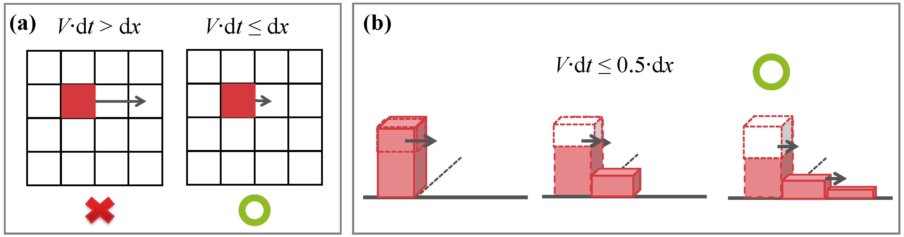
Finally, for stable computation of advection processes, the GSPTM adopts stability conditions that restrict an appropriate time increment, as illustrated in Figure 5. Analogous to the famous Courant–Friedrichs–Lewy (CFL) condition, the model flexibly adjusts the time increment to prevent the condition that advection spans over the eight adjacent grids, i.e., $V\mathrm{d}t>\mathrm{d}x$ in Figure 5a, and, based on our experience, the advection is stable when $V\mathrm{d}t\le 0.5\mathrm{d}x$ in Figure 5b. As one usually accepts that the maximum velocity of landslide or debris flow is about 20 m/s on mountainsides, the GSPTM suggests a minimum time increment of 1 s for a 40 m × 40 m grid that is temporally fine enough for modeling dynamic sediment movement.

3.6. Model Verification and Performance Elevation

The landslide module, i.e., Equations (1)–(3), was verified using the inventory from ten typhoons, as shown in Figure 2 and Figure 4. To evaluate the GSPTM’s performance, we simulated the sediment movement during Typhoon Morakot in 2009 and verified simulated runoff discharge and sediment concentration with field measurements at Xiuluan and Yufeng stations, where the locations are marked in Figure 1.

4. Result and Discussion—Reconstruction of Typhoon Morakot Event

In 2009, Typhoon Morakot stroke Taiwan during 7–9 August, drawing great amount of water vapor from Indian monsoon to bring record-breaking rainfall, with the maximum five-day cumulative rainfall reaching 3004.5 mm in southern Taiwan, and triggered massive landslides in mountainous area. During the typhoon, landslides catastrophically destroyed transportation and water power and supply infrastructures. Some of the huge landslide mass deposited and trapped in mountainous area, and then caused other disasters or damages again during sequential rainfall events. As mentioned aboe, to achieve sustainable development of Shihmen Reservoir, the authority not only routinely maintains reservoir area by dredging, but aims to resolve landslide problems to ensure soil conservation in the watershed upstream regions. For the later goal, we used GSPTM to reveal the spatial distribution of landslide mass and corresponding sediment transport in Shihmen Reservoir watershed under an extreme weather event of Typhoon Morakot.

According to Tsai et al. [41], the ratio of the total landslide volume in Yufeng and Xiuluan watersheds to the one in the whole Shihmen Reservoir watershed reached 46.7% from 1968 to 1975, 62.2% from 1976 to 1985, 59.2% from 1986 to 1997, 40.5% from 1998 to 2003, and 61.7% from Typhoon Aere in 2004. Contributing more than half of total volume, the Xiuluan and Yufeng watersheds are the main mass sources of landslide in Shihmen Reservoir watershed. Thus, in the following, we only present the simulated results of the two watersheds, including landslide prediction, sediment transport and turbidity, and sediment delivery ratio.

4.1. Mass Production by Landslide and Soil Erosion

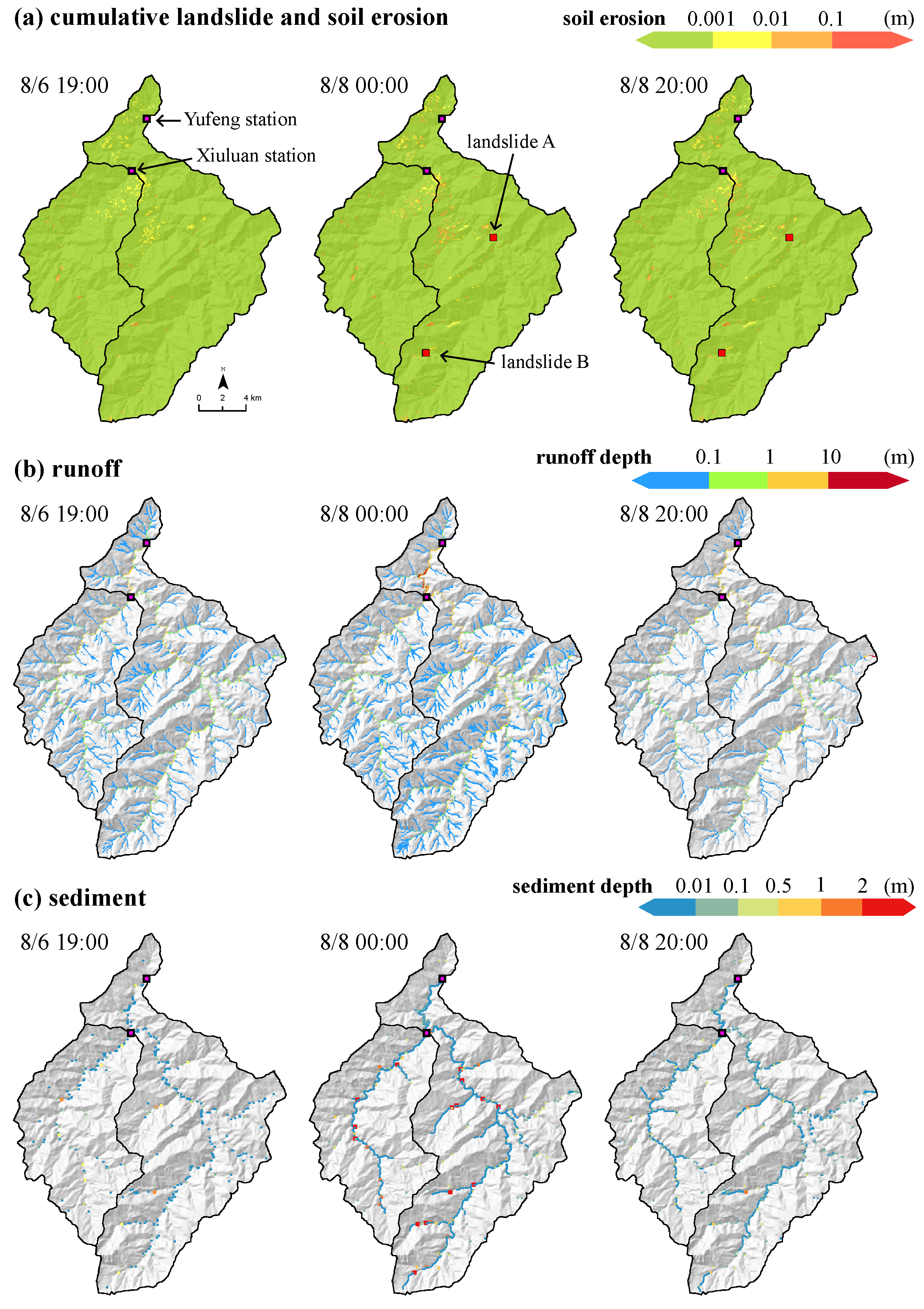
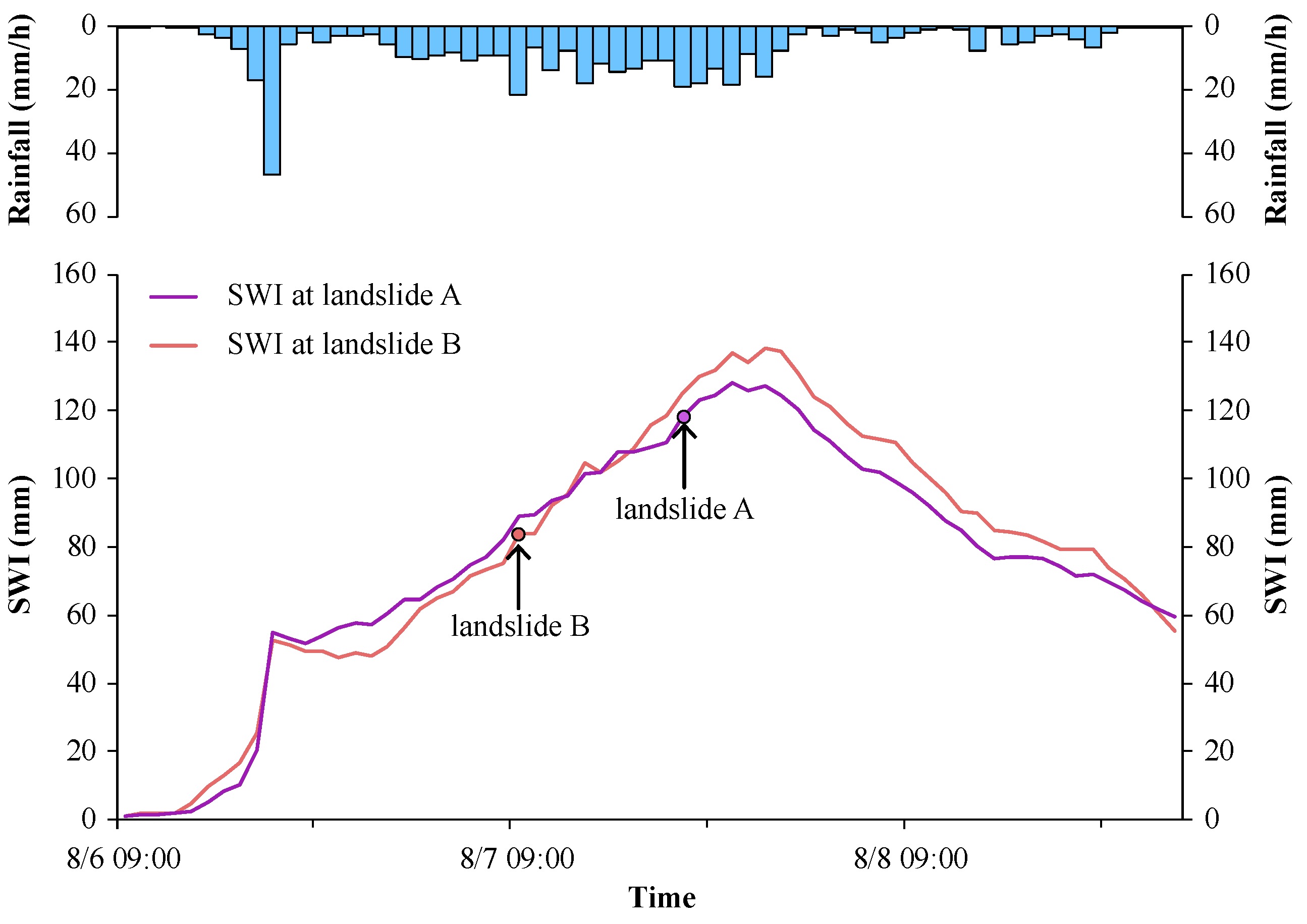
In this case, the GSPTM predicted two landslides occurred at 0:00 on 8 August, (UTC+8 time zone hereafter), in the upstream region of Yufeng watershed, and the occurrence locations are marked by red rectangles in Figure 6a. The landslide volumes are 3384 and 7315 m${}^3$, respectively. Figure 7 illustrates how rainfall and simulated SWI affect occurrence of the two landslides A and B in Figure 6a. The obvious increasing tendency of SWI appears both at the two landslide sites. Particularly, the logistic landslide model predicted occurrence in the middle of the increasing SWI curves, not at the peaks. In addition, the predicted occurrence locations are close to the places of past hazards in the inventory, as in Figure 2. Both these conditions evidence that the GSPTM can provide reasonable prediction of mass production from landslide and soil erosion.

Figure 6a illustrates prediction of mass distribution produced by soil erosion and two landslides. The simulation indicates soil erosion generated more cumulative mass than landslide did. For the spatial distribution, it is obvious that soil erosion dominated and almost reached 0.1 m at the place nearby Xiuluan station in Yufeng watershed, and reached a total volume of 8.2 × 10${}^5$ t, as shown in Figure 8c,d. As is the main purpose of this model, the results verify the GSPTM can provide the time-varying spatial distribution of sediment mass from landslide and soil erosion.

4.2. Sediment Transport Condition

The main objective of GSPTM is to simulate sediment movement considering spatially-relating processes of landslide and soil erosion. The simulated spatial distributions of runoff and sediment from landslide and soil erosion at three instants of 19:00 on 6 August, and 0:00 and 20:00 on 8 August are clearly illustrated in Figure 6b,c. In what follows, the simulation shows excellent prediction of peak discharge timing and sediment discharge volume, but fair prediction of runoff discharge.

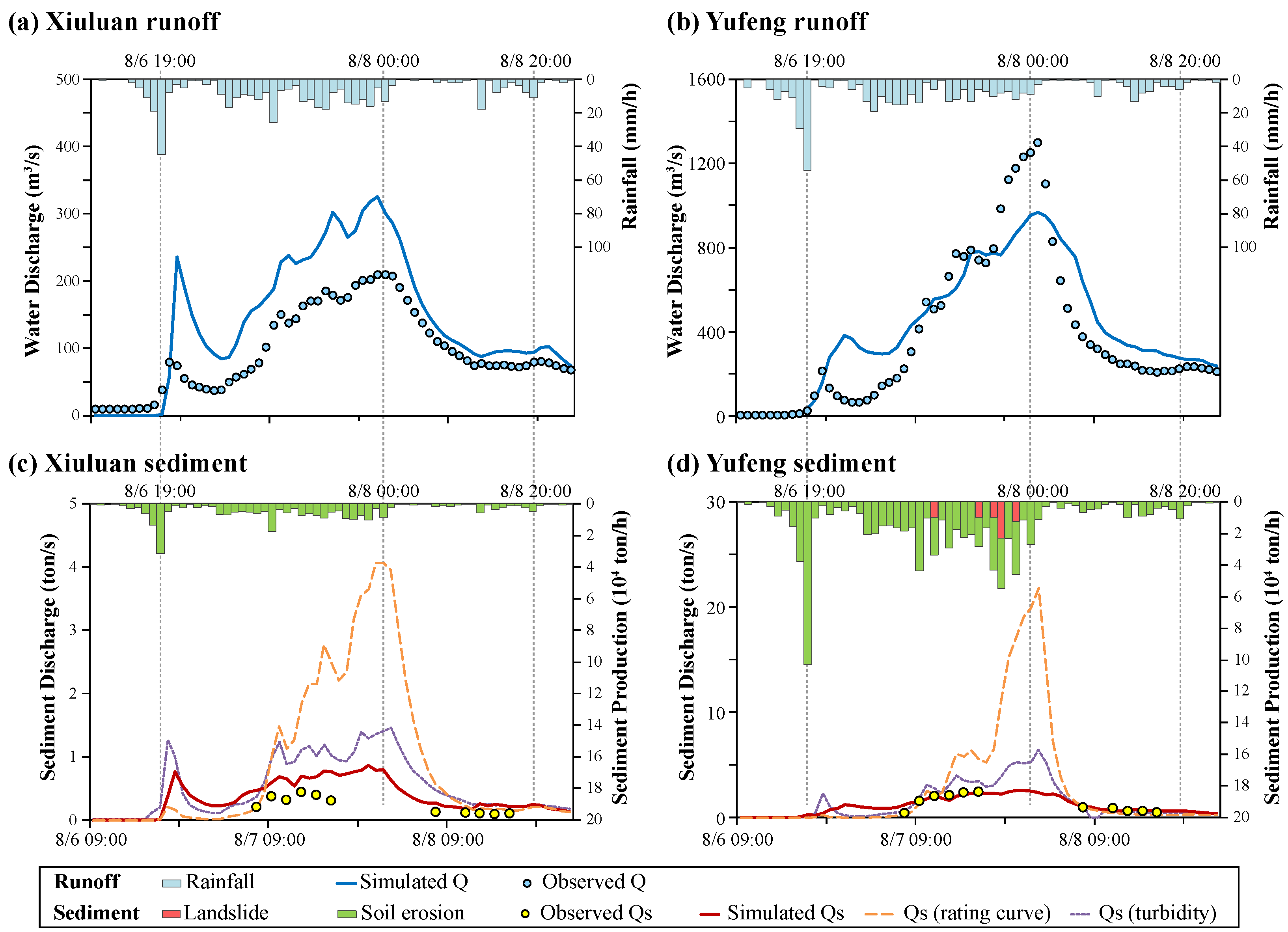
With the simulated hydrographs of runoff and sediment discharge, Figure 8 illustrates comparison between simulated results and field measurements at Yufeng and Xiuluan gauge stations. The simulated runoff in both cases captures the tendency of the measured one, but has sightly overestimated peak values by 56% at Xiuluan station, and underestimated peak values by −26% at Yufeng station, as shown in Figure 8a,b. These runoff over- and underestimates may come from the outflows of rainfall–runoff modeling, and could be resolved by further parameter calibration of the tank model. However, the runoff tendency was precisely revealed by only using the grid-based runoff simulation algorithm in Section 3.4. At Xiuluan station, the observed peak runoff discharge occurred at 23:00 on 7 August, and the simulated one was at the same time. Besides, at Yufeng station, both observed and simulate peak runoff discharges also happened at 01:00 on 8 August. Even having an allowable discharge overestimation, the GSPTM can exactly model the runoff tendency in this case.

The most significant part is that the GSPTM model provides a rather correct prediction of sediment concentration compared to the one using the conventional sediment rating method. For comparing with simulation, three variables were used: (1) observed $Q_S$ by using direct sampling of sediment concentration [64] at each station; (2) turbidity $Q_S$ by direct sensor measurement and laboratory analysis [64]; and (3) rating $Q_S$ by measured flow rate with rating curves. In Figure 8c, the peak discharge of simulated $Q_S$ occurred at 22:00 on 7 August, and then followed by the rating $Q_S$ and turbidity $Q_S$ at 23:00 and 01:00 on 8 August. The simulated one happened just one hour in advance of the field condition. However, the sediment discharges have huge variations starting at 07:00 on 7 August. The rating $Q_S$ obtained by the most conventional method had a quite high peak discharge that is almost 3.4 and 8.3 times of the turbidity $Q_S$ and simulated $Q_S$, respectively. It is obvious the simulated $Q_S$ best fits the the most precise observed $Q_S$. At Yufeng station, the peak discharge of simulated $Q_S$ also first occurred at 23:00 on 7 August, followed by the rating $Q_S$ and turbidity $Q_S$ at 01:00 on 8 August. Particularly, the simulated $Q_S$ coincides with the observed one very well starting from 09:00 on 7 August but the rating and turbidity $Q_S$ still greatly diverge from the observed. This reflects that the GSPTM successfully simulated the sediment discharge.

4.3. Sediment Delivery Condition

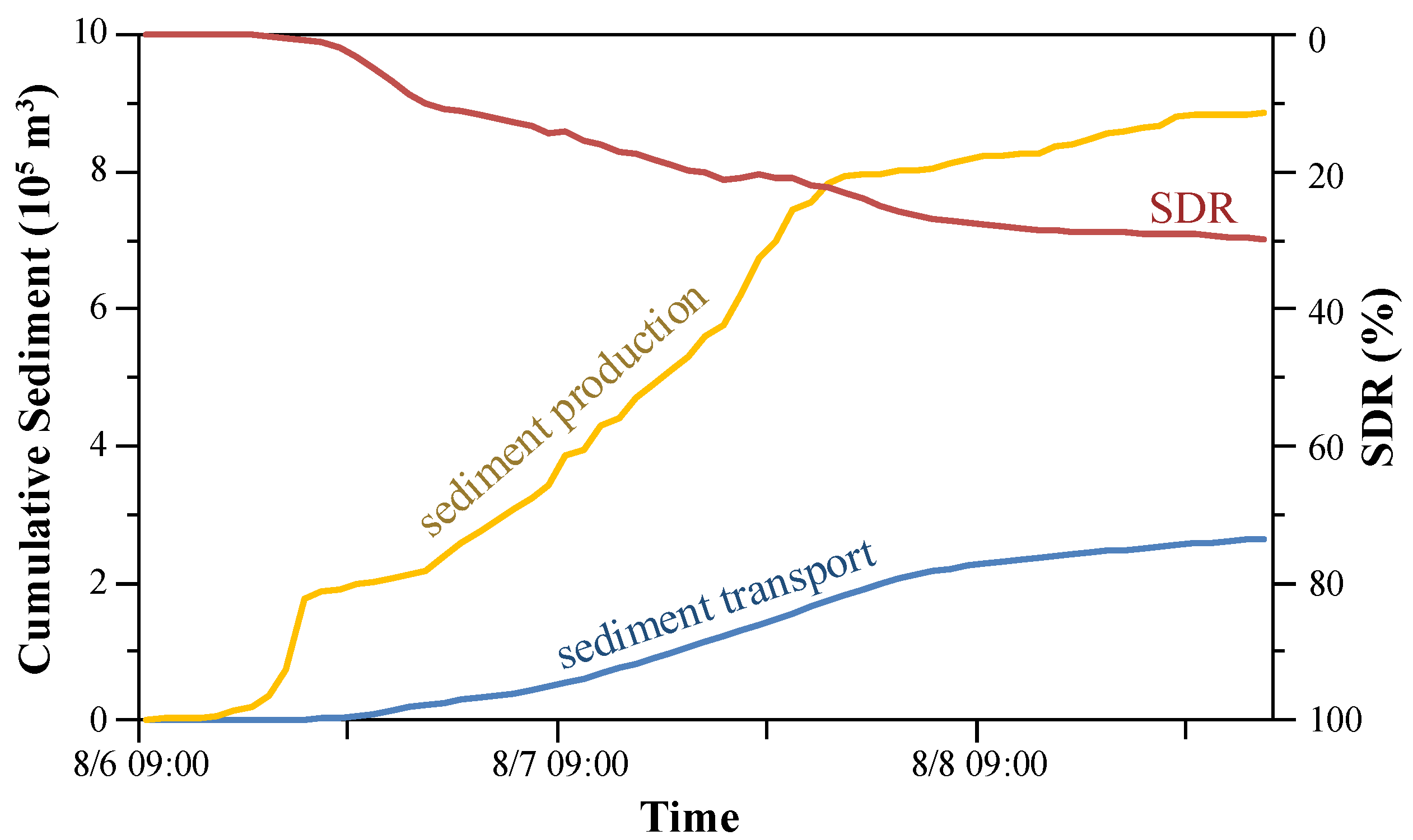
For soil conservation planning, the sediment delivery condition plays an essential role as the reference index. As mentioned in the previous section, the spatial distributions of sediment mass are readily obtained from simulation. For an overview of total transport quantity in the whole watershed, the other reference is the chart of sediment delivery ratio (SDR) representing the total transported sediment volume to the total production volume, as shown in Figure 9. The total cumulative sediment production reached about 8.86 × 10${}^5$ t, of which the transported total sediment was only 2.65 × 10${}^5$ t. This means that only about 29.91% of sediment mass was transported to downstream regions, while 70.09% remained in Yufeng and Xiuluan watersheds. The simulated SDR exactly coincides with the typical value [65]. The significance is that, without any empirical relation, the GSPTM directly simulated a reasonable estimate of SDR in this case.

Shen et al. [66] reported that the total volume of residual sediment mass was still 53% three years after Typhoon Morakot. By sequential rainfall or typhoons, this huge amount of residual sediment mass could be detached to form other sedimentary problems, and influence the watershed ecosystem and infrastructures in downstream regions. Again, this emphasizes the importance of obtaining the SDR information and its modeling capability for disaster prevention and sustainable development.

5. Concluding Remarks

To improve conventional sediment rating methods for sediment budget assessment, we proposed the Grid-base Sediment Production and Transport Model (GSPTM) for directly modeling sediment dynamics in a wide watershed considering spatial distributions of landslide and soil erosion. The event of Typhoon Morakot was re-investigated for performance evaluation. By comparing with measurements from Xiuluan and Yufeng gauge stations, the simulation successfully reconstructed more accurate sediment discharge hydrographs than the rating ones. In addition, the typical sediment delivery ratio of 30% was obtained without any empirical relation. These results verify the GSPTM’s capability and validity for spatiotemporally revealing sediment dynamics in a wide watershed. However, as one point to improve, the runoff simulation over- and underestimated at the two gauge stations in the case analysis, but this problem could be fixed by improving the tank model through further parameter calibration.

Through the modeling methodology proposed, we can gain insights into how dynamical sediment movement occurs and influences sediment concentration in Shihmen Reservoir. The GSPTM’s output of mass distribution is evidenced to be a valuable reference for the reservoir authority to plan future soil conservation engineering. Furthermore, without a lot of effort, the GSPTM can be easily extended to other watershed of interest, and provide precise assessment of sediment budget under any given rainfall input of any engineering or scientific interest.

References

- Dadson, S.J.; Hovius, N.; Chen, H.; Dade, W.B.; Lin, J.C.; Hsu, M.L.; Lin, C.W.; Horng, M.J.; Chen, T.C.; Milliman, J.; et al. Earthquake-triggered increase in sediment delivery from an active mountain belt. Geology 2004, 32, 733–736. [Google Scholar] [CrossRef]
- Kao, S.J.; Lee, T.Y.; Milliman, J.D. Calculating highly fluctuated suspended sediment fluxes from mountainous rivers in Taiwan. Terr. Atmos. Ocean. Sci. 2005, 16, 653. [Google Scholar] [CrossRef]
- Lin, Y.; Chen, Y.; Lee, H. The budget of sediment supply and removal triggered by typhoon tainfall in the Kaoping river basin. In Proceedings of the 2013 APEC Typhoon Symposium, Taipei, Taiwan, 21–23 October 2013; pp. 21–23. [Google Scholar]
- Chen, Y.C.; Chang, K.T.; Lee, H.Y.; Chiang, S.H. Average landslide erosion rate at the watershed scale in southern Taiwan estimated from magnitude and frequency of rainfall. Geomorphology 2015, 228, 756–764. [Google Scholar] [CrossRef]
- Dong, J.J.; Lai, P.J.; Chang, C.P.; Yang, S.H.; Yeh, K.C.; Liao, J.J.; Pan, Y.W. Deriving landslide dam geometry from remote sensing images for the rapid assessment of critical parameters related to dam-breach hazards. Landslides 2014, 11, 93–105. [Google Scholar] [CrossRef]
- Lin, G.W.; Chen, H.; Petley, D.N.; Horng, M.J.; Wu, S.J.; Chuang, B. Impact of rainstorm-triggered landslides on high turbidity in a mountain reservoir. Eng. Geol. 2011, 117, 97–103. [Google Scholar] [CrossRef]
- Kondolf, G.M.; Gao, Y.; Annandale, G.W.; Morris, G.L.; Jiang, E.; Zhang, J.; Cao, Y.; Carling, P.; Fu, K.; Guo, Q.; et al. Sustainable sediment management in reservoirs and regulated rivers: Experiences from five continents. Earths Future 2014, 2, 256–280. [Google Scholar] [CrossRef]
- Wang, H.W.; Kondolf, M.; Tullos, D.; Kuo, W.C. Sediment management in Taiwan’s reservoirs and barriers to implementation. Water 2018, 10, 1034. [Google Scholar] [CrossRef]
- Brunner, G.W. HEC-RAS 5.0 Users Manual; US Army Corps of Engineers, Institute for Water Resources, Hydrologic Engineering Center: Washington, DC, USA, 2016. [Google Scholar]
- Lee, H.Y.; Lin, Y.T.; Chiu, Y.J. Quantitative estimation of reservoir sedimentation from three typhoon events. J. Hydrol. Eng. 2006, 11, 362–370. [Google Scholar] [CrossRef]
- Krysanova, V.; Arnold, J.G. Advances in ecohydrological modelling with SWAT—A review. Hydrol. Sci. J. 2008, 53, 939–947. [Google Scholar] [CrossRef]
- Chow, V.T.; Maidment, D.R.; Larry, W. Applied Hydrology; MacGraw-Hill: New York, NY, USA, 1988. [Google Scholar]
- Brutsaert, W. Hydrology: An Introduction; Cambridge University Press: Cambridge, UK, 2005. [Google Scholar]
- Sayama, T.; McDonnell, J.J. A new time-space accounting scheme to predict stream water residence time and hydrograph source components at the watershed scale. Water Resour. Res. 2009, 45, W07401. [Google Scholar] [CrossRef]
- Sayama, T.; Ozawa, G.; Kawakami, T.; Nabesaka, S.; Fukami, K. Rainfall–runoff–inundation analysis of the 2010 Pakistan flood in the Kabul River basin. Hydrol. Sci. J. 2012, 57, 298–312. [Google Scholar] [CrossRef] [Green Version]
- Chae, B.G.; Park, H.J.; Catani, F.; Simoni, A.; Berti, M. Landslide prediction, monitoring and early warning: A concise review of state-of-the-art. Geosci. J. 2017, 21, 1033–1070. [Google Scholar] [CrossRef]
- Wu, Y.H.; Liu, K.F.; Chen, Y.C. Comparison between FLO-2D and Debris-2D on the application of assessment of granular debris flow hazards with case study. J. Mt. Sci. 2013, 10, 293–304. [Google Scholar] [CrossRef]
- Wu, Y.H.; Liu, K.F. The Influence of Countermeasure on Debris Flow Hazards with Numerical Simulation. In Landslide Science for a Safer Geoenvironment; Sassa, K., Canuti, P., Yin, Y., Eds.; Springer: Cham, Switzerland, 2014; pp. 473–478. [Google Scholar]
- Han, Z.; Chen, G.; Li, Y.; Xu, L.; Zheng, L.; Zhang, Y. A new approach for analyzing the velocity distribution of debris flows at typical cross-sections. Nat. Hazards 2014, 74, 2053–2070. [Google Scholar] [CrossRef]
- Liu, K.F.; Wei, S.C.; Wu, Y.H. The influence of accumulated precipitation on debris flow hazard area. In Landslide Science for a Safer Geoenvironment; Springer: Berlin, Germany, 2014; pp. 45–50. [Google Scholar]
- Iverson, R.M.; George, D.L. A depth-averaged debris-flow model that includes the effects of evolving dilatancy. I. Physical basis. Proc. R. Soc. A 2014, 470, 20130819. [Google Scholar] [CrossRef]
- George, D.L.; Iverson, R.M. A depth-averaged debris-flow model that includes the effects of evolving dilatancy. II. Numerical predictions and experimental tests. Proc. R. Soc. A 2014, 470, 20130820. [Google Scholar] [CrossRef]
- Han, Z.; Chen, G.; Li, Y.; Tang, C.; Xu, L.; He, Y.; Huang, X.; Wang, W. Numerical simulation of debris-flow behavior incorporating a dynamic method for estimating the entrainment. Eng. Geol. 2015, 190, 52–64. [Google Scholar] [CrossRef]
- Papanicolaou, A.T.N.; Elhakeem, M.; Krallis, G.; Prakash, S.; Edinger, J. Sediment transport modeling review—Current and future developments. J. Hydraul. Eng. 2008, 134, 1–14. [Google Scholar] [CrossRef]
- Iverson, R.M.; Ouyang, C. Entrainment of bed material by Earth-surface mass flows: Review and reformulation of depth-integrated theory. Rev. Geophys. 2015, 53, 27–58. [Google Scholar] [CrossRef] [Green Version]
- Alatorre, L.; Beguería, S.; García-Ruiz, J. Regional scale modeling of hillslope sediment delivery: A case study in the Barasona Reservoir watershed (Spain) using WATEM/SEDEM. J. Hydrol. 2010, 391, 109–123. [Google Scholar] [CrossRef] [Green Version]
- Easton, Z.M.; Fuka, D.R.; White, E.D.; Collick, A.S.; Biruk Ashagre, B.; McCartney, M.; Awulachew, S.B.; Ahmed, A.A.; Steenhuis, T.S. A multi basin SWAT model analysis of runoff and sedimentation in the Blue Nile, Ethiopia. Hydrol. Earth Syst. Sci. 2010, 14, 1827–1841. [Google Scholar] [CrossRef] [Green Version]
- Liu, K.F.; Wu, Y.H.; Chen, Y.C.; Chiu, Y.J.; Shih, S.S. Large-scale simulation of watershed mass transport: A case study of Tsengwen reservoir watershed, southwest Taiwan. Nat. Hazards 2013, 67, 855–867. [Google Scholar] [CrossRef]
- Kabir, M.A.; Dutta, D.; Hironaka, S. Estimating sediment budget at a river basin scale using a process-based distributed modelling approach. Water Resour. Manag. 2014, 28, 4143–4160. [Google Scholar] [CrossRef]
- Okada, K. Soil water index. Sokkojihou 2002, 69, 67–100. [Google Scholar]
- Osanai, N.; Shimizu, T.; Kuramoto, K.; Kojima, S.; Noro, T. Japanese early-warning for debris flows and slope failures using rainfall indices with Radial Basis Function Network. Landslides 2010, 7, 325–338. [Google Scholar] [CrossRef]
- Chen, S.; Tsai, C.; Chen, C.; Chen, M. Soil Water Index applied as a debris flow warning-reference based on a tank model. J. Chin. Soil Water Conserv. 2013, 44, 31–43. [Google Scholar]
- Ishihara, Y.; Kobatake, S. Runoff model for flood forecasting. Bull. Disaster Prev. Res. Inst. 1979, 29, 27–43. [Google Scholar]
- Chen, Y.C.; Chang, K.T.; Chiu, Y.J.; Lau, S.M.; Lee, H.Y. Quantifying rainfall controls on catchment-scale landslide erosion in Taiwan. Earth Surf. Proc. Land. 2013, 38, 372–382. [Google Scholar] [CrossRef]
- Williams, J.; Berndt, H. Sediment yield prediction based on watershed hydrology. Trans. ASAE 1977, 20, 1100–1104. [Google Scholar] [CrossRef]
- Hunt, B. Newtonian fluid mechanics treatment of debris flows and avalanches. J. Hydraul. Eng. ASCE 1994, 120, 1350–1363. [Google Scholar] [CrossRef]
- Yeh, T.T. Simulation on the Rainfall–Runoff Process in Shihmen Watershed. Master’s Thesis, National Central University, Taoyuan, Taiwan, 2003. [Google Scholar]
- Takahashi, T. Debris flow. Annu. Rev. Fluid Mech. 1981, 13, 57–77. [Google Scholar] [CrossRef]
- Water Resource Agency. Hydrological Yearbook, 2008 Part I: Rainfall; Technical Report; Water Resource Agency, Ministry of Economic Affair: Taipei, Taiwan, 2009. [Google Scholar]
- Northern Region Water Resource Office. Evaluation of Morphological Effects in Downstream River due to Sediment Venting and Replenishment from the Shihmen Reservoir, Taoyuan; Technical Report; Water Resources Agency, Ministry of Economic Affairs: Taipei, Taiwan, 2014. [Google Scholar]
- Tsai, Z.X.; You, G.J.Y.; Lee, H.Y.; Chiu, Y.J. Modeling the sediment yield from landslides in the Shihmen Reservoir watershed, Taiwan. Earth Surf. Proc. Land. 2013, 38, 661–674. [Google Scholar] [CrossRef]
- Saito, H.; Matsuyama, H. Catastrophic landslide disasters triggered by record-breaking rainfall in Japan: Their accurate detection with Normalized Soil Water Index in the Kii Peninsula for the year 2011. Sci. Online Lett. Atmos. 2012, 8, 81–84. [Google Scholar] [CrossRef]
- Chen, C.W.; Oguchi, T.; Hayakawa, Y.S.; Saito, H.; Chen, H.; Lin, G.W.; Wei, L.W.; Chao, Y.C. Sediment yield during typhoon events in relation to landslides, rainfall, and catchment areas in Taiwan. Geomorphology 2018, 303, 540–548. [Google Scholar] [CrossRef]
- Menard, S. Applied Logistic Regression Analysis; Sage: Thousand Oaks, CA, USA, 2002; Volume 106. [Google Scholar]
- Chang, K.T.; Chiang, S.H.; Hsu, M.L. Modeling typhoon-and earthquake-induced landslides in a mountainous watershed using logistic regression. Geomorphology 2007, 89, 335–347. [Google Scholar] [CrossRef]
- Chang, K.T.; Chiang, S.H. An integrated model for predicting rainfall-induced landslides. Geomorphology 2009, 105, 366–373. [Google Scholar] [CrossRef]
- Chan, H.C.; Chen, P.A.; Lee, J.T. Rainfall-induced landslide susceptibility using a rainfall–runoff model and logistic regression. Water 2018, 10, 1354. [Google Scholar] [CrossRef]
- Beven, K.J.; Kirkby, M.J. A physically based, variable contributing area model of basin hydrology/Un modèle à base physique de zone d’appel variable de l’hydrologie du bassin versant. Hydrol. Sci. J. 1979, 24, 43–69. [Google Scholar] [CrossRef]
- Larsen, I.J.; Montgomery, D.R.; Korup, O. Landslide erosion controlled by hillslope material. Nat. Geosci. 2010, 3, 247. [Google Scholar] [CrossRef]
- Liu, Y.H.; Li, D.H.; Chen, W.; Lin, B.S.; Seeboonruang, U.; Tsai, F. Soil erosion modeling and comparison using slope units and grid cells in Shihmen reservoir watershed in northern Taiwan. Water 2018, 10, 1387. [Google Scholar] [CrossRef]
- Wischmeier, W.H.; Smith, D.D. Rainfall energy and its relationship to soil loss. Eos Trans. Am. Geophys. Union 1958, 39, 285–291. [Google Scholar] [CrossRef]
- Yang, S.; Jan, C.; Huang, C.; Tseng, K. Application of hourly rainfall data to estimate the rainfall erosion index. J. Chin. Soil Water Conserv. 2010, 41, 189–199. [Google Scholar]
- Lin, C.Y.; Lin, W.T.; Chou, W.C. Soil erosion prediction and sediment yield estimation: The Taiwan experience. Soil Tillage Res. 2002, 68, 143–152. [Google Scholar] [CrossRef]
- McCool, D.; Brown, L.; Foster, G.; Mutchler, C.; Meyer, L. Revised slope steepness factor for the Universal Soil Loss Equation. Trans. ASAE 1987, 30, 1387–1396. [Google Scholar] [CrossRef]
- Hsieh, Z.; Wang, M. An Atlas Major Soils of Taiwan; Soil Survey and Testing Center, National Chung Hsing University: Taichung, Taiwan, 1991. [Google Scholar]
- Lee, C. Soil and Water Conservation Handbook; Soil and Water Conservation Bureau: Nantou, Taiwan, 2017. [Google Scholar]
- Chiang, S.H.; Chang, K.T.; Mondini, A.C.; Tsai, B.W.; Chen, C.Y. Simulation of event-based landslides and debris flows at watershed level. Geomorphology 2012, 138, 306–318. [Google Scholar] [CrossRef]
- Wu, Y.H.; Liu, K.F. Formulas for calibration of rheological parameters of bingham fluid in couette rheometer. J. Fluids Eng. 2015, 137, 041202. [Google Scholar] [CrossRef]
- Tarboton, D.G. A new method for the determination of flow directions and upslope areas in grid digital elevation models. Water Resour. Res. 1997, 33, 309–319. [Google Scholar] [CrossRef] [Green Version]
- Yang, T.H.; Chen, Y.C.; Chang, Y.C.; Yang, S.C.; Ho, J.Y. Comparison of different grid cell ordering approaches in a simplified inundation model. Water 2015, 7, 438–454. [Google Scholar] [CrossRef]
- Chow, V.T. Open-Channel Hydraulics; McGraw-Hill: New York, NY, USA, 1959. [Google Scholar]
- Leopold, L.B.; Wolman, M.G.; Miller, J.P. Fluvial Processes in Geomorphology; Courier Corporation: Chelmsford, MA, USA, 2012. [Google Scholar]
- Tsai, Y.F.; Shieh, C.L. Experimental and numerical studies on the morphological similarity of debris-flow fans. J. Chin. Inst. Eng. 1997, 20, 629–642. [Google Scholar] [CrossRef]
- Northern Region Water Resource Office. Artificial and Automatic Monitoring for Water Quality at Shihmen Reservoir and Watershed, Taoyuan; Technical Report; Water Resources Agency, Ministry of Economic Affairs: Taipei, Taiwan, 2014. [Google Scholar]
- Walling, D.E. The sediment delivery problem. J. Hydrol. 1983, 65, 209–237. [Google Scholar] [CrossRef]
- Shen, C.W.; Liu, S.H.; Chen, Y.C.; Chiu, Y.J.; Liu, K.F. Budget of landslide-induced sediment for the watersheds in Taiwan—A case study in pre- and post typhoon Morakot periods. J. Taiwan Agric. Eng. 2016, 62, 23–42. [Google Scholar]
Figure 1.
Shihmen Reservoir watershed and the watersheds of interest. The measurements of riverflow and sediment discharges at Yufeng and Xiuluan stations were used for verification. The watersheds upstream to Yufeng and Xiuluan stations are marked by solid black lines.
Figure 2.
Landslide inventory in the 10 typhoon events in Shihmen Reservoir watershed. Solid black lines denote the watersheds of interest for calibration and verification.
Figure 3.
Framework and flowchart of Grid-based Sediment Production and Transport Model (GSPTM). USLE, Universal Soil Loss Equation.
Figure 4.
Predicted landslide area using Equation (2) before and after recalibration in terms of the observed landslide inventory of the nine typhoons.
Figure 5.
Illustration of stability conditions for calculation of water and sediment routing.
Figure 6.
Spatial distribution of mass produced by landslide and soil erosion, runoff, and sediment discharges in Xiuluan and Yufeng watersheds at three instants. (a) Cumulative landslide and soil erosion; (b) runoff; (c) sediment.
Figure 7.
Hydrograph of the two curves of simulated soil water index (SWI) at two simulated landslides. For further discussion of the landslide A and B, refer to the following section and Figure 6a.
Figure 8.
Hydrograph of simulated runoff and sediment discharge at Xiuluan (left column) and Yufeng (right column) gauge stations during Typhoon Morakot. The spatial distributions at the time marked by the three dashed are illustrated in Figure 6. (a) Xiuluan runoff; (b) Yufeng runoff; (c) Xiuluan sediment; (d) Yufeng sediment.
Figure 9.
Cumulative sediment production and discharge and the sediment delivery ratio of Typhoon Morakot.