Modeling the Effects of Spatial Variability of Irrigation Parameters on Border Irrigation Performance at a Field Scale

Abstract

The interaction between surface and subsurface water flows plays an important role in surface irrigation systems. This interaction can effectively be simulated by the physical-based models, which have been developed on the basis of the numerical solutions to the Saint-Venant and Richards’ equations. Meanwhile, the spatial variability of field physical properties (such as soil properties, surface micro-topography, and unit discharge) affects the interaction between surface and subsurface water flows and decreases the accuracy of simulating surface irrigation events at large scales. In this study, a new numerical methodology is developed based on the physical-based model of surface irrigation and the Monte Carlo simulation method to improve the modeling accuracy of surface irrigation performance at a field scale. In the proposed numerical methodology, soil properties, unit discharge, surface micro-topography, roughness, border length, and the cutoff time for the unit discharge are used as the stochastic parameters of the physical-based model, while field slope is assumed as the constant value because of the same field tillage and management conditions at a field scale. Monte Carlo simulation is used to obtain the stochastic parameter sample combinations of the physical-based model to represent the spatial variability of field physical properties. The updated stochastic simulation model of surface micro-topography, which is developed to model the spatial distribution of surface elevation differences (SED), is used to obtain the surface micro-topography samples at a field scale. Compared with the distributed-parameter modelling methodology and the field experimental data, the proposed numerical methodology presents the better simulation performance.

1. Introduction

Representing surface irrigation processes and evaluating surface irrigation performance (e.g., distribution uniformity, irrigation efficiency) at large spatial scales is a major challenge in farmland hydrology. Difficulties arise mainly from the spatial variability of field physical properties which create uncertainties when the spatial scale changes. Numerical simulation can capture this spatial variability, quantifying surface irrigation performance for a range of different physical settings.

Surface irrigation processes are mainly simulated by various models developed on the basis of the Saint-Venant [1] and Richards’ equations [2] or the empirical functions. These models can be divided into two levels according to the description method of the infiltration term of the Saint-Venant equations. The first level, called the semi-theoretical model, involves the surface flow expressed by the Saint-Venant equations and the infiltration described by the empirical infiltration functions, such as the Kostialov and the modified Kostialov functions [3,4]. These models can improve the computational efficiency of the surface irrigation models, but lack the capacity to describe soil water dynamics and cannot account for the effects of changes in flow depth and antecedent soil water content on the infiltration because of the parameters of the empirical functions being event-specific [5]. The second level, called the fully physical-based model, involves the surface flow expressed by the Saint-Venant equations and the subsurface flow described by the Richards equation [2,5,6]. These models not only can describe the effects of changes in flow depth and antecedent soil moisture content on the infiltration, but also can simulate soil water redistribution processes over a given time following one irrigation event [5].

Given that the real hydrologic system is usually composed of a complex and changing boundary and heterogeneous and stratified formations [7], the fully physical-based models are more popularly employed in many complicated surface irrigation flow problems because of their flexibility in complex boundaries and initial conditions, and they can offer a realistic concept of infiltration as the subsurface flow system is described using the Richards equation, the parameters of which can be directly determined from soil properties [8,9,10,11,12,13]. However, the physical-based surface irrigation models are limited in their ability to model surface irrigation processes and predict surface irrigation performance with respect to the spatial variability of field physical properties (e.g., soil properties, surface micro-topography, unit discharge, and border length). This limitation does not allow for field-scale surface irrigation performance to be well simulated using the above-mentioned fully physical-based models (deterministic numerical models) as they are not feasible to measure the filed physical properties of each irrigated plot at a field scale to assess surface irrigation performance.

The spatial variability of field physical properties at a field scale complicates the assessment of surface irrigation performance. Modeling methods which incorporate the spatial variability must be used to estimate surface irrigation performance at a field scale. However, a significant challenge is determining how we consider all the physical variables involved in surface irrigation processes and how to integrate these physical variables at a field scale where the surface irrigation performance can be improved. Two methods are used to incorporate field physical variability into the deterministic numerical models: distributed-parameter modeling and stochastic parameter modeling [14,15,16,17]. In distributed-parameter modeling, the study area is partitioned into spatially discrete computational sub-areas in horizon mainly according to the spatially distributed input data (e.g., soil material, crop types, and management practices), the model parameter values representing each sub-area are input to the deterministic numerical models, and all of the sub-area outputs are aggregated at a field scale in a geographic information system (GIS) framework. Distributed-parameter modeling presents the stronger mechanism and the higher simulation accuracy than the deterministic numerical modeling. Recently, this method is widely used in hydrology modeling and irrigation system modeling [18,19,20,21]. However, the input parameter values and model output values can be affected by the spatial extent of sub-area and the model parameter values may not faithfully represent the influence of field physical properties of field scale on field hydrologic responses [22]. In stochastic modeling, statistical probability distribution is used to express the parameter variability and is propagated through a deterministic numerical model within the stochastic framework. The stochastically generated input data to the deterministic numerical model resemble an ensemble of field physical properties and the simulated statistically distributed output data are used to predict hydrologic responses. Hydrologic responses are often nonlinearly related to field physical characteristics. Stochastic parameter modeling can satisfactorily capture the field physical characteristics and display a better distribution uniformity of model parameters than the distributed-parameter modeling. However, the stochastic parameter modeling method has been rarely used in border irrigation simulation of the field scale.

The purpose of this paper is to develop a stochastic parameter model for evaluating the impact of the spatial variability of field physical properties on border irrigation performance at a field scale. The proposed stochastic parameter model is developed on the basis of a hybrid coupled model of border irrigation [23] and Monte Carlo simulation framework. The proposed stochastic parameter model is applied and tested in the Mawan irrigation district in Guangrao Country, Shandong Province, China, and the Yehe irrigation district in Shijiazhuang City, Hebei Province, China.

2. Materials and Methods

2.1. The Case Study Area

2.1.1. Site Description

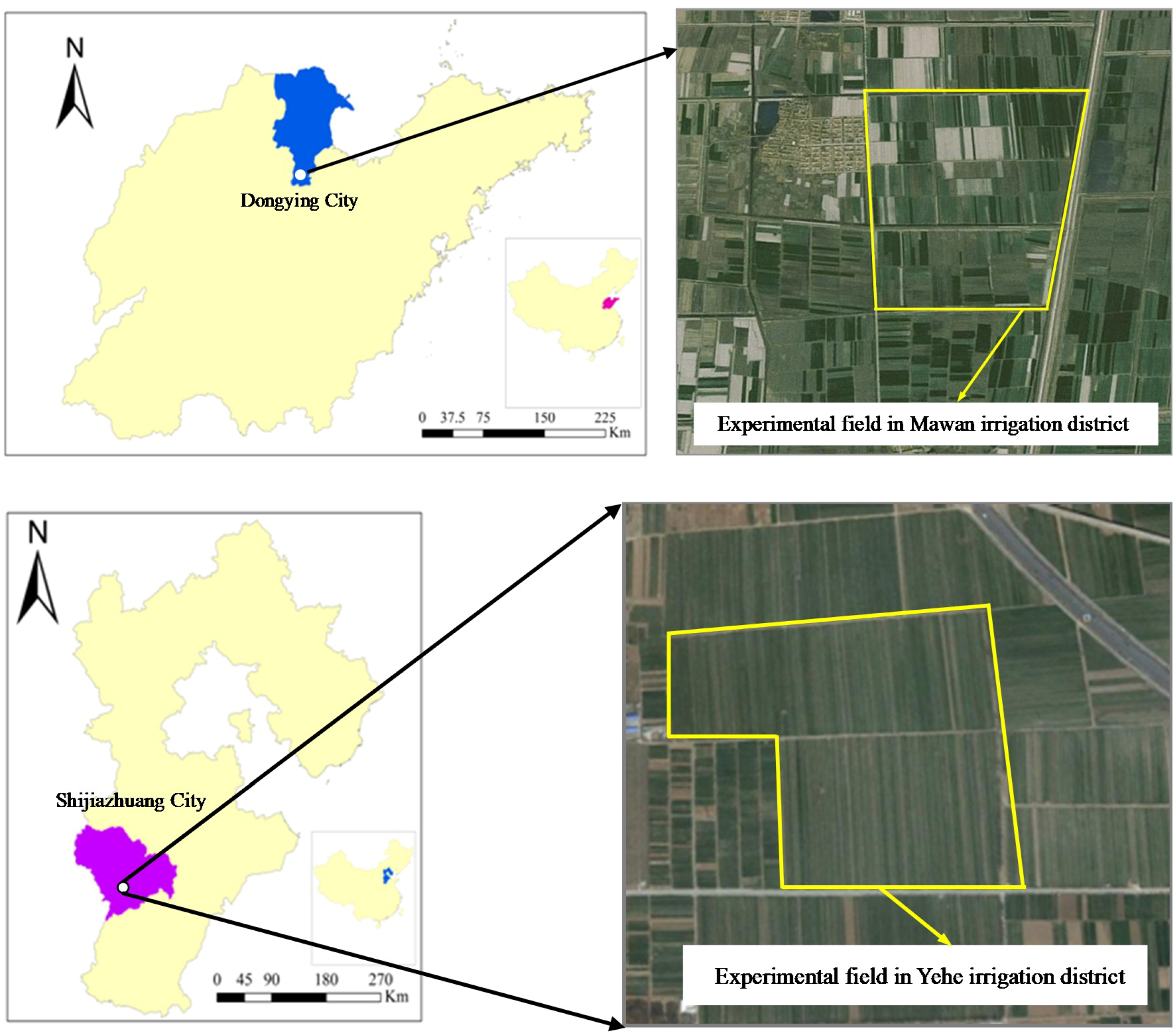
The first field experiment was conducted in the spring of 2012 at the Mawan irrigation district (MW) in Dongying City, Shandong Province, China and the second field experiment was conducted in the fall of 2012 at the Yehe irrigation district (YH) located in Shijiazhuang City, Hebei Province, China, as shown in Figure 1. The experimental field areas are 76.2 ha² in MW and 43.4 ha² in YH, respectively. MW is located in the coastal area of the lower reaches of the Yellow River, which has a typical warm temperate zone continental monsoon climate, with an average annual rainfall of 537.4 mm. The soils are alluvial sediments with primary textures of silt loam and sandy loam. YH is located in the North China Plain, which has a typical temperate zone monsoon climate, with the average annual rainfall of 444.1 mm. The experimental soil is classified as sandy loam in the root zone.

2.1.2. Data Collection

The border fields with 272 plots in MW and 154 plots in YH were used to irrigate the winter wheat by the Yellow River water and Gangnan reservoir water, respectively. Before the beginning of border irrigation, soil samples were collected at four depths (0 cm to 20 cm, 20 cm to 40 cm, 40 cm to 70 cm, 70 cm to 100 cm) from the middle of border field with 100 plots selected randomly to analyze soil bulk density, soil particle size distribution, and initial soil water content. After the end of border irrigation with a period of 48 h, soil samples were collected at four depths (0 cm to 20 cm, 20 cm to 40 cm, 40 cm to 70 cm, 70 cm to 100 cm) from the top, middle, and bottom of the border fields, with 100 plots selected randomly to analyze soil water content.

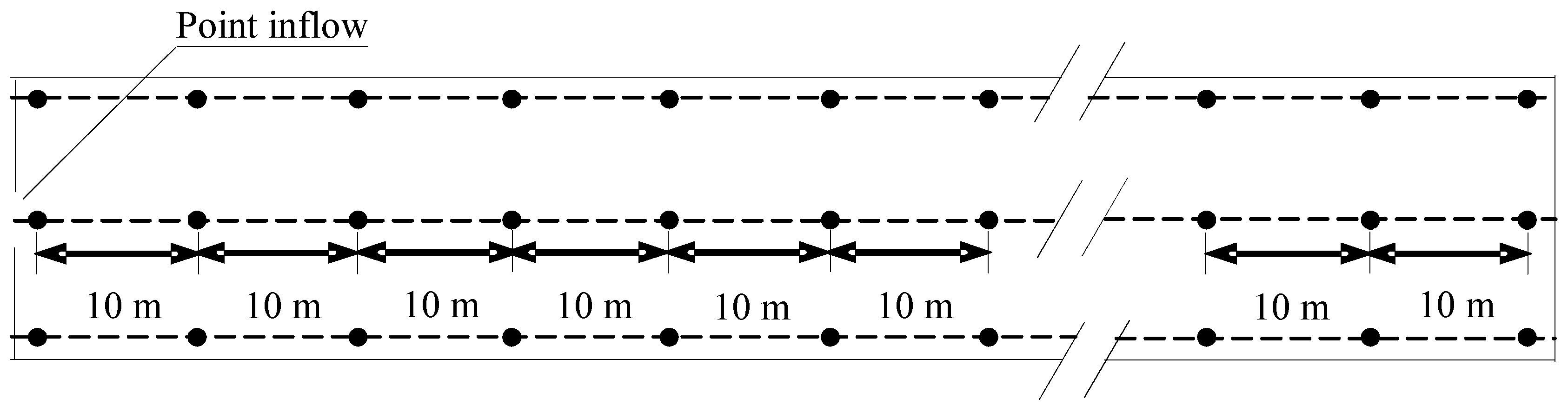
The relative surface elevation values of border field with 100 plots selected randomly were observed using a water level gauge, and the space between two adjacent measured points was 10 m for all experiments. Three lines were set at the left, middle, and right sides along the border width (Figure 2). The border length and width were measured using an engineering measure ruler. The observational tests for the surface flow advance processes were carried out at the beginning of surface irrigation (Figure 2). The surface flow depth was measured using water depth measuring devices [24], which were placed at every observation point before the irrigation was initiated. The water depth was used to estimate Manning’s roughness coefficient n [25]. The recorded data were then transferred to a computer at the end of the experiments.

2.1.3. Statistical Analysis of Field Physical Properties at a Field Scale

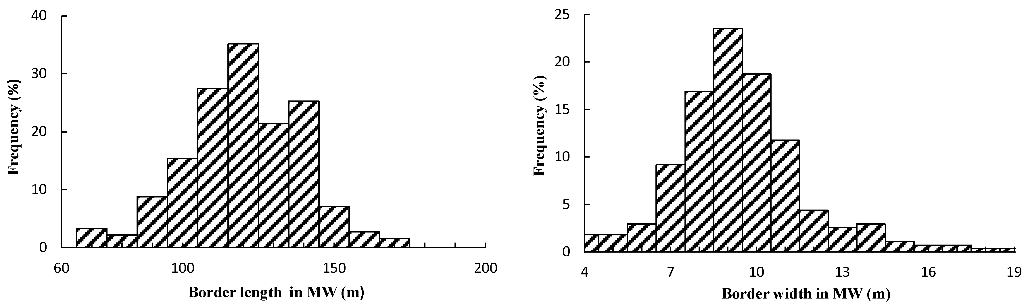
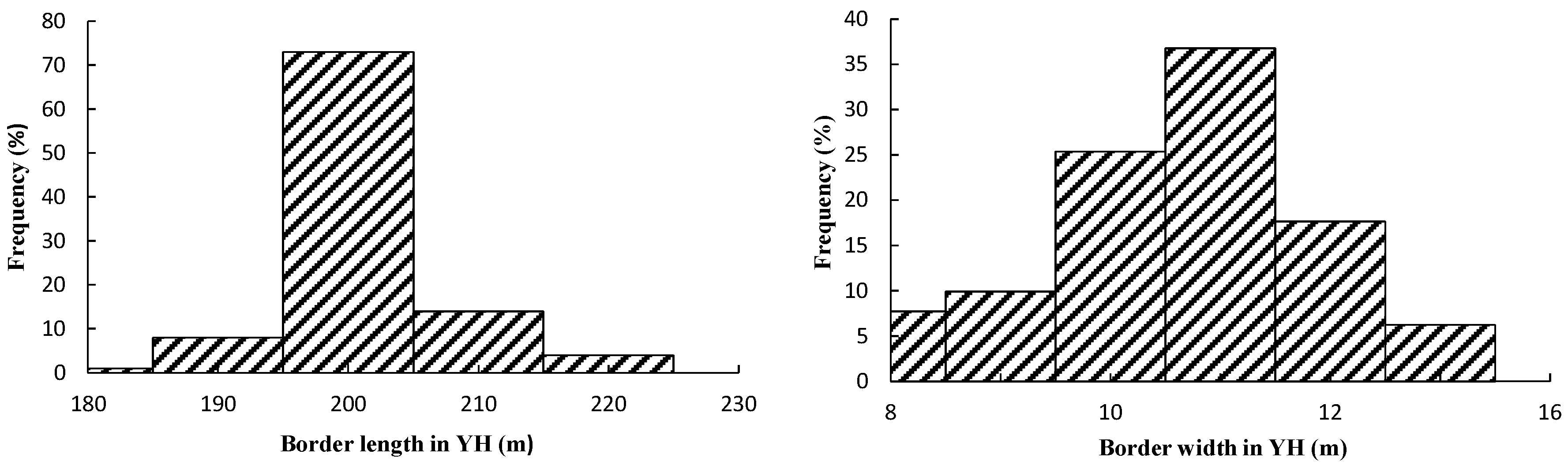
Border irrigation performance at a field scale is mainly affected by the spatial variability of field physical properties and field management measures. According to the same field tillage and management conditions, the frequency distribution histograms of border length in MW and YH are shown in Figure 3. It can be seen that border length in MW and YH presents the normal distribution characteristic and can be fitted by the normal distribution function. The mean values and standard deviations for the normal distribution of border length in MW and YH are 120, 33.6 m and 200, 30.2 m, respectively. Similarly, two parameters of the fitting distribution of border width in MW and YH are 9, 1.98 m and 6, 1.44 m, respectively.

The unit discharge is calculated on the basis of border width and inflow observed at the field experiments. The unit discharge presents the obvious statistical characteristics of normal distribution by the Kolomogorov–Smirnov test and the corresponding parameters and normal test results are shown in

Table 1. Statistical characteristics and normal test results of unit discharge of border field at a field scale.

Experiment Site	Minimum (L/(s·m))	Maximum (L/(s·m))	Mean (L/(s·m))	S.D.	K-S Test
MW	2.84	3.25	3.12	0.47	N
YH	3.03	3.53	3.30	0.56	N

N indicates normal distribution, K-S Test indicates Kolmogorov-Smirnov test, S.D. indicates Standard Deviation.

.

The same field tillage and management methods are conducted at a field scale. Therefore, the standard deviations of surface elevation differences from the fields of 100 plots are assumed as the same in this study. The surface elevation differences (SED) values are checked for normality by the Kolmogorov–Smirnov test and a normal distribution with a significance level of 0.05 is obtained. The mean values and coefficients of the standard deviation for the two experiments are 4.06, 0.12 cm and 3.5, 0.21 cm, respectively, calculated through the method of Bai et al. [26]. The spatial variability of the SED values is analyzed through the experimental semivariogram function, which can be fitted by the spherical semivariogram model [26]. The parameters of the spherical semivariogram model are calculated from the two sets of field-observed data (

Table 2. The parameter values of the pherical semivariogram model for surface relative elevation at a field scale.

Tests	The Pherical Semivariogram Parameters
	C0 (cm2)	C0 + C (cm2)	R (m)
MW	3.46	16.48	23.13
YH	3.31	15.76	37.53

MW indicates the Mawan irrigation district; YH indicates the Yehe irrigation district. C₀ indicates the nugget; (C₀ + C) indicates the still; R indicates the range.

). These parameters are used for the stochastic modeling of surface micro-topography. In addition, the field slopes in MW and YH are about 0.6‰ and 2.4‰, respectively.

The probability distribution characteristics of soil sandy loam, silt loam, clay loam, bulk density and organic carbon content can be obtained on the basis of the field-observed data. Each variable of soil properties in MW and YH is checked for normality by the Kolmogorov–Smirnov test. A log transformation is conducted if the statistical distribution of the raw data is highly skewed. The primary statistical parameters, such as the mean, maximum, minimum, and standard deviation values, are calculated. The statistical results of the soil properties, each variable of which represents the normal or log-normal distribution at a significance level of 0.05, are shown in

Table 3. Summary statistics of soil properties from the two experimental fields.

Tests	Indicators	Soil Properties
		SOC	Clay (<0.002 mm)	Silt (0.002–0.05 mm)	Sand (0.05–2 mm)	BD
		%	%	%	%	g cm−3
MW	Minimum	0.36	6.99	56.77	3.42	1.15
	Maximum	2.59	35.74	79.04	36.23	1.68
	Mean	1.13	19.91	65.97	14.12	1.38
	SD	0.42	5.18	4.22	4.66	0.36
	K-S test	N	N	N	N	N
YH	Minimum	0.75	9.17	18.47	15.38	1.14
	Maximum	1.78	33.87	61.38	64.89	1.62
	Mean	1.11	22.34	38.14	39.52	1.37
	S.D.	0.37	4.47	7.89	8.67	0.30
	K-S test	N	N	N	N	N

MW indicates the Mawan irrigation district; YH indicates the Yehe irrigation district. N indicates normal data distributions; SOC indicates soil organic carbon; BD indicates soil bulk density; S.D. indicates Standard Deviation; K-S test indicates Kolmogorov-Smirnov test.

.

According to the results of Agricultural Drought Research Center in the United States, the surface roughness coefficient can be determined by the crop growth situations and soil properties. The surface roughness coefficient values are checked for normality by the Kolmogorov–Smirnov test and a normal distribution with a significance level of 0.05 is obtained. The mean values and coefficients of the standard deviation for the two experiments are shown in

Table 4. Statistical characteristics and normal test results of surface roughness coefficient of border field at a field scale.

Experiment Site	Minimum (−)	Maximum (−)	Mean (−)	S.D.	K-S Test
MW	0.09	0.17	0.13	0.03	N
YH	0.08	0.14	0.10	0.02	N

MW indicates the Mawan irrigation district; YH indicates the Yehe irrigation district. N indicates normal distribution; S.D. indicates Standard Deviation; K-S Test indicates Kolmogorov-Smirnov test.

.

2.2. Numerical Modeling Methodology

Stochastic parameter model for surface irrigation is usually developed on the basis of deterministic irrigation model and stochastic parameter modeling method. In this section, we mainly introduce the physical-based surface irrigation model proposed by Dong et al. [23], which is a surface irrigation system model for the border irrigation simulation and implemented by coupling a one-dimensional surface flow model that uses the complete hydrodynamic form of the Saint-Venant equation with a one-dimensional subsurface flow model, and Monte Carlo simulation method, which is used to obtain the stochastic parameter values of the surface irrigation model.

2.2.1. Coupled Modeling of Surface-Subsurface Water Flow for Border Irrigation

Numerical simulation can be used to quantify surface irrigation application efficiency and surface irrigation distribution uniformity from irrigating fields and to design surface irrigation scheme based on controlling variables such as soils, border length, unit discharge, and surface micro-topography. In the proposed paper, the equations that govern the flow of water for surface irrigation modeling are presented below and the processes that describe water movement in the surface flow and subsurface flow domains are discussed.

Border irrigation water flow can be characterized by the complete hydrodynamic form of the one-dimensional Saint-Venant equations, which can accurately describe the non-steady water flow of surface irrigation. The continuity and momentum equations in the complete hydrodynamic model are taken as the governing equations:

$$\frac{\partial U}{\partial t}+\frac{\partial F}{\partial x}=S$$

(1)

where t is the time (s), x is the spatial coordinate (m), U is the vector of the conserved dependent variables, F is the physical flux, and S is the source vector that comprises bottom elevation vector S₁, bed roughness vector S₂ and infiltration vector S₃, which are expressed as:

$$U=\left(\begin{array}{c}{h}_s\\ q\end{array}\right), F=\left(\begin{array}{c}q\\ qu+\frac{1}{2}g{h}_s^2\end{array}\right), S=\left(\begin{array}{c}-I\\ -g{h}_s\frac{\partial z}{\partial x}-g\frac{n^{2}u\left|u\right|}{h_s^{1/3}}+\frac{u}{2}I\end{array}\right)$$

(2)

$$S_1=\left(\begin{array}{c}0\\ -g{h}_s\frac{\partial z}{\partial x}\end{array}\right), S_2=\left(\begin{array}{c}0\\ -g\frac{n^{2}u\left|u\right|}{h_s^{1/3}}\end{array}\right), S_3=\left(\begin{array}{c}-I\\ \frac{u}{2}I\end{array}\right)$$

(3)

where h_s is the water depth (m), q denotes the unit discharge along coordinate direction x (m³/s/m), g is the acceleration due to gravity (m/s²), z is the bottom elevation (m), n denotes the Manning’s roughness coefficient (m^1/6), and u is the vertically averaged flow velocity (m/s), I represents the infiltration rate (m/s).

Infiltration and soil water dynamics are simulated using the one-dimensional Richards equation, which describes vertical one-dimensional and non-hysteretic flow in a variably saturated porous medium

$$C(h)\frac{\partial h}{\partial t}=\frac{\partial }{\partial z}\left[K(h)\frac{\partial h}{\partial z}\right]-\frac{\partial K(h)}{\partial z}$$

(4)

where h is the pressure head (m), K(h) is the vertical hydraulic conductivity (m/min), C(h) = dθ/dh is the hydraulic capacity (−), z denotes the vertical coordinate(m), and t is the time (min).

The curve of soil water retention characteristics is described using the van Genuchten (1980) equations:

$$\theta (h)=\{\begin{array}{c}{\theta }_r+\frac{{\theta }_s-{\theta }_{{}^r}}{{(1+|\alpha h{|}^n)}^m} h<0\\ {\theta }_s h\ge 0\end{array}$$

(5)

and

$$K(h)=\{\begin{array}{c}{K}_s{S}_e^{1/2}{[1-{(1-S_e^{1/m})}^m]}^2 h<0\\ K_s h\ge 0\end{array}$$

(6)

where θ_s is the saturated soil water content (−), θ_r is the residual soil water content (−), α (1/m), n (−) and m (−) denote the soil water retention curve parameters, m = 1 − 1/n, and K_S is the saturated hydraulic conductivity (m/min), and S_e = (θ(h) − θ_r)/(θ_s − θ_r) is the effective saturation (−).

The hydraulic capacity is derived from van Genuchten’s model:

$$C(h)=\{\begin{array}{c}\alpha mn{\left|\alpha h\right|}^{n-1}{\left(1+{\left|\alpha h\right|}^n\right)}^{-\left(m+1\right)}\left({\theta }_s-{\theta }_r\right) h<0\\ 0 h\ge 0\end{array}$$

(7)

2.2.2. Numerical Solution

The various components of the mass and momentum conservation equations are solved by a hybrid numerical method to improve simulation accuracy and reduce computational effort. The details on the numerical solution of the complete hydrodynamic form of the one-dimensional Saint-Venant equations were previously discussed by Zhang et al. [20] and Dong et al. [23]; hence, only a brief description of it is provided.

At the time discretization used for the governing equations, the Crank-Nicolson implicit time scheme is used for $\partial \mathbf{U}/\partial t$, $\partial \mathbf{F}/\partial x$, and S₂ at an unknown time (w + 1) and a known time w. Then, S₁ and S₃ are discretized using the explicit time scheme at a known time w. At the space discretization of the governing equations, the finite difference scheme is used to discretize the space derivative of the physical flux linear approximation generated by the implicit time scheme. The advection upstream splitting method is used to discretize the space derivative of the advection physical flux, S₂ and S₃ are then calculated according to the corresponding space-node values. After spatio–temporal discretization processes of the governing equation of the one-dimensional complete hydrodynamic model, the discretization equations of mass conservation and momentum conservation are distinguished shown in Dong et al. [23]. The final format of surface flow equations can be expressed by:

$$BX=D\Rightarrow \left[\begin{array}{cc}{B}^{\mathrm{MA}}& 0\\ 0& B^{\mathrm{MO}}\end{array}\right]·\left\{\begin{array}{c}{X}^{\mathrm{MA}}\\ X^{\mathrm{MO}}\end{array}\right\}=\left\{\begin{array}{c}{D}^{\mathrm{MA}}\\ D^{\mathrm{MO}}\end{array}\right\}\Rightarrow \{\begin{array}{c}{B}^{\mathrm{MA}}{X}^{\mathrm{MA}}=D^{\mathrm{MA}}\\ B^{\mathrm{MO}}{X}^{\mathrm{MO}}=D^{\mathrm{MO}}\end{array}$$

(8)

where B is the coefficient matrix consisting of the coefficient of ΔU of cell (j − 1), j, (j + 1), respectively; at a known time w; B^MA is the coefficient matrix consisting of the coefficient of h_s of cell (j − 1), j, (j + 1), respectively, at a known time w; B^MO is the coefficient matrix consisting of the coefficient of u of cell (j − 1), j, (j + 1), respectively, at a known time w; X is the matrix of ΔU of each cell at a known time w; X^MA is the matrix of h_s of each cell; at a known time w; X^MO is the matrix of u of each cell at a known time w; D is the coefficient matrix of numerical flux vector of interface of cell j, bed roughness vector S₂, infiltration vector S_3, and the averaged form of bottom elevation vector S₁ of cell j at a known w; D^MA is the coefficient matrix about h_s and u at a known w; and D^MO is the coefficient matrix of numerical fluxes of interface of cell j, bed roughness, infiltration, and bottom elevation at a known w.

A finite volume method with fourth-order accuracy is used for the solution of the one-dimensional Richards equation in space, and the implicit second-order accurate finite difference scheme is used for the solution in time [23]. Then, the Picard iteration scheme [27] is applied to cope with the nonlinearity of the spatio-temporal discretization equation. Finally, the linearized algebraic equation obtained by spatio-temporal discretization processes is numerically solved. The discretized subsurface flow equation is as follows:

$$\begin{array}{l}C{(h)}_i^{k+1,m}\frac{3h_{{}^i}^{k+1.m+1}-3h_{{}^i}^{k+1,m}}{2\left(\mathsf{\Delta }t\right)}\mathsf{\Delta }{z}_i-F{(h)}^{k+1,m}·\left(h^{k+1,m+1}-h^{k+1,m}\right)\\ =-C{(h)}_i^{k+1,m}\frac{3h_i^{k+1,m}-4h_i^k+h_i^{k-1}}{2\left(\mathsf{\Delta }t\right)}+F{(h)}^{k+1,m}·h^{k+1,m}-K{(h)}_{i+1/2}^{k+1,m}+K{(h)}_{i-1/2}^{k+1,m}\\ \equiv R_p^{k+1,m}\end{array}$$

(9)

where $h_{{}^i}^{k+1,m}$ is the approximate value of the h of the ith cell at the mth discrete time level of the (k + 1)th time step, and R_P is the residual associated with the Picard iteration. If $R_{{}_P}^{k+1,m}\le {10}^{-5}$ and $\left|h_i^{k+1,m+1}-h_i^{k+1,m}\right|/h_i^{k+1,m}\le {10}^{-2}$, the iteration stops, the soil pressure heads of every spatial point at the (k + 1)th time step are calculated. The calculation then proceeds to the next time step.

For the surface flow system, the initial water depth h_s,initial and water flow velocity u_initial in each cell are zero before surface irrigation modeling is initiated. However, the numerical procedure requires all depths to be greater than zero to avoid undefined terms in Equation (1). Therefore, a small and positive value (0.0001 m) is initially assigned to the depth of flow at all cells in the flow domain. At the upstream end, the unit inflow rate is q = q₀. If irrigation stops, the water flow velocity at the field head is zero. The field end is closed. The initial time step for the subsurface flow system is given by users and the size of time step changes in accordance with the one used for the surface flow model. Time-variable surface pressure head h_s is set as the upper boundary condition; the bottom boundary conditions can be assumed as free drainage. The uniform pressure head throughout the soil profile is set as the initial condition in the computational domain.

This model can describe the impact of the interactions among soil, surface microtopography, field slope, roughness, border length and unit discharge on surface irrigation performance on a second time-step basis and exhibits the satisfactory simulation accuracy, low total volume balance error and high computational efficiency. Surface irrigation processes are described using the individual modules, which can be custom-configured to simulate soil water redistribution processes after surface irrigation. Further details on this model can be found in Dong et al. [23].

2.2.3. Monte Carlo Modeling

The proposed numerical methodology of modeling surface irrigation is also developed on the basis of stochastic parameter modeling method of controlling variables. In this section, Monte Carlo simulation method is used as the stochastic parameter simulation methodology.

Probability Distribution Functions of Model Parameters

Stochastic parameters, such as border length, unit discharge, soil hydraulic properties, surface micro- topography, field slope, and roughness, are input to the hybrid coupled model proposed by Dong et al. [23] as the initial conditions. Soil hydraulic properties are often nonlinearly related to soil sand content, clay content and organic carbon content. Therefore, soil hydraulic properties can be indirectly obtained from soil sand content, clay content, and organic carbon content using Pedo-Transfer Functions (PTFs). In order to assess border irrigation performance of field scale, the normal or logarithmic normal distribution functions are used to describe the distribution characteristics of controlling variables because of their spatial uncertainty. Border length, border width, unit discharge, soil sand content, soil clay content, and soil organic carbon content are of approximately normal distribution at a field scale. The probability distribution function of normal distribution can be expressed as follows:

$$f\left(x,u,\sigma \right)=\frac{1}{\sigma \sqrt{2\pi }}\exp \left(-\frac{1}{2}\frac{{\left(x-u\right)}^2}{{\sigma }^2}\right) u-3\sigma \le x\le u+3\sigma$$

(10)

where x is the controlling variable, u is the mean value of the controlling variable, and σ is the standard deviation of the controlling variable.

Surface micro-topography is one of the most important factors affecting the irrigation performance of a border irrigation system and it significantly affects the advance and recession processes of an irrigation event [28]. Micro-topography varies spatially along both the longitudinal and transversal directions of a border, thus the spatial distribution of surface elevation differences (SED) also affects the advance and recession processes and system performance. Therefore, the spatial variability of surface micro-topography includes the degree of unevenness of SED expressed by the standard deviation S_d and the spatial distribution of SED between the actual and the target design elevations. Under the same field tillage and management conditions, all of the S_d values of SED at a field scale are assumed as the same [26]. For a same S_d the spatial distribution of SED may vary, which makes it difficult to describe the impacts of the spatial variability of SED on surface irrigation performance. Therefore, surface micro-topography at a field scale can be represented by a set of elevation distributions of SED for the same S_d. Based on the field geometry (length and width) and the statistical characteristics of observed SED, the surface elevation nodes can be expressed by the following distribution:

$$f_{z_{\mathrm{mt}}}\left(z_{\mathrm{mt}}\right)=\frac{1}{\sqrt{2\pi }{\sigma }_{\mathrm{mt}}}\exp \left(-\frac{1}{2}\frac{{\left(z_{\mathrm{mt}}-u_{\mathrm{mt}}\right)}^2}{{\sigma }_{\mathrm{mt}}^2}\right) u_{\mathrm{mt}}-3{\sigma }_{\mathrm{mt}}\le z_{\mathrm{mt}}\le u_{\mathrm{mt}}+3{\sigma }_{\mathrm{mt}}$$

(11)

where z_mt is SED (cm), u_mt is the mean value of SED (cm), and σ_mt is the standard deviation of SED (cm).

Monte Carlo Simulation

Monte Carlo method is developed on the basis of probability and statistics theory and can be used to analyze most of the uncertainty issues. It is assumed that the probability distribution function of the random variable is known and a set of input parameter samples are obtained using the random sampling method. Thus, numerical models run based on the input parameter samples and output the corresponding simulation results. Finally, the performance indicators are calculated on the basis of the output data and their probability distribution characteristics are fitted, respectively.

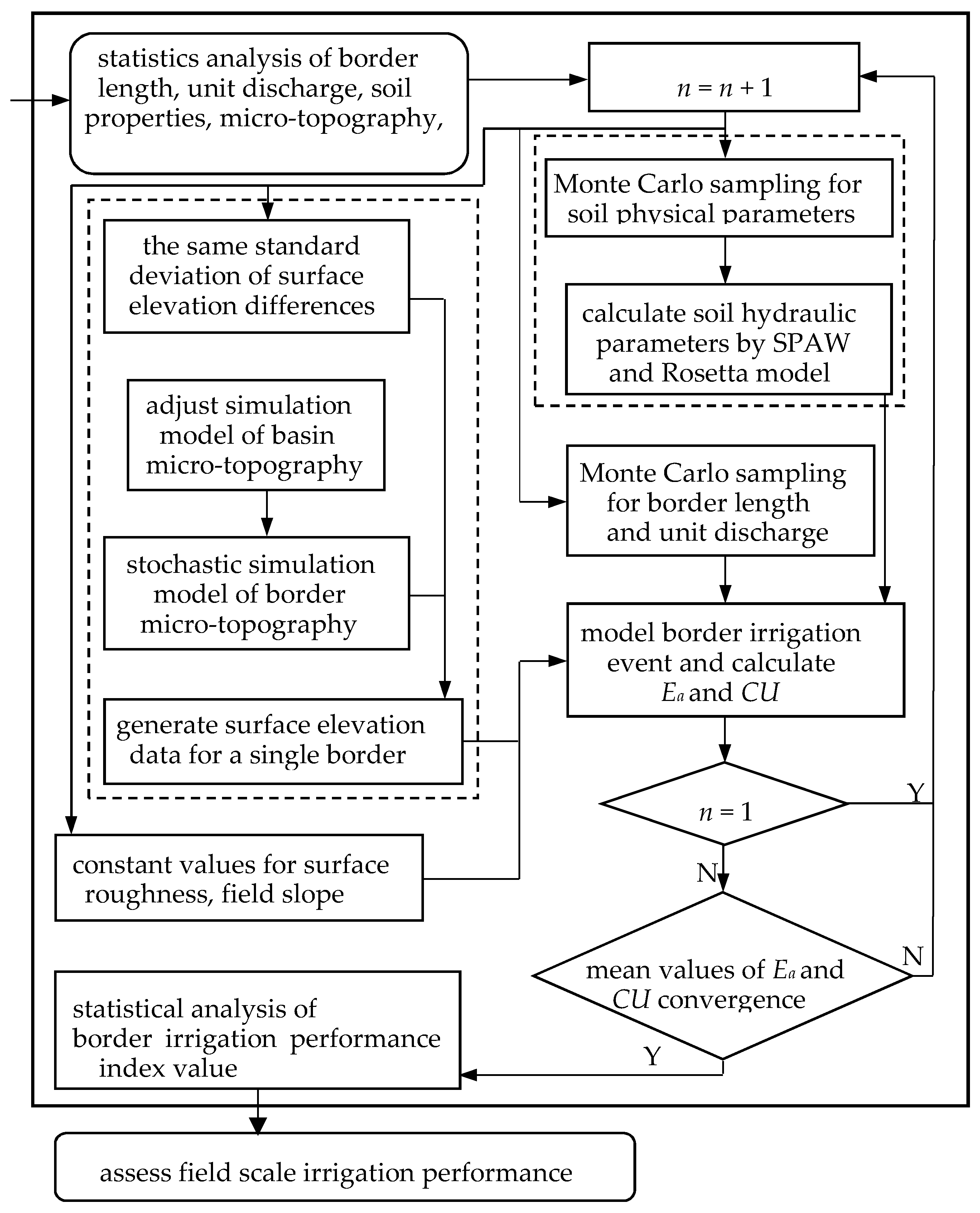
In the proposed paper, it is assumed that all of the border slope, surface roughness and the standard deviation S_d of surface micro-topography at a field scale are the same under the same filed tillage and management conditions and the spatial variability of soil properties, border length, unit discharge, and the spatial distribution of SED are the main factors that affect surface irrigation performance of field scale and the spatial distribution characteristics. The Monte Carlo simulation process of border irrigation at a field scale shown in Figure 4 is discussed as follows:

(1) The probability and statistical analysis of soil sand content, soil clay content, soil organic carbon, border length, unit discharge and SED are conducted on the basis of the field test data of field scale. The roughness coefficients of 100 plots selected randomly are calculated based on the surface elevation data and field slope values of 100 plots selected randomly are obtained based on surface water depth and crop growth situation.

(2) The probability distribution functions of soil sand content, clay content, silt content, and organic carbon content are obtained on the basis of the field test data of field scale and a set of random samples are obtained through their probability distribution functions by means of Monte Carlo simulation. If the parameter sample combinations of soil properties do not satisfy the given condition of Equation (12), the sample combination is replenished. Then, soil bulk density, field water holding capacity and wilt water content are obtained when the random samples of soil sand content, clay content and organic carbon content satisfying Equation (12) are input to Soil Plant Atmosphere Water (SPAW) software [29]. Finally, the random samples of soil sand content, soil clay content, soil organic carbon, soil bulk density, field water holding capacity and wilt water content are input to Rosetta software and the corresponding samples of soil hydraulic properties are obtained.

S_i + C + S + SOC = 100%

(12)

where S_i is soil silt content, %, C is soil clay content, %, S is soil sand content, %, and SOC is soil organic matter content, %.

(3) A set of border length and unit discharge samples are obtained through their probability distribution functions by means of Monte Carlo simulation, respectively.

(4) The number of surface elevation node in a single border is determined by field length, field width and the length of surface cell which is divided along the basin length direction. Surface elevation distribution data are generated by the stochastic simulation model of basin micro-topography, which is developed to simulate two-dimensional surface micro-topography on the basis of Monte Carlo method and Kriging interpolation method [26]. To simulate the one-dimensional border micro-topography, Equation (13) is used to update the above-mentioned surface elevation distribution data for border irrigation simulation:

$${\overline{z}}_{y,j}=\frac{1}{N_x}{\displaystyle \sum _{k=1}^{N_x}{z}_{x,k}} (j=1, 2, \dots , N_{\mathrm{y}})$$

(13)

where ${\overline{z}}_{y,j}$ is the average value of SED at the grid j along the basin length direction, representing the new SED value (cm), $z_{x,k}$ is the SED value at the grid k along the basin width direction (cm), N_x is the grid number along the basin width direction (−), and N_y is the grid number along the basin length direction (−).

(5) Steps (2) to (4) are repeated to obtain a set of random sample combinations, including border length, unit discharge, soil hydraulic properties, and surface micro-topography. These sample combinations and the constant parameters such as the mean values of field slope and roughness coefficient are input to the hybrid coupled model. Then, the hybrid coupled model runs repeatedly based on a set of stochastic parameter combinations and the border irrigation uniformity coefficient (CU) and border irrigation application efficiency (E_a) of each irrigation event are calculated based on the simulation values of soil water content along the border length direction. In the proposed paper, the maximum number of randomly selected samples is set to 272, which is the field-observed number.

(6) If the mean values of CU and E_a of the iteration (n + 1) and mean values of CU and E_a of the iteration n cannot satisfy the convergence criterion of Equations (14) and (15) (shown in Section 2.3), the iterative process continues. Otherwise, the iteration is terminated.

(7) The probability and statistical analysis method is used to analyze the changing trend of each evaluation indicator at a field scale, assess the impacts of spatial variability of field physical properties on border irrigation performance of field scale and optimize surface irrigation management plan at a field scale.

2.3. Evaluation Indicators of Surface Irrigation Performance

The application efficiency (E_a) and the uniformity coefficient (CU), as defined by Walker (1987), are selected as surface irrigation performance indicators. The application efficiency E_a (%) is defined as:

$$E_a=\frac{({\theta }_a-{\theta }_b)\times RD}{Z_{avg}}\times 100\%$$

(14)

and the uniformity coefficient CU (%) is given by:

$$CU=\left(1-\frac{{\displaystyle \sum _{i=1}^N\left|Z_i-Z_{avg}\right|}}{N\times Z_{avg}}\right)\times 100\%$$

(15)

where θ_a and θ_b are the average soil volumetric water content in the root zone before and after irrigation event, cm³/cm³, RD is the depth of root zone, cm, Z_avg is the average infiltrated depth of water applied to the field (mm) and determined from the cut-off time and the inflow rate, Z_i is the infiltrated depth of water in the ith field unit along the field length direction. N is the number of field units along the border length direction.

2.4. Model Performance Criteria of Field Scale

A numerical experiment is developed to assess the number of sets of generated stochastic parameter samples aiming at representing the spatial variability of field physical properties to be analyzed through simulation for assessing the impacts of the spatial variability of field physical properties on border irrigation performance at a field scale. Based on the probability distribution function of each variable of field physical properties, stochastic parameter samples are selected and input to the hybrid coupled model proposed by Dong et al. [23]. In these simulations with the hybrid coupled model, the same roughness, filed slope, and initial soil water content are used. When stochastic parameter samples are generated using the above-mentioned numerical methodology, more than one set of stochastic parameter sample can be generated. Different sets of stochastic parameter samples generated with the same condition will produce different values for the border irrigation performance at a field scale. Thus, it is necessary to determine how many stochastic parameter sample sets need to be generated for a given condition to appropriately analyze the impacts of the spatial variability of field physical properties on border irrigation performance at a field scale.

The number of stochastic parameter sample generations can be determined by analyzing the change trend of mean values of E_a and CU resulting from the simulation data of the different irrigation event through a set of stochastic parameter sample combinations. M sets of irrigation performance indicators can be obtained by modeling the different irrigation event with M sets of stochastic parameter samples for a given condition. The number m (m < M) of stochastic parameter sample generations required to characterize the spatial variability of field physical properties may be determined by analyzing the changes of border irrigation performance with the number of stochastic parameter samples generations. The irrigation performance simulation experiment is conducted through the hybrid coupled model. Statistical analysis is carried out by using Equations (16) and (17) (m < 272), which can reflect the effect of the stochastic parameter distribution on the border irrigation performance. If the MARE_k < 0.5% and RARE_k < 5% of six consecutive data points are used as the discriminant indicators that the mean value and standard deviation reach the steady state, the mean values of border irrigation performance indicators and the corresponding standard deviations can be determined. MARE_k and RARE_k can be calculated as follows:

$$MAR{E}_k=\left|\frac{{\overline{X}}_{k+1}-{\overline{X}}_k}{{\overline{X}}_k}\right|\times 100\%$$

(16)

$$RAR{E}_k=\left|\frac{S_d^{k+1}-S_d^k}{S_d^k}\right|\times 100\%$$

(17)

where MARE_k is the relative error between the (k + 1)th and the kth mean values of border irrigation performance indicators, RARE_k is the relative error between the (k + 1)th and the kth standard deviations of border irrigation performance indicators, $S_d^k$ represents the kth standard deviations of border irrigation performance indicators, and $S_d^{k+1}$ represents the (k + 1)th standard deviations of border irrigation performance indicators.

2.5. Data Analysis

The spatial variability of soil properties, border length, unit discharge and surface micro-topography results in the uncertainty of model input parameters. In order to represent the effects of the spatial variability of field physical properties on border irrigation performance at a field scale, the probability distribution and the classical statistical method are used in the proposed paper to verify the proposed stochastic model.

3. Results and Discussion

The proposed numerical methodology of assessing surface irrigation performance at a field scale is verified in this section.

3.1. Total Water Volume of Surface Irrigation

The total water volume of surface irrigation is defined as the sum of surface irrigation water volume applied to the experimental field at a field scale, calculated as,

$$V_s=\frac{A}{L\times W\times n}\times {\displaystyle \sum _{i=1}^n{V}_i}$$

(18)

where V_s is the total water volume of surface irrigation (m³), V_i is the irrigation water volume of the ith basin (m³), A is the total area of the experimental field (m²), L is the basin length (m), W is the basin width (m), and n is the number of basins in the experimental field (−).

The relative error of the total water volumes of surface irrigation between the simulation values and the observed values (RE_V) is calculated as,

$$R{E}_V=\frac{\left|V_s-V_o\right|}{V_o}\times 100\%$$

(19)

where V_s is the simulation value of the total water volume of surface irrigation (m³), V_o is the observed value of the total water volume of the surface irrigation (m³).

To assess the simulation performance of the proposed numerical methodology (PNM), the distributed numerical methodology (DNM) is employed. In distribution simulation, the experiment areas in MW and YH are divided into 16 and 12 sub-areas, respectively, according to soil properties, border length and unit discharge. The model parameters from each sub-area are input to the hybrid coupled model proposed by Dong et al. [23] and then the results of the sub-area level simulation are aggregated at a field scale to evaluate border irrigation performance in MW and YH, respectively. In the numerical modeling of the border irrigation, the considered surface spatial step along the border length is 2.5 m, and the considered subsurface spatial step along the vertical direction is 0.01 m. The time step of the surface and subsurface is 1 s. The initial soil water contents in MW and YH are 0.21 and 0.20 cm³ cm⁻³, respectively.

Table 5. The relative errors of the total water volumes from the model-predicted and the field-observed data.

Tests	Vo/m3	PNM		DNM
		Vs/m3	REV/%	Vs/m3	REV/%
MW	127,100	115,200	9.36	109,900	13.53
YH	72,300	65,900	8.85	62,300	13.83

MW indicates the Mawan irrigation district; YH indicates the Yehe irrigation district. PNM indicates proposed numerical methodology; DNM indicates distributed numerical methodology. V_o indicates the observed value of the total water volume of the surface irrigation; V_s indicates the simulation value of the total water volume of surface irrigation; RE_v indicates the relative error of the total water volumes of surface irrigation between the simulation values and the observed values.

presents the relative error of the total water volumes of the border irrigation between the model-predicted values and the field-observed values. The RE_V of the PNM is lower than that of the DNM. This result indicates that the PNM for scaling up the border irrigation performance at a field scale exhibits the more satisfactory simulation accuracy.

3.2. Surface Flow Advance

The surface flow advance time changes with the border length increasing and the maximum value appears at the bottom of the border. A power function curve such as described by Equation (19) is fitted successfully to the surface flow advance trajectories of the field-observed and the model-predicted, respectively.

$$T=a{X}^b$$

(20)

where T is the time of the surface flow advance (min), X is the length of the surface flow advance (m), and a and b are fitting parameters. Parameter a represents the change range of the whole surface flow advance trajectories and parameter b reflects the change in the speed of the surface flow advance rate.

The change trend of the surface flow advance trajectories within the surface irrigation processes can be expressed through parameters a and b of Equation (20). The parameter values obtained from each experimental field are checked respectively for normality through the Kolmogorov–Smirnov test statistics. They yielded a normal distribution with a significance level of 0.05. The relative errors of the average a and b values from the model-predicted and field-observed data were respectively calculated as

$$R{E}_p=\frac{\left|P_s-P_o\right|}{P_o}\times 100\%$$

(21)

where RE_p is the relative error of the average p value from the model-predicted data and the field-observed data, p represents the fitting parameters a and b, and P_s and P_o are the average values of the fitting parameters from the field-observed data and the model-predicted data, respectively (−).

Table 6. The relative error of the fitting parameter values from the model-predicted and the field-observed data.

Tests	Parameters	Po	PNM		DNM
			Ps	REp (%)	Ps	REp (%)
MW	a	0.1054	0.1017	3.51	0.1145	8.63
	b	1.3324	1.2928	2.97	1.2484	6.30
YH	a	0.1826	0.1742	4.60	0.1982	8.54
	b	1.2137	1.1718	3.45	1.1287	7.01

MW indicates the Mawan irrigation district; YH indicates the Yehe irrigation district. PNM indicates proposed numerical methodology; DNM indicates distributed numerical methodology. RE_p indicates the relative error of the average fitting parameter value from the model-predicted data and the field-observed data; P_s and P_o are the average values of the fitting parameters from the field-observed data and the model-predicted data.

presents the relative error of the average a and b values calculated from the model-predicted values and field-observed values, showing that the PNM has the better simulation performance compared with the FNM and SNM.

3.3. The Irrigation Time of Surface Flow Advance

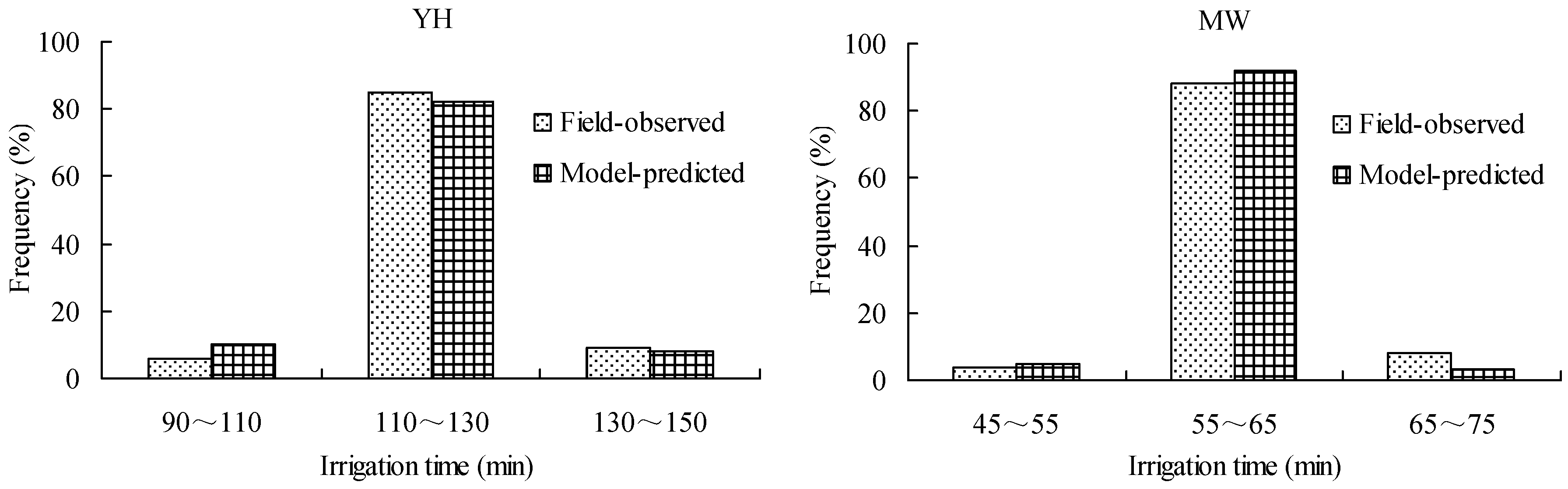
The irrigation time of surface flow advance (FT) is defined as the time of the surface flow arriving at the bottom of the border. The average absolute differences between the field-observed and the model-predicted values of the PNM and DNM are about 1.03 min, 1.46 min and 1.49 min, 2.1 min for the two experimental fields, respectively. The relative error of the average FT values of the field- observed and model-predicted data (RE_t) is calculated as,

$$R{E}_t=\frac{\left|t_s-t_o\right|}{t_o}\times 100\%$$

(22)

where t_s is the average FT value under the model-predicted conditions (min) and t_o is the average FT value under the field-observed conditions (min).

The statistical characteristics of the FT derived from the field-observed data and model-predicted data of the PNF for the two experimental fields are shown in Figure 5. The statistical characteristics of the FT from the field-observed data and model-predicted data of the PNM present the similar results, which indicate that the PNM performs satisfactorily. The relative errors of the average FT values from the field-observed and model-predicted data of the PNM and DNM are shown in

Table 7. The relative error of the average irrigation time from the field-observed and the model-predicted data.

Tests	to (min)	PNM		DNM
		ts (min)	REt (%)	ts (min)	REt (%)
MW	62.70	57.12	8.90	54.21	13.54
YH	116.50	108.36	6.99	102.86	11.71

PNM indicates the proposed numerical methodology; DNM indicates the distributed numerical methodology; MW indicates the Mawan irrigation district; YH indicates the Yehe irrigation district. t_s indicates the average irrigation time under the model-predicted conditions; t_o indicates the average irrigation time under the field-observed conditions; RE_t indicates relative error of the average irrigation time of the field- observed and model-predicted data.

, which illustrates that the PNM has the better simulation accuracy compared with the DNM.

3.4. Soil Water Content

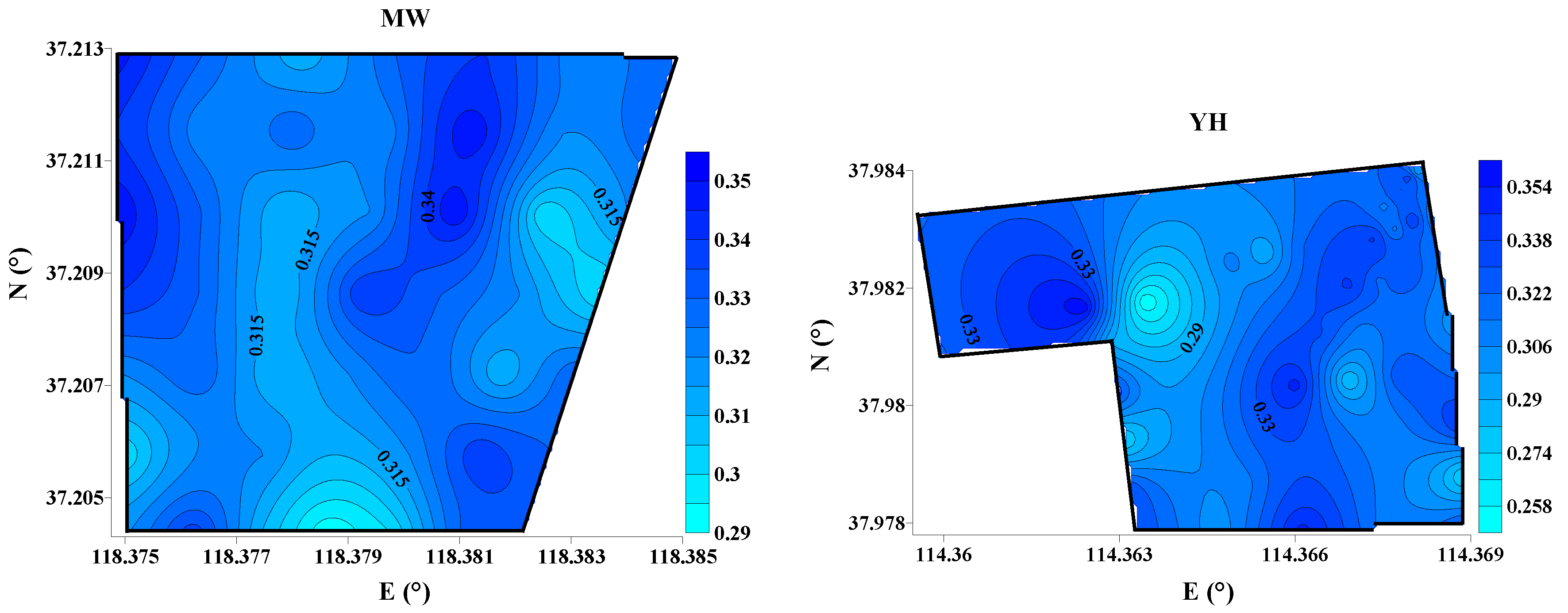
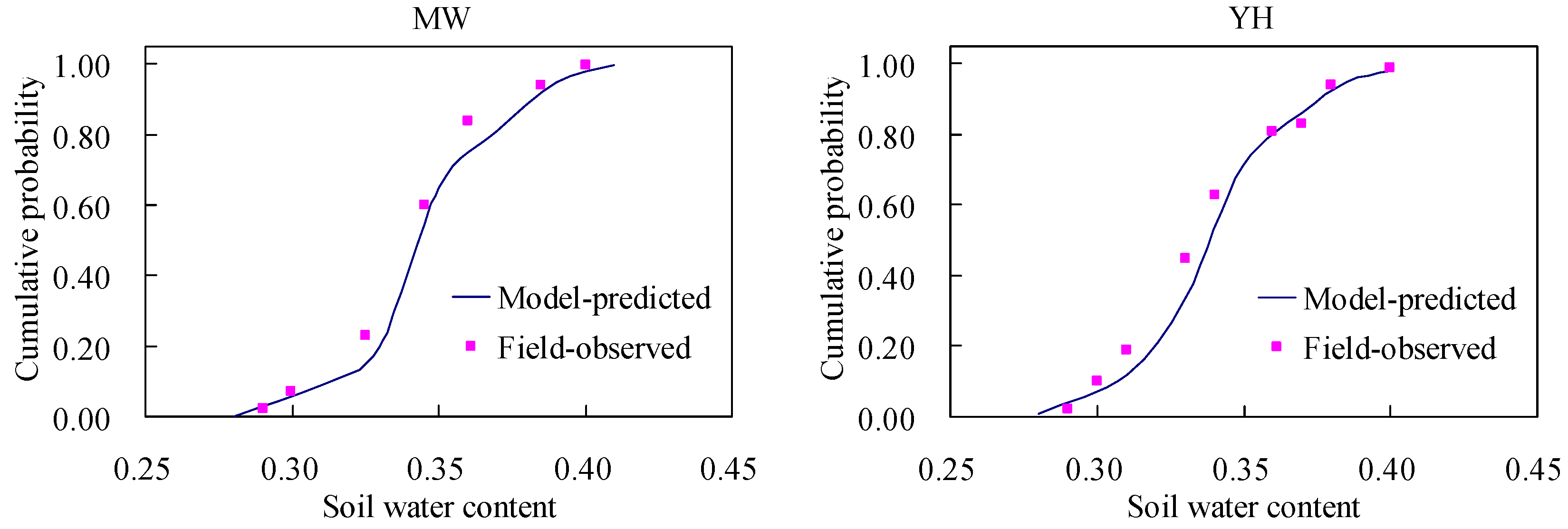
In this case, soil water content is used to assess the modeling accuracy of the proposed numerical methodology. The average soil water content of each sampling site is calculated based on those of three depths (0 cm to 20 cm, 20 cm to 40 cm, and 40 cm to 70 cm), using the weight average method. The spatial distribution of the average soil water content in MW and YH after the ending of the surface irrigation is intuitively presented in Figure 6. The spatial distribution data of the average soil water content were statistically analyzed to obtain the cumulative probability distribution of the average soil water content, as shown in Figure 6. The cumulative probability of the average soil water content of the model-predicted data with PNM, which is calculated using the soil water content data along the vertical direction of soil profile, is also shown in Figure 7. The agreement between the cumulative probability curves of the field-observed and the model-predicted data with the PNM is satisfactory.

4. Conclusions

To assess the impact of the spatial variability of field physical properties on the surface irrigation performance at a field scale, a numerical methodology is proposed on the basis of the hybrid coupled surface-subsurface flow model of surface irrigation and Monte Carlo simulation method. The hybrid coupled surface-subsurface flow model is developed from the numerical solution of the one-dimensional Saint-Venant equations using an improved hybrid numerical method and from the one-dimensional Richards equation using a finite volume method with fourth-order spatial accuracy. Monte Carlo simulation method is used to obtain the stochastic samples of field physical properties, and the stochastic simulation model of surface micro-topography is used to obtain a set of surface micro-topography samples for the same standard deviation of surface elevation differences. The proposed numerical methodology is tested in terms of the total water volumes of the surface irrigation, surface flow advance trajectories, irrigation time of each border, and soil water contents from the model-predicted and the field-observed data. Compared with the distributed-parameter modeling methodology, the proposed numerical methodology shows the better simulation performance in total water volume of surface irrigation, surface flow advance trajectories and soil water content redistribution. In conclusion, the proposed numerical methodology presents the satisfactory simulation performance and can be used as a tool for analyzing surface irrigation performance and similar hydrologic patterns at large scales.

References

- Strelkoff, T. One-dimensional equations of open channel flow. J. Hydraul. Div. 1969, 95, 861–876. [Google Scholar]
- Banti, M.; Zissis, T.; Anastasiadou-Partheniou, E. Furrow irrigation advance simulation using a surface–subsurface Interaction model. J. Irrig. Drain. Eng. 2011, 137, 304–314. [Google Scholar] [CrossRef]
- Kostiakov, A.N. On the dynamics of the coefficients of water percolation in soils and on the necessity of studying it from a dynamic point of view for purpose of amelioration. Int. Soc. Soil Sci. 1932, 1, 17–21. [Google Scholar]
- Elliott, R.L.; Walker, W.R.; Skogerboe, G.V. Zero-inertia modeling of furrow irrigation advance. J. Irrig. Drain. Div. 1982, 108, 179–195. [Google Scholar]
- Zerihun, D.; Furman, A.; Warrick, A.W. Coupled surface-subsurface flow model for improved basin irrigation management. J. Irrig. Drain. Eng. 2005, 131, 111–128. [Google Scholar] [CrossRef]
- Bautista, E.; Zerihun, D.; Clemmens, A.J. External iterative coupling strategy for surface-subsurface flow calculations in surface irrigation. J. Irrig. Drain. Eng. 2010, 136, 692–703. [Google Scholar] [CrossRef]
- Zhu, Y.; Shi, L.S.; Yang, J.Z.; Wu, J.W.; Mao, D.Q. Coupling methodology and application of a fully integrated model for contaminant transport in the subsurface system. J. Hydrol. 2013, 501, 56–72. [Google Scholar] [CrossRef]
- Tuli, A.; Kosugi, K.; Hopmans, J.W. Simultaneous scaling of soil water retention and unsaturated hydraulic conductivity functions assuming lognormal pore-size distribution. Adv. Water Resour. 2001, 24, 677–688. [Google Scholar] [CrossRef]
- Schaap, M.G.; Leij, F.J. Database related accuracy and uncertainty of pedotransfer functions. Soil Sci. 1998, 163, 765–779. [Google Scholar] [CrossRef]
- Skonard, C.J. A Field-Scale Furrow Irrigation Model. Ph.D. Thesis, University of Nebraska, Lincoln, NE, USA, 2002. [Google Scholar]
- Saxton, K.E.; Rawls, W.J. Soil water characteristic estimates by texture and organic matter for hydrologic solutions. Soil. Sci. Soc. Am. J. 2006, 70, 1569–1578. [Google Scholar] [CrossRef]
- Li, Y.; Chen, D.; White, R.E.; Zhu, A.; Zhang, J. Eatimating soil hydraulic properties of Fengqiu Country soils in the North China Plain using pedo-transfer functions. Geoderma 2007, 138, 261–271. [Google Scholar] [CrossRef]
- Wang, Y.Q.; Shao, M.A.; Liu, Z.P. Pedotransfer functions for predicting soil hydraulic properties of the Chinese Loess Plateau. Soil. Sci. 2012, 177, 424–432. [Google Scholar] [CrossRef]
- Awan, U.K.; Tischbein, B.; Martius, C. Combining hydrological modeling and GIS approaches to determine the spatial distribution of groundwater recharge in an arid irrigation scheme. Irrig. Sci. 2013, 31, 793–806. [Google Scholar] [CrossRef]
- Singh, R.; Kroes, J.G.; van Dam, J.C. Distributed ecohydrological modeling to evaluate the performance of irrigation system in Sirsa district, India I: Current water management and its productivity. J. Hydrol. 2006, 329, 692–713. [Google Scholar] [CrossRef]
- Paydar, Z.; Gallant, J. A catchment framework for 1-D models introducing FLUSH and its application. Hydrol. Process. 2008, 22, 2094–2104. [Google Scholar] [CrossRef]
- Todorovic, M.; Steduto, P. A GIS for irrigation management. Phys. Chem. Earth 2003, 28, 163–174. [Google Scholar] [CrossRef]
- Ahmadzadeh, H.; Morida, S.; Delavara, M.; Srinivasan, R. Using the SWAT model to assess the impacts of changing irrigation from surface to pressurized systems on water productivity and water saving in the Zarrineh Rud catchment. Agric. Water. Manag. 2016, 175, 15–28. [Google Scholar] [CrossRef]
- Anwar, A.A.; Ahnad, W.; Bhatti, M.T.; Haq, Z.U. The potential of precision surface irrigation in the Indus Bsain Irrigation System. Irrig. Sci. 2016, 34, 379–396. [Google Scholar] [CrossRef]
- Zhang, X.; Ren, L.; Kong, X. Estimating spatiotemporal variability and sustainability of shallow groundwater in a well-irrigated plain of the Haihe River basin using SWAT model. J. Hydrol. 2016, 541, 1221–1240. [Google Scholar] [CrossRef]
- Chen, B.; Ouyang, Z.; Sun, Z.; Wu, L.; Li, F. Evaluation on the potential of improving border irrigation performance through border dimensions optimization: A case study on the irrigation districts along the lower Yellow River. Irrig. Sci. 2013, 31, 715–728. [Google Scholar] [CrossRef]
- Fitzhugh, T.W.; Mackay, D.S. Impacts of input parameter spatial aggregation on an agricultural non-point source pollution model. J. Hydrol. 2000, 236, 35–53. [Google Scholar] [CrossRef]
- Dong, Q.G.; Xu, D.; Zhang, S.H.; Bai, M.J.; Li, Y.N. A hybrid coupled model of surface and subsurface flow for surface irrigation. J. Hydrol. 2013, 500, 62–74. [Google Scholar] [CrossRef]
- Li, Y.N.; Xu, D.; Li, F.X. Development and performance measurement of water depth measuring device applied for surface irrigation. Trans. CSAE 2006, 22, 32–36. (In Chinese) [Google Scholar]
- Xu, D.; Cai, L.G.; Wang, S.L. Farmland Water and Soil Management of Agriculture Sustainable Development; China Water Power Press: Beijing, China, 2000. (In Chinese) [Google Scholar]
- Bai, M.J.; Xu, D.; Li, Y.N.; Pereira, L.S. Stochastic modeling of basins microtopography: Analysis of spatial variability and model testing. Irrig. Sci. 2010, 28, 157–172. [Google Scholar] [CrossRef]
- Celia, M.A.; Bouloutas, E.T. A general mass-conservative numerical solution for the unsaturated flow equation. Water Rsour. Res. 1990, 26, 1483–1496. [Google Scholar] [CrossRef]
- Walker, W.R.; Skogerboe, G.V. Surface Irrigation Theory and Practice; Prentice-Hall, Inc.: Englewood Cliffs, NJ, USA, 1987. [Google Scholar]
- Keller, T.; Håkansson, I. Estimation of reference bulk density from soil particle size distribution and soil organic matter content. Geoderma 2010, 154, 398–406. [Google Scholar] [CrossRef]
Figure 1.
Location of the experimental fields in the Mawan and Yehe irrigation districts.
Figure 2.
The observed sites of the surface flow advance.
Figure 3.
The frequency distribution of border length and width at the Mawan and Yehe irrigation districts. MW indicates the Mawan irrigation district; YH indicates the Yehe irrigation district.
Figure 4.
Monte Carlo simulation processes of border irrigation at a field scale. Ea indicates application efficiency; CU indicates the uniformity coefficient; SPAW indicates Soil Plant Atmosphere Water model.
Figure 5.
The statistical distribution of the irrigation time of surface flow advance.
Figure 6.
The spatial distribution of the average soil water content of the field-observed after the ending of surface irrigation. MW indicates the Mawan irrigation district; YH indicates the Yehe irrigation district.
Figure 7.
The cumulative probability of the average soil water content for the field-observed and the model-predicted data with the PNM. MW indicates the Mawan irrigation district; YH indicates the Yehe irrigation district.