Improved Building Treatment Approach for Urban Inundation Modeling: A Case Study in Wuhan, China


1
School of Information and Safety Engineering, Zhongnan University of Economics and Law, Wuhan 430073, China
2
School of Accounting, Zhongnan University of Economics and Law, Wuhan 430073, China
3
Power China Hubei Electric Engineering Corporation, Wuhan 430040, China
*
Author to whom correspondence should be addressed.
Water 2018, 10(12), 1760; https://doi.org/10.3390/w10121760
Submission received: 15 August 2018
/
Revised: 19 November 2018
/
Accepted: 28 November 2018
/
Published: 30 November 2018
(This article belongs to the Section Urban Water Management)
Abstract
:This paper describes an improved building treatment approach (IBTA) for use in urban inundation modeling. In this approach, the ground surface elevation was raised by the threshold (h) of the building entrance height to account for both the blockage and storage effect of areas with dense building coverage. A higher roughness coefficient was assigned to the areas where buildings were located to compensate for the resistance effects caused by the inner wall of the structure. The campus of Huazhong University of Science and Technology (HUST) in Wuhan City, China, was used as a case study. Comparison between IBTA and several traditional building treatment approaches suggested that the model results were sensitive to the building treatment method and the threshold used for terrain preprocessing in dense building regions. Furthermore, as the interaction between the surface water flow and dense buildings were adequately represented by using a new terrain preprocessing approach, the proposed IBTA provided better performance in terms of maximum inundation depth and the peak depth time than the traditional approaches in areas with dense building coverage, such as that of the campus.
1. Introduction
With the acceleration of urbanization, urban flood events are increasing both in frequency and severity as a consequence of several factors, including reduced infiltration capacities [1] and wetland loss due to continued human activity in a watershed [2,3]. In recent years, urban inundation modeling has become increasingly important and has been identified as a research priority as demands for urban flood forecasting and risk assessment increase [4,5,6,7]. Estimates of flood damage for insurance and flood defense design, as well as flood risk management, are reliant on accurate predictions of water depth, extent, and duration provided by the urban inundation modeling [8,9,10]. In recent decades, a variety of inundation models have been reported and applied to river inundation estimations (including the adjacent floodplain) [11,12]. However, urban inundation is becoming less predictable and more uncertain due to the complex interaction between sewer and overland flow and hydrological variations driven by the spatial variability of surface elements [13,14]. Therefore, there is a need to develop computationally efficient and reliable urban flood models for risk analysis, damage assessments, and decision-making for urban flood prevention and control.
Many researchers have devoted their efforts to the development and application of methodologies for simulating urban floodplain inundation by means of numerical modeling. Since the flood inundation scenarios on a floodplain have a two-dimensional (2D) character, 2D distributed hydraulic models based on mathematical conservation laws for both mass and momentum have become justifiably popular. A number of studies have documented the application of 2D hydraulic models, such as TUFLOW [15], JFLOW [16], and LISFLOOD-FP [17]. These models, which mostly reveal the surface water flow by exploring 2D shallow water equations or their simplified variants, have been tested and verified with a range of boundary conditions and in various environments, and serve as an important tool to aid flood risk management [18,19,20]. However, the simulation approaches for urban inundation scenarios need to account for the topographic spatial heterogeneity and complex floodplain connectivity in urban areas, including the wave movement around the dense building areas.
In an urban environment, buildings will block the water flow and act as barriers in the flood inundation process [10,21]. Flood water flows around buildings, rather than into or through them, unless the water level rises above the crest heights of the entrances of the first building floor. As topography plays a major role in determining the flood wave propagation and water levels, the use of high-quality topographic data acquired from airborne or terrestrial LIDAR sensors can facilitate an improved representation of the flood flows around the small features in an urban area, such as buildings [22,23,24,25]. However, it will also require massive computational cost and complexity in the data preprocessing of urban topography, which leads to a tradeoff between model accuracy and efficiency [26,27]. In existing models, a bare-earth digital elevation model (DEM), in which the building features are removed, always serves as the base topography for 2D surface modeling applications in urban settings. Buildings are reinserted into the bare-earth DEM by different approaches based on their location to capture the local flow dynamics around buildings. The major building treatment methods used in these models are as follows:
Among these methods, the data preprocessing procedure of the BP method is the most complicated because the BCR and CRF for each DEM cell need to be evaluated before beginning the simulation. Therefore, the BP method is more appropriate for urban inundation modeling with coarser DEM grids [34]. Several studies have reported that the BR method is capable of accurately predicting highly irregular urban flood volumes [4,28], however such an increase in roughness often has no objective setting criteria to follow [35]. A more detailed discussion and comparison of these four methods in various conditions and environments is given by Schubert and Sanders [36]. The results demonstrate that all the building treatments mentioned above can reveal the blockage or drag effect caused by buildings. In practical terms, we can choose one of these methods based on the practical conditions, including available data, computing resources, time constraints, and the specific modeling objectives.
Although the abilities of these building treatment methods have already been validated in various field validation studies, there is little consideration of the internal storage capacity of buildings in most of them. Most of these methods are focused on the boundary conditions around the roof print of buildings (building outlines), and do not simulate the flood routing processes inside the buildings [10,37]. However, the area covered by buildings will become available for water storage when the water depth exceeds the crest height of the building entrance, in which case a considerable amount of water will be stored inside the building. Therefore, the rooms on the first floor of buildings are a non-negligible area for storing flood water, and they need to be addressed in urban inundation modeling.
A poor representation of building blockage and storage effects will affect the performance of an urban inundation model in terms of inundation extent, depth and speed of flow, which is significant for various flood-related risk analysis and loss assessments, including, in particular, impact analysis on critical infrastructure, traffic and personal safety [34]. It is, therefore, necessary to describe a new terrain preprocessing approach that can provide a better representation of both the blockage and storage effects caused by buildings in urban inundation models.
Consequently, the primary aim of this study is to explore and quantify the different simulation results when using varied building treatment approaches for urban inundation modeling, and to obtain a better understanding of model sensitivity to different building treatment methods, and to propose an improved building treatment method that is more comprehensive, objective, and practical. The rest of the paper is structured as follows: We first describe the details of the materials and methodology, including a presentation of the case study and inundation models. The proposed IBTA is then introduced to urban inundation models and tested against two real flood events that occurred in the study area. Then, the results are presented, and the comparison analysis between the IBTA and several traditional building treatment approaches is outlined. Finally, the major findings of this study are listed and conclusions are drawn.
2. Materials and Methods
2.1. Improved Building Treatment Approach (IBTA)
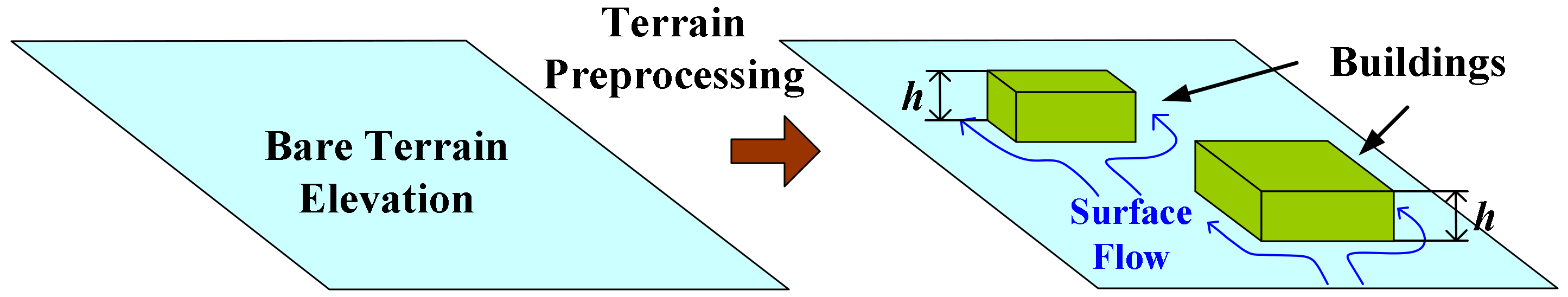
In urban inundation modeling, a geometric description represents the topography in the model through elevations defined on mesh grids, so we can raise the ground elevations where buildings are located to account for the obstructions in the flood wave propagation. However, the building elevation is set to the elevation of the roof in the BB method [29,30,31], so the flood water will never reach the interior areas of the buildings unless the water level reaches the roof height. The BH method, which treats building outlines as free slip walls, does not allow for flood water to reach the interior spaces of buildings [32,33]. For the BR method, on the other hand, as the shape of the building is not included in the domain topography, water can enter and flow through the buildings without any solid block. The BB (or BH) method and BR method can be understood to provide two extremes, either no water is allowed to enter the buildings or the buildings are totally filled with water. However, it is likely that the real circumstances would be somewhere in the middle of these two extremes, as buildings block the surface flow at first, and then become available for water storage when the flood level exceeds the building entrance height. In this sense, we expanded on the BB method to consider both the blockage effect and storage capacity of buildings by using alternative building elevation. In the IBTA, the ground elevations of DEM cells occupied by buildings were raised by the threshold (h) of the building entrance height (see Figure 1). Hence, the inner area of the building will be available for water storage when the water level exceeds the crest heights of the entrances of buildings. Although different buildings have different entrance heights, a fixed threshold for the entire study area is essential to reduce model complexity. In this study, two thresholds of building entrance height were set, 0.4 m and 0.6 m. For the IBTA0.4, buildings were assumed to be a constant 0.4 m above the local ground level elevation, which prevents water from flowing into the buildings until the water depth outside the buildings exceeds 0.4 m. For IBTA0.6, the surface elevation of the area covered by buildings was raised by 0.6 m, which prevented the flood water from entering the buildings when the water depth was below 0.6 m. The presence of inner walls, furniture, and closed doors may also decrease the flow rate and increase the surface resistance in buildings. After flowing into the building though the entrance, flood water is more likely to be inhibited by the buildings due to internal structural impedance. To account for this resistance effect acting on the flow inside buildings, we designed a variant of IBTA0.4 (IBTA0.4R) that combines IBTA0.4 with the BR method by assigning higher roughness values at the building’s position. These building treatment methods, including IBTA0.4, IBTA0.6, and IBTA0.4R, together with BH, BB, and BR, were all implemented within an urban inundation model, and the model sensitivity to different terrain processing approaches was evaluated and analyzed, as presented in Section 3.
2.2. Study Area
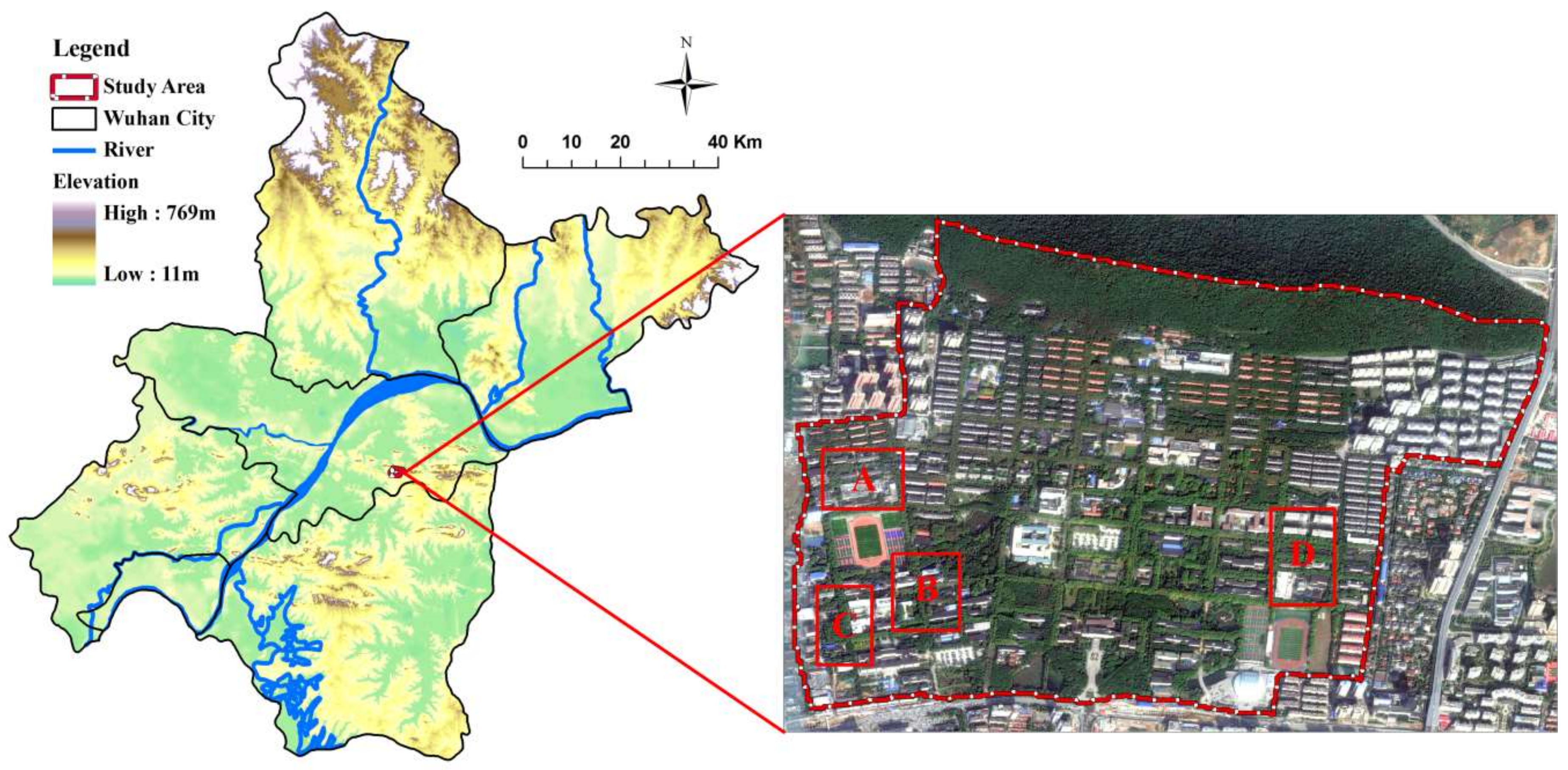
In this paper, the main campus of Huazhong University of Science and Technology (HUST) in Wuhan City, China, was selected as the study area. Wuhan City lies to the east of the Jianghan Plain, and the intersection of the middle reaches of the Yangtze and Han Rivers. Wuhan has a subtropical humid monsoon climate with a mean annual precipitation of 1269 mm over the last 30 years. The study area is situated in the southeast of Wuhan City and covers a total area of approximately 1.96 km2, with an elevation varying from 25 m to 141 m above sea level. As can be seen in the satellite image from Figure 2, the campus consists of a combination of track grounds, school buildings, and student apartment blocks within a topologically regular grid network of streets, and some open areas with forest cover and shrub cover in the southern and northern borders, and there is no significant water system that lies in or flows across the campus.
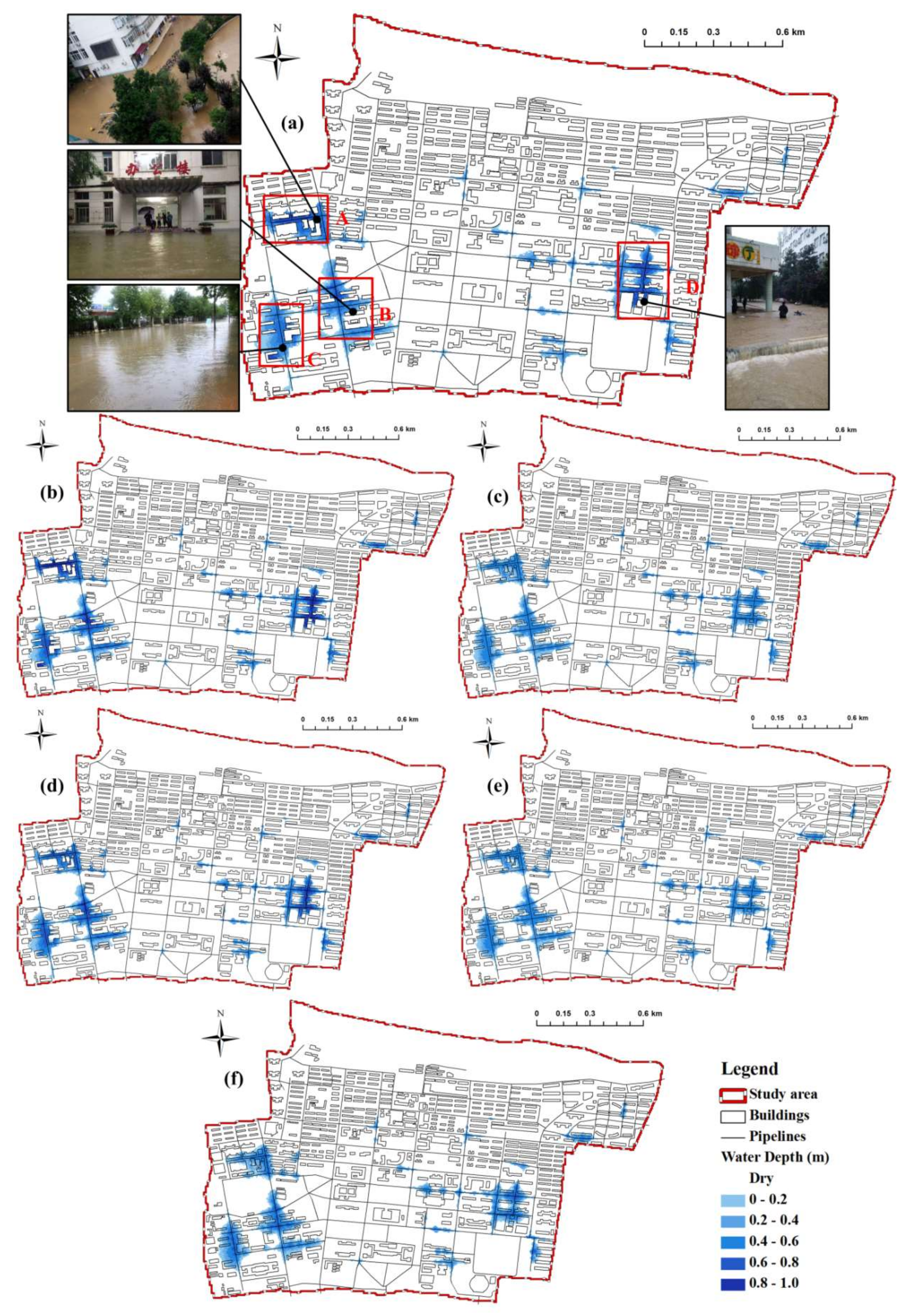
The study area has repeatedly experienced extreme floods and inundations due to the rainfall intensity in Wuhan and a poorly engineered flood control infrastructure. On 1 July 2016, Wuhan City was hit by the heaviest rainstorm since 1998 (76 mm of rainfall over a six hour period). The surface runoff volume caused by the storm exceeded the capacity of the drainage and pump systems, which eventually resulted in a serious flood inundation in the study area. However, aside from the maximum inundation depth at several control points, no flow measurements were available from this event. Therefore, the simulated flood extent was assessed against the approximate value gathered from eyewitness accounts and historical photography across the study area. Flooding was observed originating from the mid-eastern and southwestern parts of the campus, and the flood water subsequently flowed along Zisong Road, Nanyi Road and Hongmian Road, before finally pooling around the complex configuration of student apartment buildings located in the center and western side of the study area. The regions that were reportedly most at risk from the surface water flooding are highlighted in Figure 2 by red-bordered rectangles and are denoted as follows: A—Nanyi Road; B—Zisong Road; C—Laboratory of Coal Combustion; and D—Doctor Apartment. The simulation results for these regions will be analyzed and discussed in detail in Section 3. Consequently, it was important for us to apply the proposed IBTA to the campus and investigate the role of the building blockage and storage effect on flood wave propagation and inundation modeling in the urban floodplain.
2.3. Inundation Model
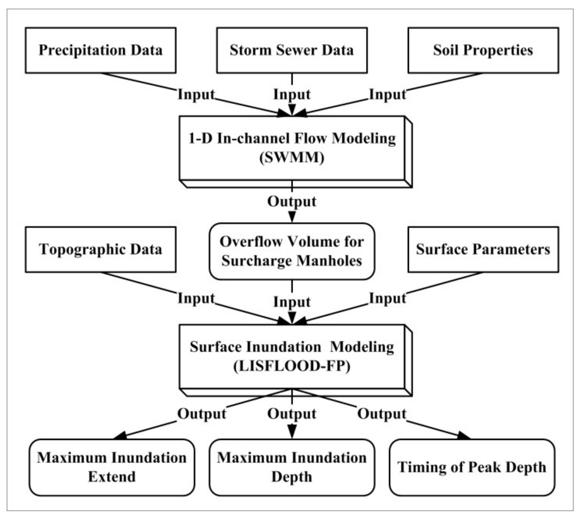
To simulate a flood inundation map for the study area, we introduced a coupled urban flood inundation model based on a 1D module in the SWMM model and a simplified 2D model in LISFLOOD, as shown in Figure 3.
Urban flood inundation is driven by the inability of storm sewer systems under ground to handle all the water from heavy rains [1,38]. Serving as the simulation method for the in-channel flow of the sewer system, the SWMM model was used in this study. SWMM is a dynamic rainfall runoff simulation model that can provide a reliable simulation of the water flow in a storm sewer system and the surcharged flow at manholes based on the 1D Saint-Venant equations [39,40,41]. The output of the SWMM, the time series of the overflow volume for each surcharge manhole, served as the input of the surface inundation modeling, which was performed using the LISFLOOD-FP model. The LISFLOOD-FP is a raster-based hydraulic model which was first developed by Bates and De Roo [17]. Since then, the model has undergone extensive improvements and testing [42,43]. In the LISFLOOD-FP, the floodplain flow is approximated as a 2D diffusion wave, and the fluxes of water between the floodplain elements are calculated using the continuity equation and Manning’s equation [17]. The LISFLOOD-FP provides good urban inundation predictions, including the inundation area, depth, and flow volume over complex topography represented by high-resolution DEMs. Moreover, the LISFLOOD-FP is an open source model, and its complexity has been reduced by neglecting less significant equation terms or improving the numerical schemes to speed up the solving procedures. These advantages have facilitated its widespread use in flood propagation modeling over large urban areas [20,44,45]. In this study, the simulation results of inundation area, depth and timing of the peak value were produced by LISFLOOD-FP.
2.4. Data Sources and Preprocessing
2.4.1. Precipitation Data
In this study, two flood events that occurred on 20 June 2016 and 1 July 2016 were used to calibrate and validate the model, respectively. According to the open hydro-meteorological database provided by the Meteorological Bureau of Hubei Province, the rainfall records of these two flood events are shown in Figure 4a,b. For the flood event of 20 June 2016, the total precipitation during the five hours of the storm was 55.6 mm, most of which (39.5 mm) fell in a 1.5 h period, between 11:30 and 13:00, accounting for approximately 71% of the total precipitation. The storm that occurred on 1 July 2016 was less concentrated, but even more intensive than the storm of 20 June 2016. Rainfall poured heavily from 7:45 to 9:15 and the peak rainfall intensity in this period reached 42.8 mm/h, within which rainfall amount (48.3 mm) accounted for over 63% of the total (76.8 mm) in the storm.
2.4.2. Topographic Data
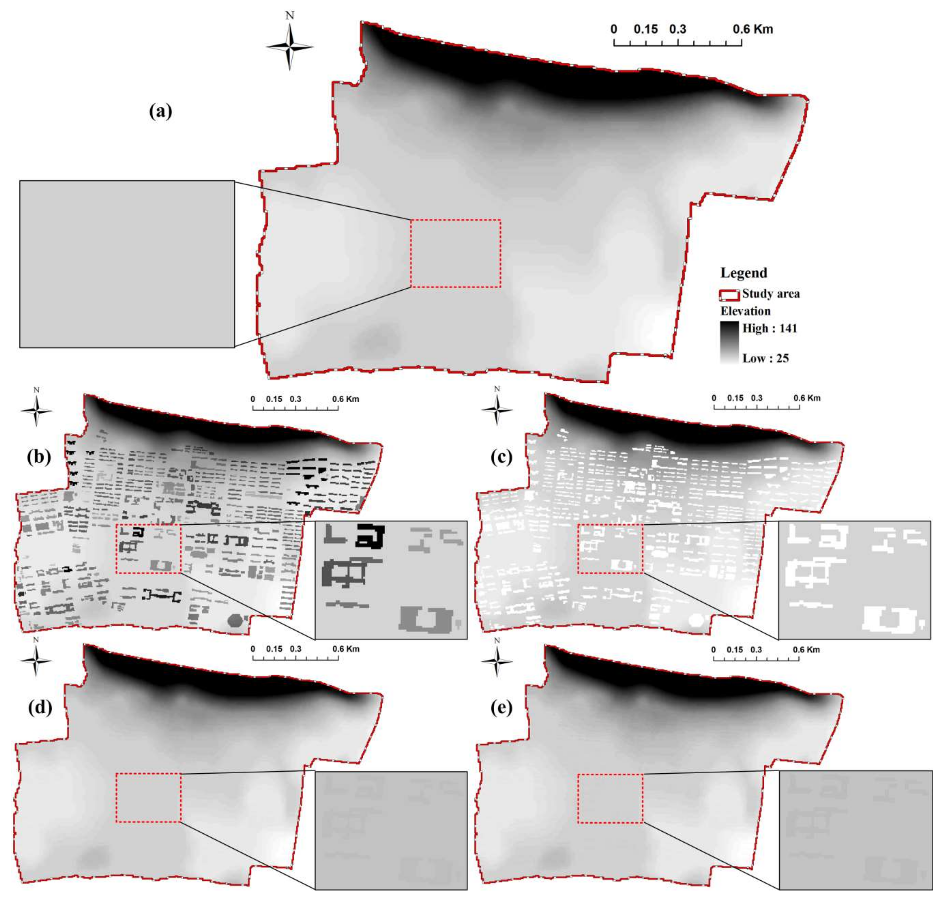
The topography of the study area was defined from a five-meter resolution gridded DEM consisting of 97,011 DEM cells, which was provided by Power China Hubei Electric Engineering Corporation (PCHEEC). The bare-earth DEM is shown in Figure 5a. The study area is characterized by a flat topography with hills in the north, and the surface elevation decreases slightly in the southeast and southwest.
2.4.3. Buildings Data
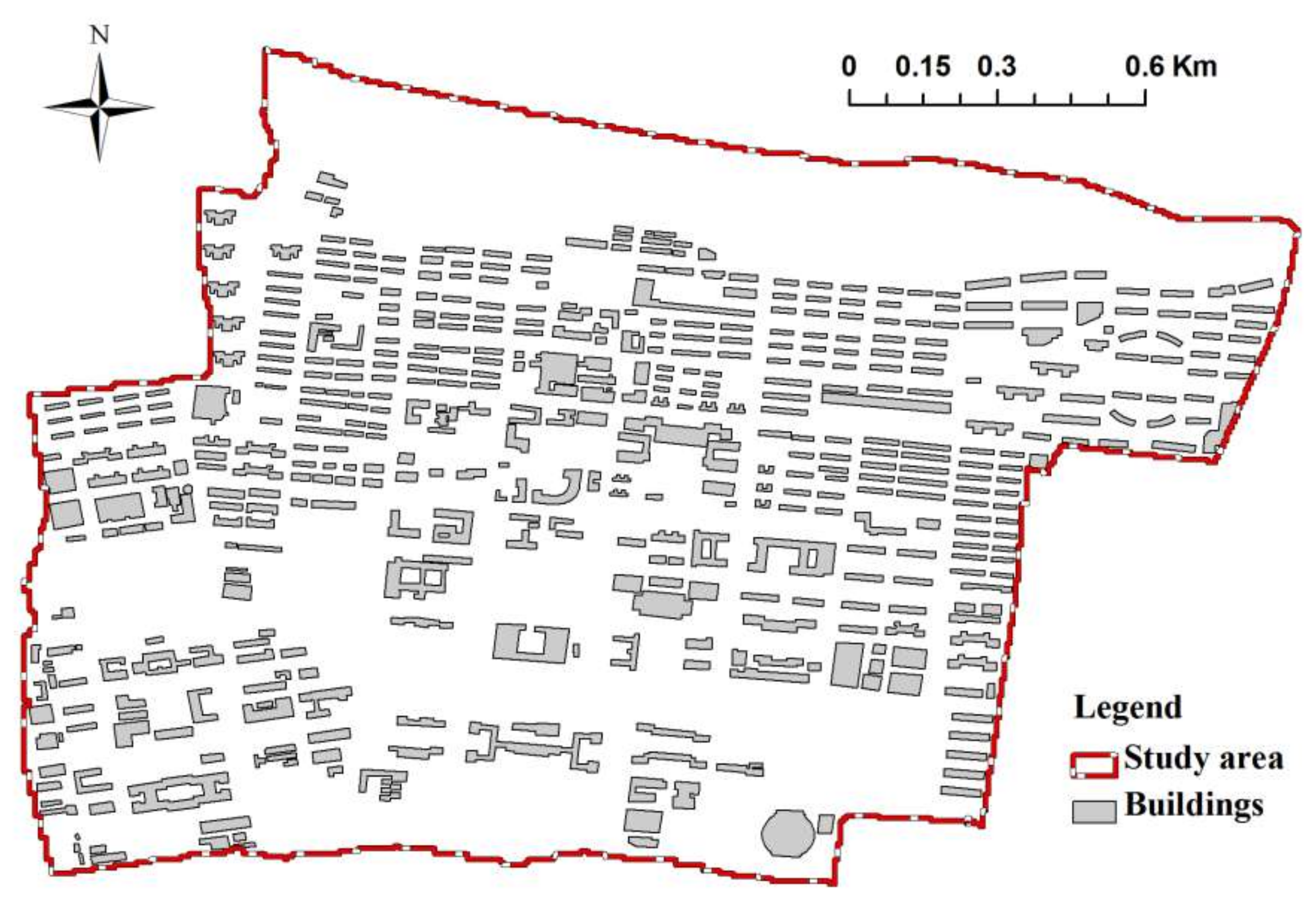
The geometry of the buildings was obtained from the Planning and Design Office of HUST. These were manually validated using the Google Street Map and were then organized as a polygon geometry layer in ArcGIS (Figure 6). There are approximately 498 buildings in the study area, which are densely distributed along the roads of the campus.
Figure 7a shows the building size distribution in the study area, which was created by approximating all buildings as rectangles and extracting the shortest dimensions. The separation distances between pairs of buildings were also computed, based on the building footprint outlines and the distribution, as shown in Figure 7a. A total of 98% of the buildings are five meters or larger, and 70% of the building separation distances fall in the range of 5 m to 15 m. Building sizes and gaps were calculated in this study since they both represent meshing constraints for the DEM data. A coarser grid may smear the flow path between a pair of buildings, which can convey surface water and consequently change the hydraulic behavior, thus resulting in inadequate predictions [34]. Therefore, grid resolutions below the length scales of building size and gaps were required to depict a flow path for every building treatment method considered in this study. Fewtrell et al. [10] highlight an initial estimate to the minimum DEM gird cell size for urban inundation modeling, which needs to be approximately equal to the length of the shortest building size or separation distance. Hence, it was adequate for this study to represent the topography of the study area and analyze the interaction between flood flows and buildings by using DEM grids with a five-meter resolution. Figure 7b provides the statistics on building entrance heights in the study area obtained from the measurements of 100 samples of buildings in the campus. It is noted that 84% of the building entrance heights in samples fall within the range of 0.3 m to 0.7 m. According to the histogram shown in Figure 7b, two values (0.4 m and 0.6 m) were chosen to reflect the threshold of building entrance height in this study.
2.4.4. Storm Sewer Data
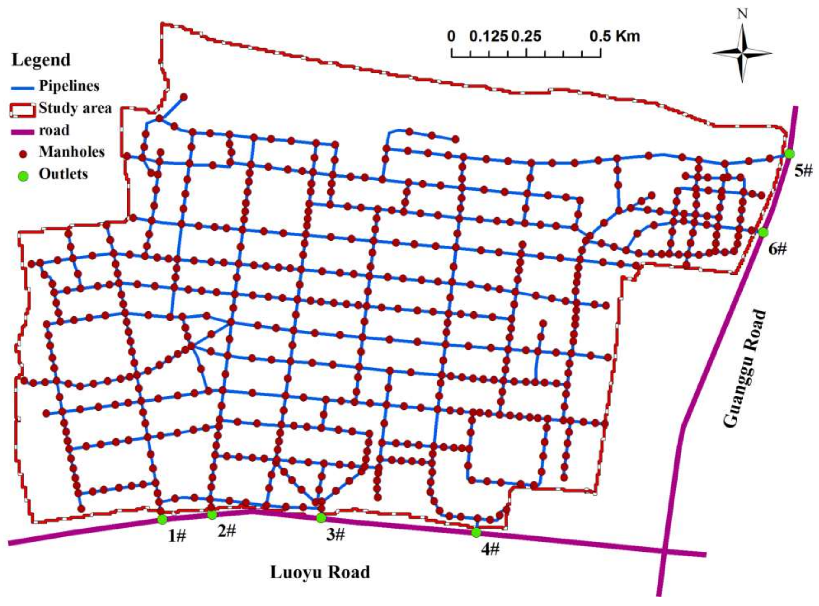
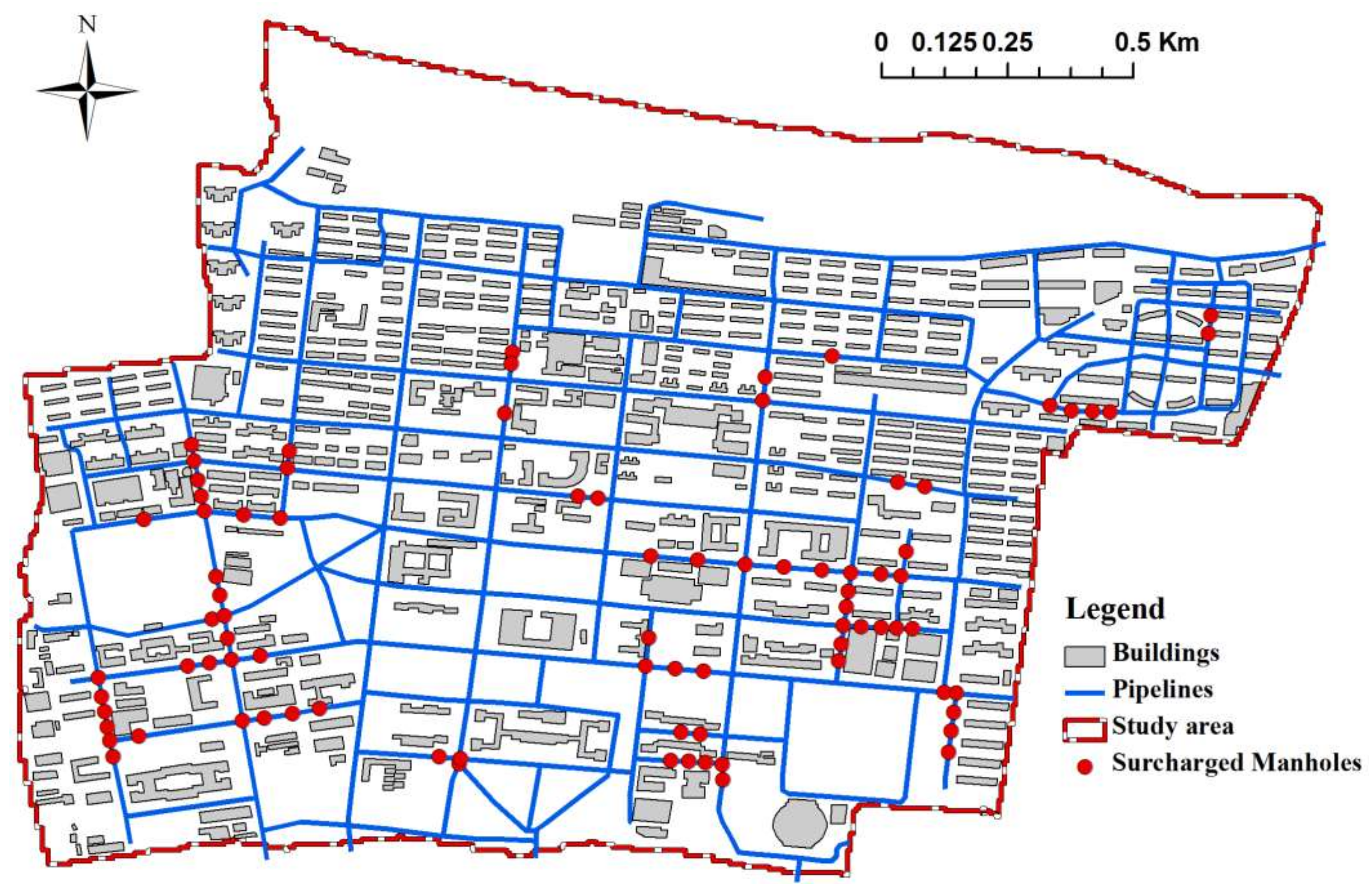
As no significant water system can be found on the satellite image, surface runoff in the study area appears to be mainly drained by the storm sewer system and to finally be discharged into the main sewer under Luoyu Road and Guanggu Road. Figure 8 describes the geospatial and geometric information of the storm sewer system in the study area, which was obtained from the Planning and Design Office of HUST. The storm sewer system consists of 54 pipelines, 617 manholes and six outlets numbered from #1 to #6, of which #1 to #4 are the outlets leading to Luoyu Road on the south side of the campus, and #5 and #6 are located under Guanggu Road on the east side.
2.4.5. Terrain Preprocessing
For building representation mean, the bare-earth DEM that is shown in Figure 5a was preprocessed based on the algorithms of the different building treatment methods, as follows:
- BB method: DEM cells that are occupied by buildings were raised by the roof height of the buildings. The result is shown in Figure 5b.
- BH method: Areas demarked as buildings in the bare-earth DEM were removed, and thus mesh holes were formed that were aligned with building footprints (see Figure 5c).
- IBTA0.4 method: DEM cells that fall within building footprints were raised by a fixed value of 0.4 m, reflected the height of the entrance of the building ground floors, as shown in Figure 5d.
- IBTA0.6 method: The only difference between IBTA0.6 and IBTA0.4 is that for IBTA0.6 the building elevation was set to 0.6 m higher than the local ground level elevation (instead of 0.4 m for IBTA0.4). The results can be seen in Figure 5e.
- IBTA0.4R method: The terrain processing approach of the IBTA0.4R method is same as that of IBTA0.4.
2.4.6. Observed Data and Monitoring Points
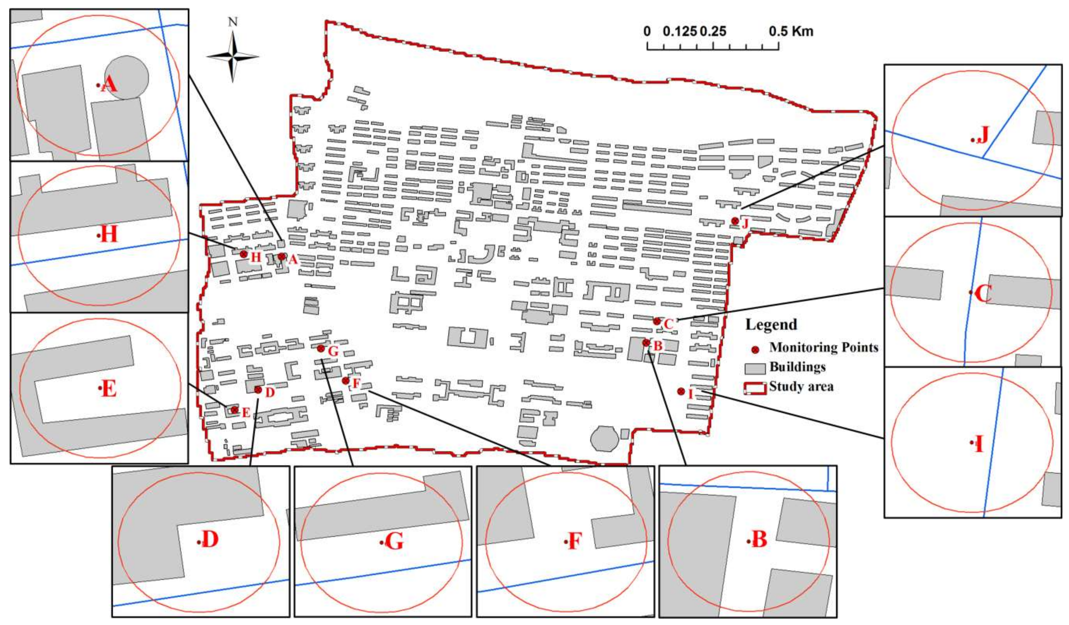
The maximum inundation depth and peak depth time were available from 10 monitoring points (points A to J) for the flood events that occurred on 1 July 2016 and 20 June 2016. The geographic information for these monitoring points is illustrated in Figure 9. The observed maximum inundation depth and peak depth time obtained from the electronic water gauge that was deployed on each monitoring point is listed in Table 1. For the flood event of 1 July 2016, it is noted that monitoring points B, C, F, and G suffered from serious inundation, with maximum water depth over 0.5 m. In particular, the inundation depth around Point B reached over 0.7 m at 9:05, which caused the severest flood inundation in study area. The flood event of 20 June 2016 also caused serious inundation at Point B, F and G, but the observed maximum inundation depths were smaller than those in flood event of 1 July 2016 on the whole. The observed data presented in Table 1 are generally consistent with the local reports regarding inundation extends and depths during each flood event. In order to describe the proximity of monitoring points to the buildings, buffer polygons were created around every monitoring point to a distance of 30 m, and the occupancy of buildings in each buffer polygon was defined as the BCR, , where and represent the building area (m2) and buffer polygon area (m2), respectively. The geospatial and geometric information of buffer polygons and the computed BCR for each monitoring point are given in Figure 9 and Table 1, respectively. The BCR of two monitoring points (points I and J) are less than 5%; these points may well be located in open areas without crowded buildings, where the building treatment method is less likely to affect the performance of the model.
2.5. Model Calibration and Validation
For inundation modeling, the study area was divided into 80 sub-catchments according to the topographic data and spatial distribution of manholes. The initial values of model parameters were evaluated based on the relationship between the empirically derived values and land-use types mentioned by the SWMM and LISFLOOD-FP user manual. Given the complexity of urban inundation modeling, the routing time step of the SWMM was set to 15 s, an adaptive time step was utilized in LISFLOOD-FP and the total simulation duration was eight hours, to include both the propagating and receding processes of the flood water. Based on the rainfall records, processed topographic data, sewer network information, and hydrological parameters within each sub-catchment, the 1D channel flows of the sewer system and the 2D floodplain flows were calculated using the dynamic wave method of SWMM and the acceleration solver of LISFLOOD-FP [43,46], respectively.
2.5.1. Calibration
The parameters of SWMM and LISFLOOD-FP were calibrated by minimizing the difference between the observed and simulated data while varying the target parameter and keeping the other constant. The objective function for calibration can be expressed as:
where RMSED (in meters) represents the root mean square error of maximum inundation depths, and describe the simulated and observed value of the maximum inundation depths, respectively, and indicates the index of the monitoring points corresponding to points A to J.
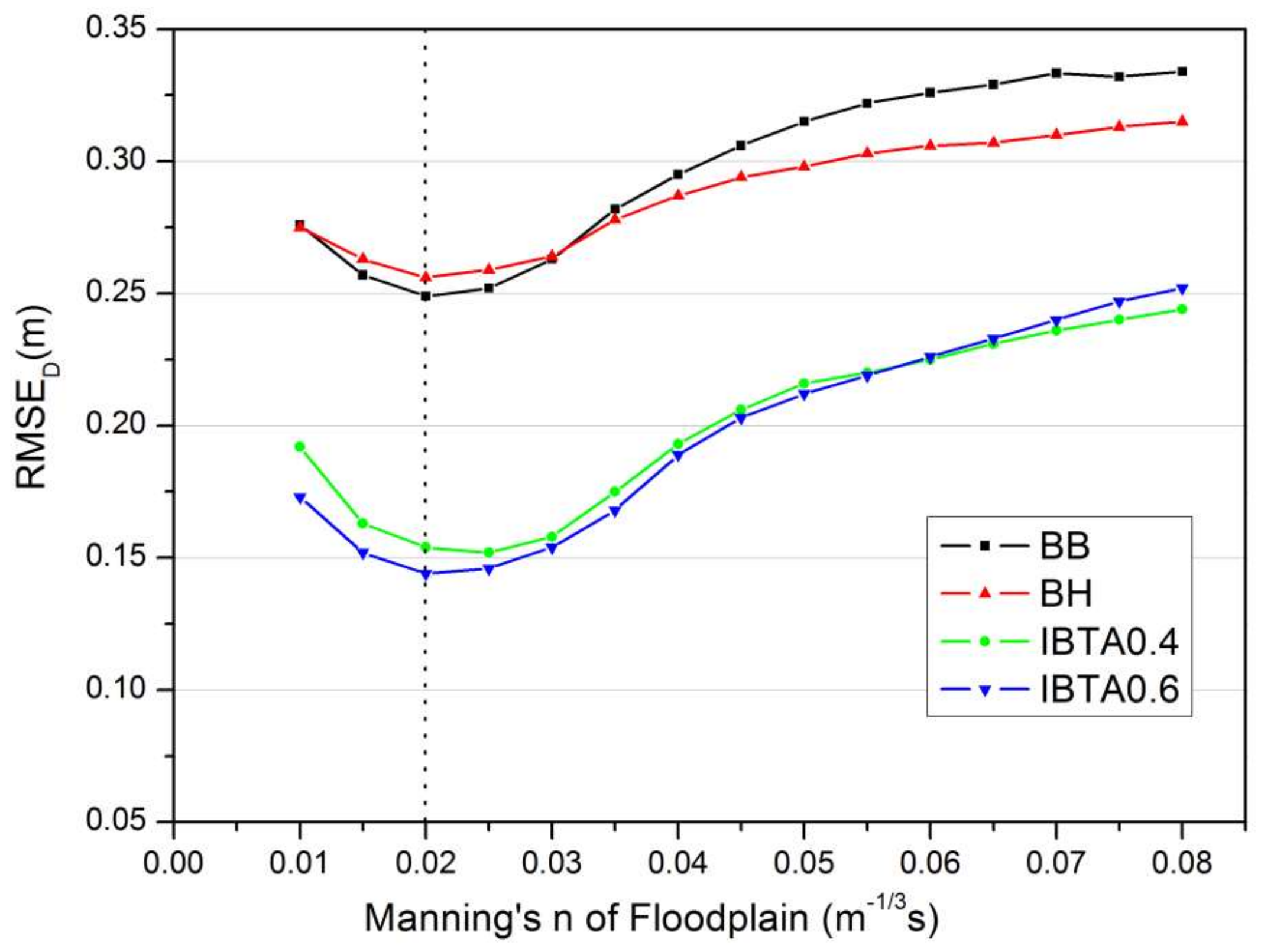
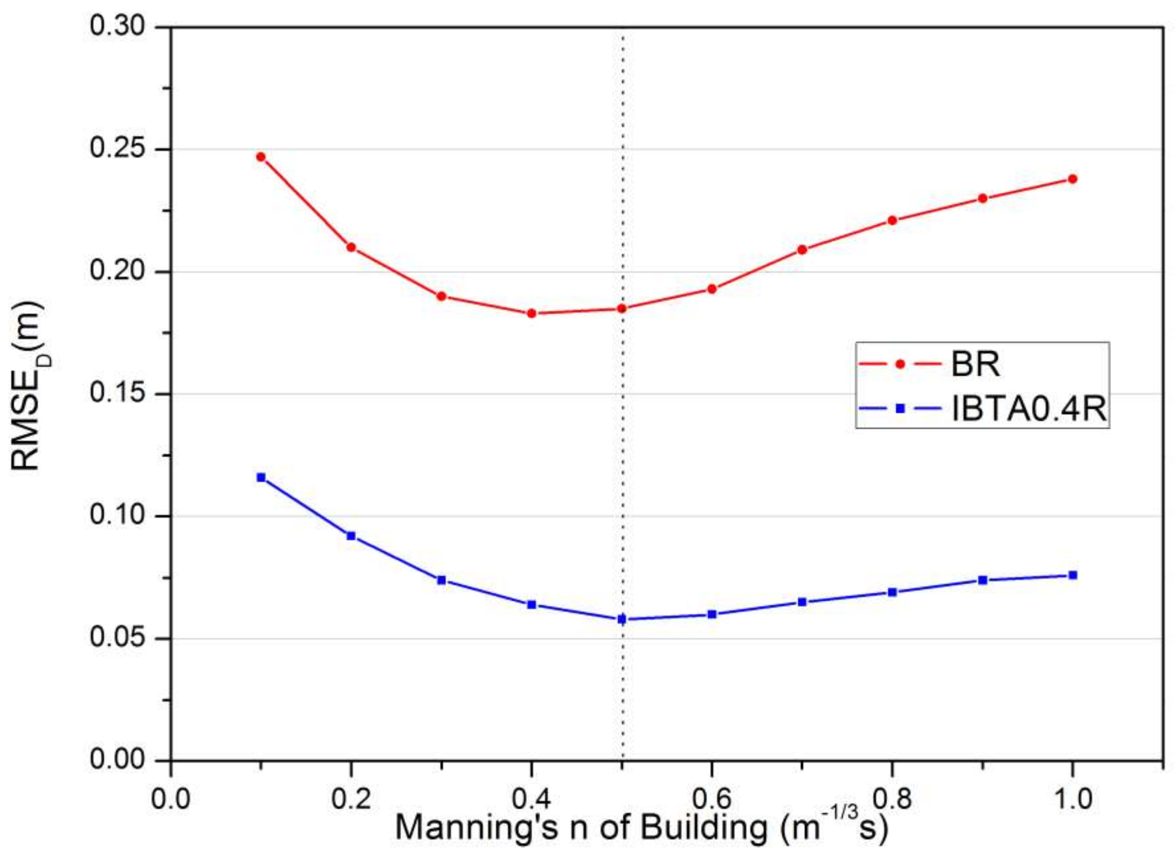
We used the flood event of 20 June 2016 to calibrate the model. Among the model parameters, the surface roughness coefficient is the most sensitive parameter relative to inundation extent and depth simulation [47]. In this study, Manning’s n for overland flow was calibrated by conducting 15 simulations for each building treatment method (except BR and IBTA0.4R) where the spatially uniform Manning’s n value varied from 0.01 to 0.08. The model response of RMSED for varying Manning’s n values of floodplain is illustrated in Figure 10. It is noted that RMSED of three methods (BB, BH and IBTA0.6) are at their minimum when n = 0.02. The sum of RMSED from all methods also reaches its minimum (0.78 m) in this case. Based on the objective function for parameter calibration, a uniform Manning’s n value of 0.02 was set as the optimal surface roughness coefficient for the entire floodplain in every building treatment method except BR and IBTA0.4R. For the BR and IBTA0.4R methods, a higher Manning’s n value of 0.5 was assigned to the areas located within the buildings, which is significantly larger than the normal value range. This value was calibrated by minimizing the sum of RMSED from BR and IBTA0.4R methods while varying the Manning’s n value of buildings from 0.1 to 1.0 and keeping the Manning’s n value of other areas at 0.02 (see Figure 11). A set of calibrated model parameters and the RMSED of each building treatment method are listed in Table 2 and Table 3, respectively. It is noted that the traditional methods (BB, BH and BR) produced relatively poor performance in term of maximum inundation depth, with RMSED all greater than 0.18 m. This might be because these methods were limited in correctly describing the influence of buildings on surface flows. To investigate this, the RMSED of each building treatment method were calculated again based on the simulated and observed data from two monitoring points (points I and J) that are located in open areas without crowded buildings, and the results can be found in Table 3. Note that a high level of agreement between simulated and observed inundation depth was achieved by every method at points I and J, with RMSED smaller than 0.06 m. In view of this, the calibrated parameters were considered suitable for inundation modeling.
2.5.2. Validation
The 1 July 2016 flood event was used as the case event to validate the models using different building treatment methods. Same objective function as the calibration was applied to the validation process. RMSED was chosen as the indicator to assess the performance of proposed IBTA and traditional methods. The validation results of each building treatment method are given in Table 3. The IBTA0.4R method was tested to produce a preferable simulation of maximum inundation depth than the other methods. Similar to the calibration process, high RMSED can be found in the validation results produced by the traditional methods. However, we also found that the simulated maximum inundation depth at points I and J matched well with the observed data in every method, with RMSED smaller than 0.07 m. These results imply that poor performance of the traditional method was more likely to be due to the limited representation of building effects than to the unsuitable model parameters. Therefore, the model parameters were deemed applicative in the study area. In addition, detailed information for the validation results and performance of each building treatment method will be presented and discussed in Section 3.2.
3. Results and Discussions
3.1. Model Sensitivity to Building Treatment Method
We used the 1 July 2016 flood event to investigate the model sensitivity to building treatment method. Figure 12 illustrates the simulation results of the 1D channel flows of the sewer system produced by SWMM in the flood event of 1 July 2016. The surcharged flow appears in 83 manholes, which constitute the flooding sources of the surface inundation.
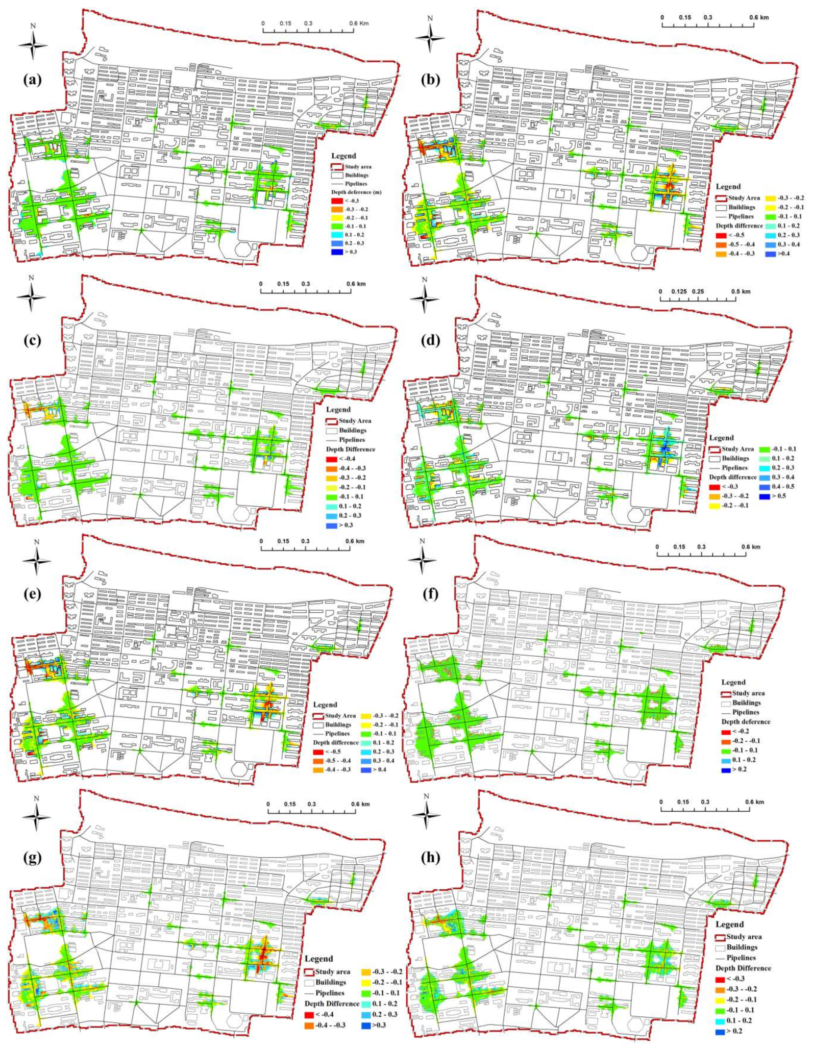
A summary of the maximum flood area and the inundation depth simulated by the models using different building treatment methods are presented in Figure 13. DEM cells that were simulated to be wet are rendered by different blue colors according to the maximum inundation depths, while cells with no color are dry. Overall, the size and shape of the inundation area resulting from each modeling scenario are similar. The wet cells mainly propagate along roads and accumulate in the southwestern and southeastern districts of the study area, which have low-lying topographies, and are generally consistent with the observed inundation zone accounts collected from eyewitnesses and historical photography within regions A to D in the flood event of 1 July 2016, as shown in Figure 13a. It appears that the simulated inundation area is characterized by an acceptable degree of consistency among all the modeling scenarios. As mentioned before, the simulated flood area is difficult to validate due to a lack of suitable observation data for the flood event, so the overall flood area and inundation depth differences between the modeling scenarios provided by each building treatment method were computed to reveal the model sensitivity to the building treatment method. A subset of results is given in Figure 14 and is described as follows.
- BB-BH methods: No remarkable difference in maximum inundation extent could be found between the BH and BB methods. Both methods present extensive and torrential inundation within regions A to D (see Figure 13a,b). Nevertheless, the BH method produces a slightly smaller inundation zone compared to the BB method along the western and southern edge of region C (Figure 14a). Moreover, the BH method produces a slightly larger maximum inundation depth compared to the BB method along the building footprints and gaps, especially in regions A and D with dense building coverage. Considering the small distinction between the BH and BB simulations, the BB method serves as the benchmark of these two methods when compared to other methods.
- IBTA0.4-BB methods: There are significant differences in the simulated maximum inundation area and depth between the IBTA0.4 and BB methods (see Figure 13a,c and Figure 14b). The BB method generally produces higher inundation depths than IBTA0.4, particularly for the area between the crowded buildings alongside the road. Specifically, the BB method demonstrates a torrential inundation at Nanyi Road (region A), which is surround by cafeterias and apartment buildings, and the highest inundation depth reaches over 0.8 m (Figure 13a). On the other hand, Nanyi Road is flooded by water with a maximum inundation depth below 0.6 m in the modeling scenario simulated by IBTA0.4. Similar differences can be found around the Coal Combustion Laboratory in the southwest corner of region C. The BB method simulated much higher inundation depths in the recess of the laboratory building than IBTA0.4. Furthermore, in the IBTA0.4 simulation, we note that fair amounts of the area within the buildings are simulated to be wet, which is not the case in BB simulations. The discrepancies in simulations of localized inundation area and depth are attributed to the different values of building elevation used in these two methods. For IBTA0.4, the inner areas of the buildings are available for storage when the inundation depth rises to 0.4 m, while the flow water is still confined between the outer walls of buildings in the BB method, leading to the increase in water depths. Additionally, we note that IBTA0.4 also simulates smaller maximum inundation area and depths at Xiwu Road, which is located at the western edge of region A and intersects with Nanyi Road at its western endpoint. This is primarily because the buildings alongside Nanyi Road act to redirect the southward- and northward-moving surface flow to the west in the BB method; therefore, more water reaches Xiwu Road in this case. These results indicate that the localized simulated inundation areas and depths are sensitive to the building treatment method.
- IBTA0.6-BB methods: As shown in Figure 13a,d and Figure 14c, the IBTA0.6 and BB methods also produce varying simulated maximum inundation areas and depths. The greatest differences between the two methods also occurred mainly at locations near dense buildings in regions A and D, yet to a smaller degree than that in Figure 14b. Moreover, the simulated maximum inundation area and depths of IBTA0.6 agree well with those of the BB method in most of regions B and C, which is markedly different from the results shown in Figure 14b. This is because, for the IBTA0.6 method, the simulated maximum inundation depth in most parts of regions B and C is below 0.6 m, in which case the buildings are still treated as a solid block, and results in similar inundation depths to the BB method. Nevertheless, as shown by the discrepancies in the simulation results illustrated in Figure 14c, the model sensitivity to the building treatment method becomes more pronounced.
- IBTA0.6-IBTA0.4 methods: There are considerable differences in both maximum inundation area and depth between the IBTA0.6 and IBTA0.4 simulations, and especially in the local areas around the building features (Figure 13c,d and Figure 14d). Overall, IBTA0.6 produces deeper flood water along the road, but shallower or no inundation inside buildings, compared to the IBTA0.4 method. This is attributed to the increase in threshold of building entrance height (from 0.4 m to 0.6 m) when the IBTA0.6 method is used. With the increase of building elevation, less flux enters the buildings, and the overlooked building storage volume leads to increased pooling along the road and in other lowlands outside of building, thus resulting in more severe inundation. Therefore, it can be inferred that the storage and blockage effects of buildings are affected by the changes in threshold used for terrain preprocessing.
- IBTA0.4R-IBTA0.4 methods: The simulated maximum inundation areas and depths differ very little between the IBTA0.4R and IBTA0.4 methods, except in some areas within and along the building footprints where patches of red and blue colors appear in Figure 14f. IBTA0.4R always produces greater inundation depths but smaller flooding extent inside buildings than the IBTA0.4 method. This is ascribed to the building resistance effect represented in the IBTA0.4R method by changing the Manning’s n value at building’s position, in which case water flow into buildings is inhibited by the presence of inner walls, furniture and closed doors. It can be inferred that beyond the storage and blockage effect, the inner resistance effect of the buildings should also not be ignored in urban inundation modeling.
- BR-IBTA0.6 methods: Remarkable differences in the simulated maximum inundation area and depth can be found between the modeling scenarios of BR and IBTA0.6, particularly in the dense building areas of regions A and D (see Figure 14g). The BR method generally produces smaller maximum inundation depths than IBTA0.6 along the roads and alleyways between densely-spaced buildings, but higher inundation depths inside buildings. This is a result of the absence of building blockage effect in the BR method. In IBTA0.6, DEM cells fall within building features and can obstruct flow and block flood flows from reaching the interior spaces of the buildings when the water level is below 0.6 m, in contrast to the BR method which can only resist flow. In the BR method, significant volumes of water enter and move through the buildings without any solid obstruction. Therefore, less water accumulates and flows along the roads and alleyways between buildings, leading to lower inundation depths.
- BR-IBTA0.4R methods: As shown in Figure 14h, the differences in the simulated maximum inundation area and depth between BR and IBTA0.4R methods are smaller than those in Figure 14g, especially in region D with dense building coverage. This is mainly because the building blockage effect is decreased in IBTA0.4R by using a lower threshold of building entrance height. It can be seen from Figure 13 and Figure 14 that as the full grid area remains available for water storage, the BR method generally simulates lower inundation depth and greater lateral spreading than the other methods. These results are similar to those of Schubert and Sanders [36], suggesting the significant role played by solid obstruction in the flood wave propagation and the importance of an accurate representation of building blockage effect in urban inundation modeling.
3.2. Performance of Building Treatment Methods
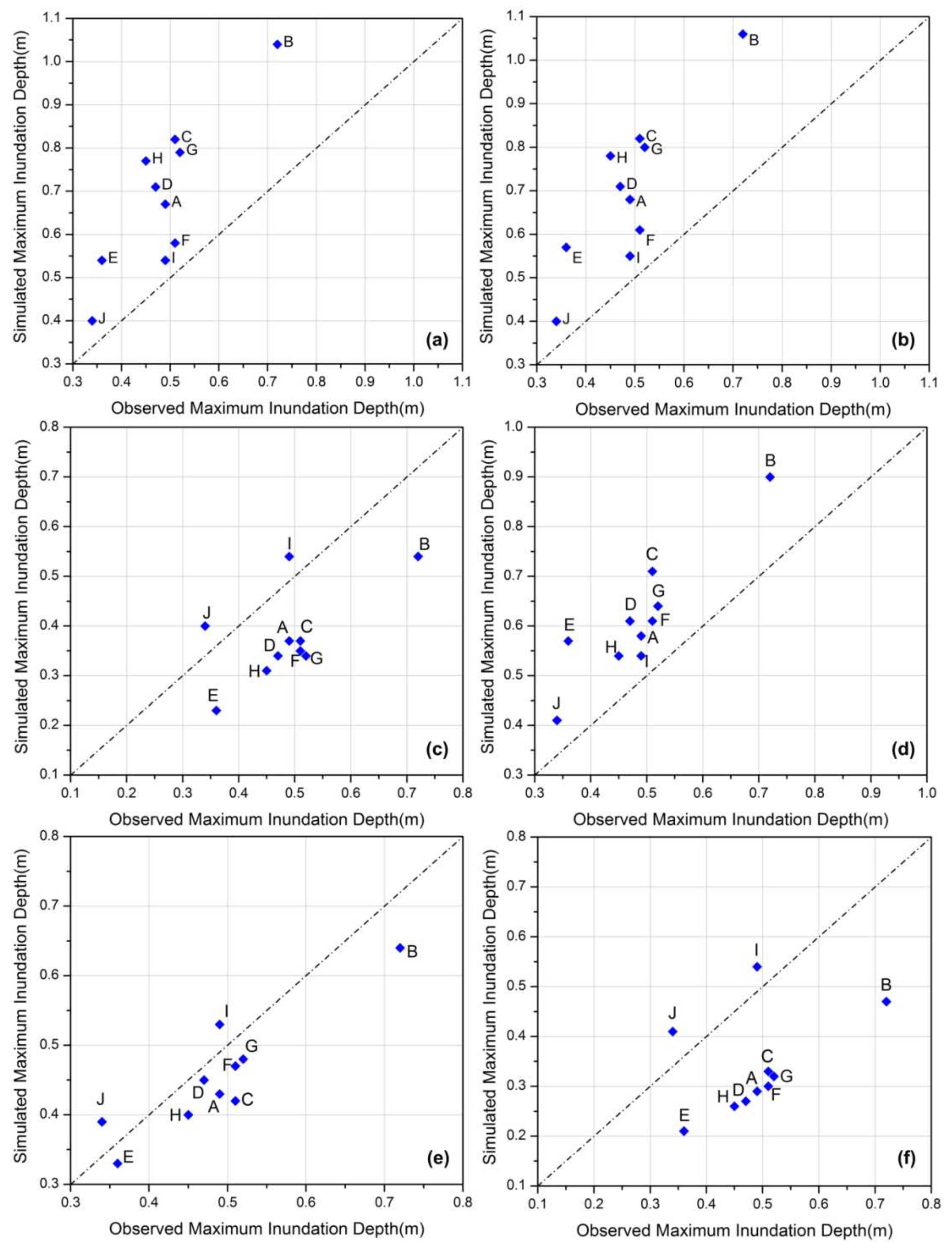
Figure 15 shows the model performance of each building treatment method in term of maximum inundation depth at each monitoring point (from points A to J) when compared to the observed data from the flood event of 1 July 2016.
Figure 15a,b reveal an overall overestimation of maximum inundation depth in both the BB and BH methods, with RMSED values of 0.23 m and 0.24 m, respectively. This may be attributed to the absence of the building storage effect in the BH and BB methods, particularly for the monitoring points falling within the dense building area (from points A to H). For instance, for monitoring Point H, which is located in the mid-western part of Region A, the maximum inundation depth produced by the BB method (0.77 m) and obtained from the observations (0.45 m) differ by up to 71%. This suggests that in the BB method, as the building elevations are much higher than the nearby ground elevations, more water accumulates along the roads and other lowlands due to the existence of dense buildings, which, in turn, leads to unrealistically high inundation depths. Similar to the BH and BB methods, overestimation of the maximum inundation depth occurs in the IBTA0.6 method (Figure 15d), however to a lower degree, with a RMSED of 0.14 m. As mentioned before, this is probably because the storage effect of buildings is reduced by higher building elevation, and in most cases the buildings still act as obstructions to the surface flow. On the other hand, as demonstrated in Figure 15c, there is an overall underestimation of maximum inundation depth in the IBTA0.4 method, with a RMSED of 0.14 m. This is ascribed to the limited representation of the water resistance effect inside buildings when the IBTA0.4 method is used. Once floodwater enters the buildings, it can rapidly flow through the rooms toward garden spaces behind buildings without any obstacles, which results in a larger inundation area and lower flood depth. Two outliers are noted, including the simulations at points I and J, which calls for deeper inundations than the observations that are similar to BH, BB, and IBTA0.6. Similar underestimation of maximum inundation depth can be found to an even higher degree in the BR method (see Figure 15f), with a RMSED of 0.18 m. This may be a result of the loss of building blockage effect in the BR method, in which case the building feature can no longer obstruct but only resist the surface flow. The underestimations in the IBTA0.4 and BR methods are improved by applying higher Manning’s n values and elevations to the areas covered by buildings in IBTA0.4R, as shown in Figure 15e. Compared to other methods, simulated inundation depth resulting from the IBTA0.4R method is characterized by a high degree of consistency with the observation and the smallest magnitude of RMSED (0.06 m). This result confirms that the potential storage capacity and drag resistance inside buildings are not negligible in urban inundation modeling, and the model performance of inundation depth can be improved by better representing both blockage, storage, and resistance effects of buildings.
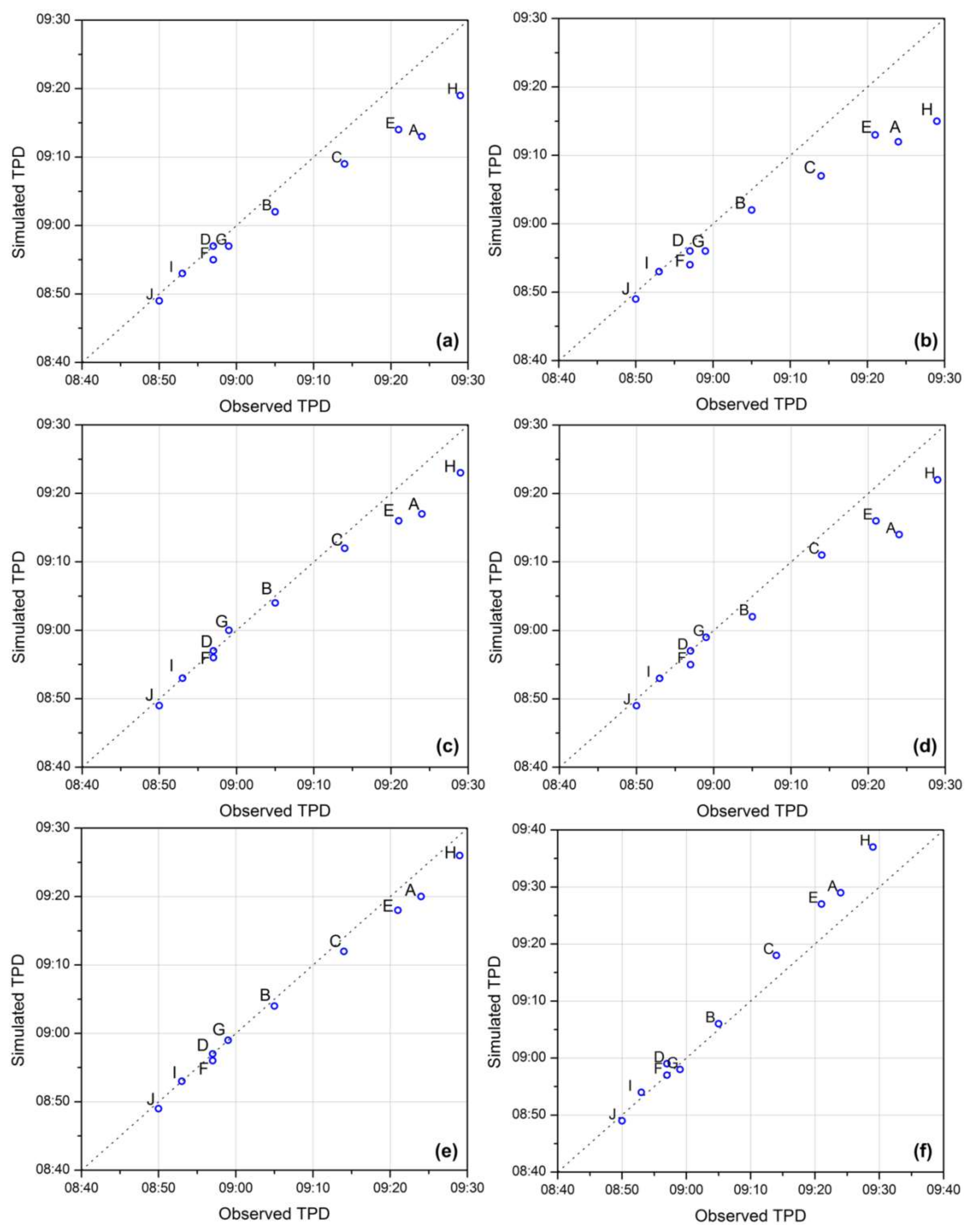
Figure 16 gives a comparison of the observations and the simulated timing of peak depth (TPD) at each monitoring point (from points A to J) resulted from varying building treatment methods. RMSET was chosen as the indicator to assess the performance of TPD for each modeling scenario. RMSET (in meters) is the root mean square error of TPD and can be calculated as follows:
where and represent the simulated and observed peak depth time, respectively, and indicates the index of the monitoring points corresponding to points A to J.
As shown in Figure 16a,b, the BH and BB methods tend to produce peak depths that occur earlier than the observations with RMSET of approximately six and seven minutes, respectively. The differences are larger at points A, E, and H, which are located within dense building areas. This is because the flood water is confined between crowded buildings alongside the road in the BH and BB methods, thus leading to high velocity flows along the roadways and earlier occurrences of maximum inundation depth. Improved results can be found in the simulations produced by IBTA0.4 and IBTA0.6 (Figure 16c,d), with RMSET values of approximately 3 min and 4 min, respectively. However, the peak inundation depths still occur in advance at the monitoring points located in dense building areas. As shown in Figure 16e, the peak depth time produced by IBTA0.4R match well with the observations with no significant outliers, and the RMSET of IBTA0.4R is less than 2 min. This may be attributed to the building resistance effect represented by the IBTA0.4R method, which can reduce the propagation velocity of the flood wave around buildings and delay the occurrences of maximum inundation depth at points A, E, and H. In contract to all other methods, the BR method generally produces peak depths that occur later than the observations with RMSET of approximately 4 min. This is possibly due to the absence of solid obstruction and higher friction parameters used for the building areas in the BR method, which reduce the flow rate into and out of buildings and delay the appearances of peak inundation depth. Moreover, the timings of peak inundation depths at points J, I and D are simulated well in every modeling scenario. This is probably because of the short distances between these monitoring points and the flooding sources. Based on the results that are shown in Figure 15 and Figure 16, we can conclude that improved performance in terms of maximum inundation depths and peak depth time can be obtained when using the IBTA0.4R method, in which the blockage, storage and resistance effects caused by dense buildings are adequately represented.
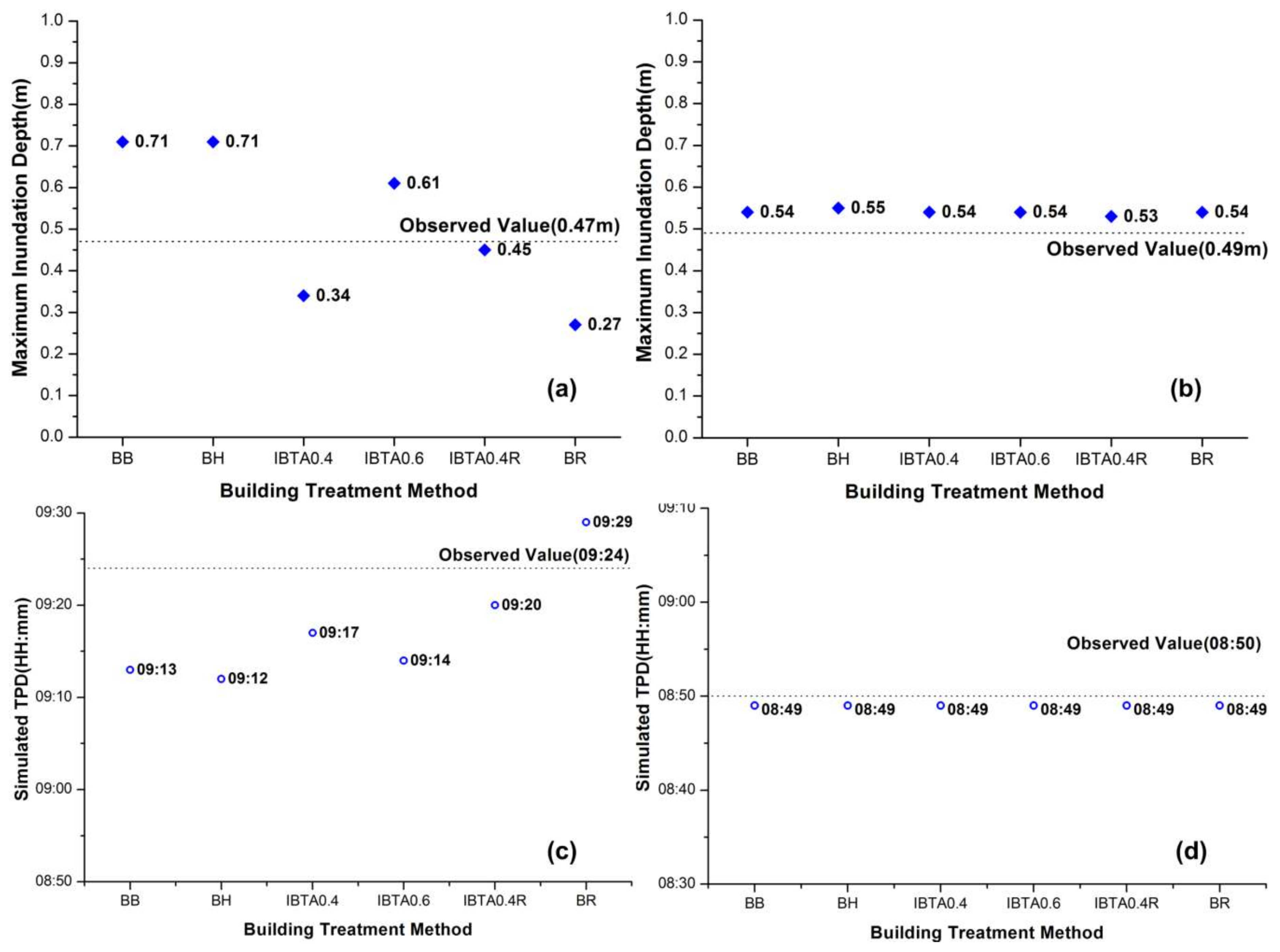
To explore the spatiotemporal inhomogeneity of model sensitivity to building treatment methods, comparisons of the simulations produced by the different modeling scenarios and the observed values at four single monitoring points are plotted in Figure 17. According to the computed BCR for each monitoring point listed in Table 1, it is noted that two of these points (points A and D) are located in dense building areas, and two others (points I and J) are located in open areas without crowded buildings. The results illustrated in Figure 17 suggest that the simulated maximum inundation depths and their timing generally vary with the building treatment methods at points A and D, whereas these simulation results are mostly unchanged at points I and J when different methods are applied. Based on the results demonstrated in Figure 15, Figure 16 and Figure 17, we found that the simulated maximum inundation depth and peak depth time at points I and J match well with the observations in all modeling scenarios. A high level of agreement (RMSED < 0.07 m and RMSET < 1 min) is achieved by every building treatment method at these two points. Therefore, it can be inferred that simulated maximum inundation depth and timing are sensitive to the building treatment method used in dense building regions, but seemingly insensitive in open areas away from buildings.
4. Conclusions
In this study, we considered both the blockage effect and storage capacity of buildings and described an improved building treatment approach (IBTA) for representing urban structures. In this approach, we applied smaller building elevations (0.4 m and 0.6 m above the local ground level elevation) than in the BB method, which can prevent water from flowing into the buildings until the water depth is sufficient to exceed the threshold of building entrance height. Moreover, the inner resistance effect of buildings was also represented in IBTA0.4R by applying a higher Manning’s n value to the areas covered by buildings.
To test the model’s ability to represent buildings, comparison analyses were carried out based on the inundation simulations provided by the proposed IBTA (IBTA0.4, IBTA0.6, and IBTA0.4R) and traditional (BB, BH, and BR) methods for the flood events that occurred in the study area. The results can be concluded as follows:
- The model results of the maximum inundation depth, extent and timing of the peak depth all exhibited sensitivity to the building treatment method in dense building regions of the study area. However, this sensitivity is reduced in open areas without dense building surroundings (points I and J).
- As the blockage, storage and resistance effects of buildings were both adequately represented, IBTA0.4R produced the best performance across all building treatment methods considered in this study when assessed against the measurement values of the flood event.
The lack of detailed observed data, especially the inundation area and surface flow data, will undoubtedly challenge the calibration and validation of the IBTA. However, improved representation of flood dynamics around dense buildings in IBTA0.4R can still be verified based on the observed maximum inundation depth and peak depth time obtained from 10 monitoring points in the study area. Therefore, this study provides a new approach to simulate the flood wave propagation and the inundation for densely built urban areas. To determine accepted guidelines for building treatments in flood inundation modeling, future works should concentrate on further verifying the performance of the IBTA in other urban environments where precise measurements of surface flow are available for model calibration and validation. The proposed IBTA should be applied cautiously in other urban settings for now.
Author Contributions
J.S. conceived and designed the improved building treatment approach. Y.Z. performed the rainfall-runoff model and evaluated the flood volumes. F.T. designed and performed the comparison experiments. All authors discussed the results and wrote the manuscript.
Funding
This research was funded by National Natural Science Foundation of China, grant number 61602518.
Acknowledgments
The authors would like to appreciate the supports for this study from the National Natural Science Foundation of China (no. 41101258 and 61602518) and the National Key Technology R and D Program of China (no. 2008BAC36B01). The authors also greatly appreciate the anonymous reviewers and academic editor for their careful comments and valuable suggestions to improve the manuscript.
Conflicts of Interest
The authors declare no conflict of interest.
References
- Hsu, M.H.; Chen, S.H.; Chang, T.J. Inundation simulation for urban drainage basin with storm sewer system. J. Hydrol. 2000, 234, 21–37. [Google Scholar] [CrossRef] [Green Version]
- Wu, X.; Yu, D.; Wilby, R.L. An evaluation of the impacts of land surface modification, storm sewer development, and rainfall variation on waterlogging risk in Shanghai. Nat. Hazards 2012, 63, 305–323. [Google Scholar] [CrossRef]
- Yin, J.; Yu, D.; Yin, Z.; Wang, J.; Xu, S. Modelling the anthropogenic impacts on fluvial flood risks in a coastal mega-city: A scenario-based case study in Shanghai, China. Landsc. Urban Plan. 2015, 136, 144–155. [Google Scholar] [CrossRef]
- Gallegos, H.A.; Schubert, J.E.; Sanders, B.F. Two-dimensional, high-resolution modeling of urban dam-break flooding: A case study of Baldwin Hills, California. Adv. Water Resour. 2009, 32, 1323–1335. [Google Scholar] [CrossRef]
- Tsubaki, R.; Fujita, I. Unstructured grid generation using LiDAR data for urban flood inundation modelling. Hydrol. Process. 2010, 24, 1404–1420. [Google Scholar] [CrossRef]
- Du, J.; Qian, L.; Rui, H.; Zuo, T.; Zheng, D.; Xu, Y.; Xu, C. Assessing the effects of urbanization on annual runoff and flood events using an integrated hydrological modeling system for Qinhuai River basin, China. J. Hydrol. 2012, 464, 127–139. [Google Scholar] [CrossRef]
- Alfieri, L.; Feyen, L.; Baldassarre, G.D. Increasing flood risk under climate change: A pan-European assessment of the benefits of four adaptation strategies. Clim. Chang. 2016, 136, 507–521. [Google Scholar] [CrossRef] [Green Version]
- Kelman, I.; Spence, R. An overview of flood actions on buildings. Eng. Geol. 2004, 73, 297–309. [Google Scholar] [CrossRef]
- Middelmann-Fernandes, M.H. Flood damage estimation beyond stage–damage functions: An Australian example. J. Flood Risk Manag. 2010, 3, 88–96. [Google Scholar] [CrossRef]
- Fewtrell, T.J.; Bates, P.D.; Horritt, M.; Hunter, N.M. Evaluating the effect of scale in flood inundation modelling in urban environments. Hydrol. Process. 2010, 22, 5107–5118. [Google Scholar] [CrossRef]
- Biancamaria, S.; Bates, P.D.; Boone, A.; Mognard, N.M. Large-scale coupled hydrologic and hydraulic modelling of the Ob river in Siberia. J. Hydrol. 2009, 379, 136–150. [Google Scholar] [CrossRef] [Green Version]
- Yu, D.; Lane, S.N. Interactions between subgrid-scale resolution, feature representation and grid-scale resolution in flood inundation modelling. Hydrol. Process. 2011, 25, 36–53. [Google Scholar] [CrossRef] [Green Version]
- Mignot, E.; Paquier, A.; Haider, S. Modeling floods in a dense urban area using 2D shallow water equations. J. Hydrol. 2006, 327, 186–199. [Google Scholar] [CrossRef] [Green Version]
- Hine, D.; Hall, J.W. Information gap analysis of flood model uncertainties and regional frequency analysis. Water Resour. Res. 2010, 46, W01514. [Google Scholar] [CrossRef]
- Phillips, B.C.; Yu, S.; Thompson, G.R.; De Silva, N. 1D and 2D Modelling of Urban Drainage Systems using XP-SWMM and TUFLOW. In Proceedings of the 10th International Conference on Urban Drainage, Copenhagen, Denmark, 21–26 August 2005; pp. 21–26. [Google Scholar]
- Mciwem, K.B. JFLOW: A multiscale two-dimensional dynamic flood model. Water Environ. J. 2010, 20, 79–86. [Google Scholar]
- Bates, P.D.; De Roo, A.P.J. A simple raster-based model for flood inundation simulation. J. Hydrol. 2000, 236, 54–77. [Google Scholar] [CrossRef]
- Lamb, R.; Crossley, A.; Waller, S. A fast 2D floodplain inundation model. Water Manag. 2009, 162, 363–370. [Google Scholar]
- Neal, J.; Schumann, G.; Bates, P.D. A subgrid channel model for simulating river hydraulics and floodplain inundation over large and data sparse areas. Water Resour. Res. 2012, 48, W11506. [Google Scholar] [CrossRef]
- Schumann, J.P.; Neal, J.C.; Voisin, N.; Andreadis, K.M.; Pappenberger, F.; Phanthuwongpakdee, N.; Hall, A.C.; Bates, P.D. A first large-scale flood inundation forecasting model. Water Resour. Res. 2013, 49, 6248–6257. [Google Scholar] [CrossRef] [Green Version]
- Neal, J.; Schumann, G.; Fewtrell, T.; Budimir, M.; Bates, P.D.; Mason, D. Evaluating a new LISFLOOD-FP formulation with data from the summer 2007 floods in Tewkesbury, UK. J. Flood Risk Manag. 2011, 4, 88–95. [Google Scholar] [CrossRef]
- Mason, D.C.; Cobby, D.M.; Horritt, M.S.; Bates, P.D. Floodplain friction parameterization in two-dimensional river flood models using vegetation heights derived from airborne scanning laser altimetry. Hydrol. Process. 2003, 17, 1711–1732. [Google Scholar] [CrossRef]
- Fewtrell, T.J.; Duncan, A.; Sampson, C.C.; Neal, J.C.; Bates, P.D. Benchmarking urban flood models of varying complexity and scale using high resolution terrestrial LiDAR data. Phys. Chem. Earth 2011, 36, 281–291. [Google Scholar] [CrossRef]
- Sampson, C.C.; Fewtrell, T.J.; Duncan, A.; Shaad, K.; Horritt, M.S.; Bates, P.D. Use of terrestrial laser scanning data to drive decimetric resolution urban inundation models. Adv. Water Resour. 2012, 41, 1–17. [Google Scholar] [CrossRef]
- Ozdemir, H.; Sampson, C.C.; De Almeida, G.A.M.; Bates, P.D. Evaluating scale and roughness effects in urban flood modelling using terrestrial LIDAR data. Hydrol. Earth Syst. Sci. 2013, 17, 4015–4030. [Google Scholar] [CrossRef] [Green Version]
- Neal, J.; Villanueva, I.; Wright, N.; Willis, T.; Fewtrell, T.; Bates, P.D. How much physical complexity is needed to model flood inundation? Hydrol. Process. 2012, 26, 2264–2282. [Google Scholar] [CrossRef]
- Yin, J.; Lin, N.; Yu, D. Coupled modeling of storm surge and coastal inundation: A case study in New York City during Hurricane Sandy. Water Resour. Res. 2016, 52, 8685–8699. [Google Scholar] [CrossRef] [Green Version]
- Gallien, T.W.; Schubert, J.E.; Sanders, B.F. Predicting tidal flooding of urbanized embayments: A modeling framework and data requirements. Coast. Eng. 2011, 58, 567–577. [Google Scholar] [CrossRef]
- Brown, J.D.; Spencer, T.; Moeller, I. Modeling storm surge flooding of an urban area with particular reference to modeling uncertainties: A case study of Canvey Island, United Kingdom. Water Resour. Res. 2007, 43, 93–104. [Google Scholar] [CrossRef]
- Schubert, J.E.; Sanders, B.F.; Smith, M.J.; Wright, N.G. Unstructured mesh generation and landcover-based resistance for hydrodynamic modeling of urban flooding. Adv. Water Resour. 2008, 31, 1603–1621. [Google Scholar] [CrossRef]
- Hunter, N.M.; Bates, P.D.; Neelz, S.; Pender, G.; Villanueva, I.; Wright, N.G.; Liang, D.; Falconer, R.A.; Lin, B.; Waller, S.; et al. Benchmarking 2D Hydraulic Models for Urban Flood Simulations. Water Manag. 2008, 161, 13–30. [Google Scholar]
- Aronica, G.T.; Lanza, L.G. Drainage efficiency in urban areas: A case study. Hydrol. Process. 2010, 19, 1105–1119. [Google Scholar] [CrossRef]
- Aronica, G.T.; Tucciarelli, T.; Nasello, C. 2D Multilevel Model for Flood Wave Propagation in Flood-Affected Areas. J. Water Resour. Plan. Manag. 1998, 124, 210–217. [Google Scholar] [CrossRef]
- Chen, A.S.; Evans, B.; Djordjević, S.; Savic, D.A. A coarse-grid approach to representing building blockage effects in 2D urban flood modelling. J. Hydrol. 2012, 426, 1–16. [Google Scholar] [CrossRef] [Green Version]
- Chen, A.S.; Evans, B.; Djordjević, S.; Savic, D.A. Multi-layered coarse grid modelling in 2D urban flood simulations. J. Hydrol. 2012, 470, 1–11. [Google Scholar] [CrossRef] [Green Version]
- Schubert, J.E.; Sanders, B.F. Building treatments for urban flood inundation models and implications for predictive skill and modeling efficiency. Adv. Water Resour. 2012, 41, 49–64. [Google Scholar] [CrossRef]
- Wu, X.; Wang, Z.; Guo, S.; Liao, W.; Zeng, Z.; Chen, X. Scenario-based projections of future urban inundation within a coupled hydrodynamic model framework: A case study in Dongguan City, China. J. Hydrol. 2017, 547, 428–442. [Google Scholar] [CrossRef]
- Schmitt, T.G.; Thomas, M.; Ettrich, N. Analysis and modeling of flooding in urban drainage systems. J. Hydrol. 2004, 299, 300–311. [Google Scholar] [CrossRef]
- Leandro, J.; Chen, A.S.; Djordjevic, S.; Savic, D.A. Comparison of 1D/1D and 1D/2D coupled (sewer/surface) hydraulic models for urban flood simulation. J. Hydraul. Eng. 2009, 135, 495–504. [Google Scholar] [CrossRef]
- Peterson, E.W.; Wicks, C.M. Assessing the importance of conduit geometry and physical parameters in karst systems using the storm water management model (SWMM). J. Hydrol. 2006, 329, 294–305. [Google Scholar] [CrossRef]
- Gironás, J.; Roesner, L.A.; Rossman, L.A.; Davis, J. A new applications manual for the Storm Water Management Model (SWMM). Environ. Model. Softw. 2010, 25, 813–814. [Google Scholar] [CrossRef]
- Hunter, N.M.; Horritt, M.S.; Bates, P.D.; Wilson, M.D.; Werner, M.G.F. An adaptive time step solution for raster-based storage cell modelling of floodplain inundation. Adv. Water Resour. 2005, 28, 975–991. [Google Scholar] [CrossRef]
- Bates, P.D.; Horritt, M.S.; Fewtrell, T.J. A simple inertial formulation of the shallow water equations for efficient two-dimensional flood inundation modelling. J. Hydrol. 2010, 387, 33–45. [Google Scholar] [CrossRef]
- Dottori, F.; Todini, E. Developments of a flood inundation model based on the cellular automata approach: Testing different methods to improve model performance. Phys. Chem. Earth 2011, 36, 266–280. [Google Scholar] [CrossRef]
- Sampson, C.C.; Bates, P.D.; Neal, J.C.; Horritt, M.S. An automated routing methodology to enable direct rainfall in high resolution shallow water models. Hydrol. Process. 2013, 27, 467–476. [Google Scholar] [CrossRef]
- De Almeida, G.A.M.; Bates, P.D. Applicability of the local inertial approximation of the shallow water equations to flood modeling. Water Resour. Res. 2013, 49, 4833–4844. [Google Scholar] [CrossRef] [Green Version]
- Yu, D.; Coulthard, T.J. Evaluating the importance of catchment hydrological parameters for urban surface water flood modelling using a simple hydro-inundation model. J. Hydrol. 2015, 524, 385–400. [Google Scholar] [CrossRef] [Green Version]
Figure 1.
Terrain preprocessing method used in IBTA.

Figure 2.
Study area: The main campus of Huazhong University of Science and Technology (HUST) in Wuhan City, China. The four regions that were reported to be most at risk from surface water flooding were: A—Nanyi Road; B—Zisong Road; C—Laboratory of Coal Combustion; and D—Doctor Apartment.
Figure 2.
Study area: The main campus of Huazhong University of Science and Technology (HUST) in Wuhan City, China. The four regions that were reported to be most at risk from surface water flooding were: A—Nanyi Road; B—Zisong Road; C—Laboratory of Coal Combustion; and D—Doctor Apartment.

Figure 3.
The coupled urban flood inundation simulation model used in this study.

Figure 4.
Rainfall records of the flood events that occurred on 20 June 2016 (a) and 1 July 2016 (b) at Wuhan City.
Figure 4.
Rainfall records of the flood events that occurred on 20 June 2016 (a) and 1 July 2016 (b) at Wuhan City.

Figure 5.
The bare-earth DEM of the study area (a), and the topographic processing results for each building treatment method: (b) the BB method; (c) the BH method; (d) the IBTA0.4 method; and (e) the IBTA0.6 method.
Figure 5.
The bare-earth DEM of the study area (a), and the topographic processing results for each building treatment method: (b) the BB method; (c) the BH method; (d) the IBTA0.4 method; and (e) the IBTA0.6 method.

Figure 6.
The geometry of buildings in the study area.

Figure 7.
Histogram of building parameters in the study area: (a) building sizes and gaps; and (b) building entrance heights.
Figure 7.
Histogram of building parameters in the study area: (a) building sizes and gaps; and (b) building entrance heights.

Figure 8.
Geospatial and geometric information of the storm sewer system in the study area.

Figure 9.
Geographic information of monitoring points in study area.

Figure 10.
Model response of RMSED for varying Manning’s n value of floodplain. The dotted line represents the optimal Manning’s n value of floodplain used in this study.
Figure 10.
Model response of RMSED for varying Manning’s n value of floodplain. The dotted line represents the optimal Manning’s n value of floodplain used in this study.

Figure 11.
Model response of RMSED for varying Manning’s n value of buildings. The dotted line represents the optimal Manning’s n value of buildings used in the BR and IBTA0.4R methods.
Figure 11.
Model response of RMSED for varying Manning’s n value of buildings. The dotted line represents the optimal Manning’s n value of buildings used in the BR and IBTA0.4R methods.

Figure 12.
Simulation results of the 1D channel flows of the sewer system.

Figure 13.
Maximum flood area and inundation depth simulated by the models using different building treatments: (a) BB Method; (b) BH method; (c) IBTA0.4 method; (d) IBTA0.6 method; (e) IBTA0.4R method; and (f) BR method.
Figure 13.
Maximum flood area and inundation depth simulated by the models using different building treatments: (a) BB Method; (b) BH method; (c) IBTA0.4 method; (d) IBTA0.6 method; (e) IBTA0.4R method; and (f) BR method.

Figure 14.
Differences in maximum inundation extent and inundation depth between two paired modeling scenarios: (a) BB-BH Methods; (b) IBTA0.4-BB methods; (c) IBTA0.6-BB methods; (d) IBTA0.6-IBTA0.4 methods; (e) IBTA0.4R-BB methods; (f) IBTA0.4R-IBTA0.4 methods; (g) BR-IBTA0.6 methods; and (h) BR-IBTA0.4R methods.

Figure 15.
A comparison of observations and simulated maximum inundation depth at each monitoring point (from points A to J) resulted from different building treatment methods: (a) BB method; (b) BH method; (c) IBTA0.4 method; (d) IBTA0.6 method; (e) IBTA0.4R method; and (f) BR method.
Figure 15.
A comparison of observations and simulated maximum inundation depth at each monitoring point (from points A to J) resulted from different building treatment methods: (a) BB method; (b) BH method; (c) IBTA0.4 method; (d) IBTA0.6 method; (e) IBTA0.4R method; and (f) BR method.

Figure 16.
A comparison of observations and simulated timing of peak depth (TPD) at each monitoring point (from points A to J) resulted from varying building treatment methods: (a) BB method; (b) BH method; (c) IBTA0.4 method; (d) IBTA0.6 method; (e) IBTA0.4R method; and (f) BR method.
Figure 16.
A comparison of observations and simulated timing of peak depth (TPD) at each monitoring point (from points A to J) resulted from varying building treatment methods: (a) BB method; (b) BH method; (c) IBTA0.4 method; (d) IBTA0.6 method; (e) IBTA0.4R method; and (f) BR method.

Figure 17.
Comparisons of simulations produced by different modeling scenarios and the observations at four single monitoring points: (a) maximum inundation depth at Point D; (b) maximum inundation depth at Point I; (c) TPD at Point A; and (d) TPD at Point J.
Figure 17.
Comparisons of simulations produced by different modeling scenarios and the observations at four single monitoring points: (a) maximum inundation depth at Point D; (b) maximum inundation depth at Point I; (c) TPD at Point A; and (d) TPD at Point J.


Table 1.
The observed data and BCR for each monitoring point.
| Monitoring Point | Flood Event of 20 June 2016 | Flood Event of 1 July 2016 | BCR (%) | ||
|---|---|---|---|---|---|
| Maximum Inundation Depth | Peak Depth Time | Maximum Inundation Depth | Peak Depth Time | ||
| A | 0.37 m | 12:32 | 0.49 m | 09:24 | 43.8% |
| B | 0.61 m | 12:16 | 0.72 m | 09:05 | 44.7% |
| C | 0.39 m | 12:22 | 0.51 m | 09:14 | 22.1% |
| D | 0.34 m | 12:06 | 0.47 m | 08:57 | 45.1% |
| E | 0.22 m | 12:29 | 0.36 m | 09:21 | 38.2% |
| F | 0.42 m | 12:05 | 0.51 m | 08:57 | 25.7% |
| G | 0.40 m | 12:08 | 0.52 m | 08:59 | 26.5% |
| H | 0.35 m | 12:38 | 0.45 m | 09:29 | 31.9% |
| I | 0.36 m | 12:03 | 0.49 m | 08:53 | 4.9% |
| J | 0.22 m | 12:01 | 0.34 m | 08:50 | 0% |
Table 2.
The calibrated model parameters for the model.
| Model Parameters | Type | Calibrated Value |
|---|---|---|
| Manning’s n value for pipelines | Cast iron pipe | 0.012 |
| Concrete pipe | 0.014 | |
| Plastic pipe | 0.014 | |
| Manning’s n value for overland flow | Floodplain | 0.02 |
| Buildings (BR and IBTA0.4) | 0.5 | |
| Depression storage | Impervious surfaces | 1.5 mm |
| Pervious surfaces | 3.8 mm | |
| Horton infiltration parameters | Maximum infiltration rate | 76.5 mm/h |
| Minimum infiltration rate | 3.9 mm/h | |
| Decay constant | 6 h–1 | |
| Drying time | 7 d |
Table 3.
Calibration and validation results of each building treatment method.
| Building Treatment Method | RMSED | ||
|---|---|---|---|
| All | Points I and J | ||
| BB | Calibration | 0.24 m | 0.05 m |
| Validation | 0.23 m | 0.06 m | |
| BH | Calibration | 0.25 m | 0.05 m |
| Validation | 0.24 m | 0.06 m | |
| IBTA0.4 | Calibration | 0.15 m | 0.05 m |
| Validation | 0.14 m | 0.06 m | |
| IBTA0.6 | Calibration | 0.14 m | 0.04 m |
| Validation | 0.14 m | 0.06 m | |
| IBTA0.4R | Calibration | 0.06 m | 0.04 m |
| Validation | 0.06 m | 0.05 m | |
| BR | Calibration | 0.19 m | 0.06 m |
| Validation | 0.18 m | 0.06 m | |
© 2018 by the authors. Licensee MDPI, Basel, Switzerland. This article is an open access article distributed under the terms and conditions of the Creative Commons Attribution (CC BY) license (http://creativecommons.org/licenses/by/4.0/).
Share and Cite
MDPI and ACS Style
Shen, J.; Tan, F.; Zhang, Y. Improved Building Treatment Approach for Urban Inundation Modeling: A Case Study in Wuhan, China. Water 2018, 10, 1760. https://doi.org/10.3390/w10121760
AMA Style
Shen J, Tan F, Zhang Y. Improved Building Treatment Approach for Urban Inundation Modeling: A Case Study in Wuhan, China. Water. 2018; 10(12):1760. https://doi.org/10.3390/w10121760
Chicago/Turabian StyleShen, Ji, Fangbi Tan, and Yongzhi Zhang. 2018. "Improved Building Treatment Approach for Urban Inundation Modeling: A Case Study in Wuhan, China" Water 10, no. 12: 1760. https://doi.org/10.3390/w10121760
Note that from the first issue of 2016, this journal uses article numbers instead of page numbers. See further details here.