Evaluating Glacier Volume Changes since the Little Ice Age Maximum and Consequences for Stream Flow by Integrating Models of Glacier Flow and Hydrology in the Cordillera Blanca, Peruvian Andes

Abstract

Evaluating the historical contribution of the volume loss of ice to stream flow based on reconstructed volume changes through the Little Ice Age (LIA) can be directly related to the understanding of glacier-hydrology in the current epoch of rapid glacier loss that has disquieting implications for a water resource in the Cordillera Blanca in the Peruvian Andes. However, the accurate prediction of the future glacial meltwater availability for the developing regional Andean society needs more extensive quantitative estimation from long-term glacial meltwater of reconstructed glacial volume. Modeling the LIA paleoglaciers through the mid-19th century (with the most extensive recent period of mountain glacier expansion having occurred around 1850 AD) in different catchments of the Cordillera Blanca allows us to reconstruct glacier volume and its change from likely combinations of climatic control variables and time. We computed the rate and magnitude of centennial-scale glacier volume changes for glacier surfaces between the LIA and the modern era, as defined by 2011 Advanced Spaceborne Thermal Emission and Reflection Radiometer (ASTER) Global Digital Elevation Model Version 2 (GDEM V2) and 2008 Light Detection and Range (LiDAR) data. The model simulation showed good agreement with the observed geomorphic data and the volume and surface area (V-S) scaling remained within the 25% error range in the reconstructed simulation. Also, we employed a recently demonstrated approach (Baraër, M. et al.) to calculate meltwater contribution to glacierized catchment runoff. The results revealed multiple peaks of both mean annual and dry season discharge that have never been shown in previous research on the same mountain range.

1. Introduction

Glacier meltwater plays a vital role as a water resource for populations situated downstream of glaciated mountain ranges. This valuable natural water storage affects runoff characteristics in glacierized catchments and downstream river flow regimes. However, the decrease in glacier volume due to climate change causes a net loss of water from storage, leading to a significant ephemeral increase in meltwater runoff from high alpine drainages, followed by a decrease in runoff to regional stream flows [1,2,3,4,5]. The reduction in glacier size diminishes the amount of glacier melting and is associated with a decrease in direct runoff [6,7]. Hence, the mean annual total discharge may not change very much, but the seasonality is enhanced with more runoff during the wet season and less runoff during the dry season [3,6,7]. Especially in the tropical Andes in South America, the shrinkage of glaciers can cause a substantial seasonal water scarcity. Hence, glacier retreat will disrupt the current water budgets and become a real threat in the future [2,6]. This not only has strong environmental and economic impacts in downstream societies, but national and even continental economies are affected as glacial meltwater supplies freshwater for hydroelectricity production in the Andean region, for irrigation, and for the drinking water supplies of coastal economies and cities [8,9,10]. For this reason, measurements of glacier volume and melt rates are the most crucial variables needed to estimate the future impacts of glacial retreat on water resources. In this context, airborne ice-penetrating radar is extensively applied over ice sheets, ice caps, and large mountain glaciers [11,12,13,14]. However, radar remains a field-based method. When applied to small glaciers in rugged mountain terrain with steep and narrow valleys, these conditions hinder the achievement of clear data results from the airborne radar systems. Even though ground-penetrating radar (GPR) for ice has improved measurements [14,15,16,17,18], field research is still difficult due to environmental hazards and time-consuming work.

Glacier changes based on field observation as well as digitized glacier inventories, including airborne and spaceborne imagery and its digital elevation models (DEMs), can be useful for quantitative methods and models. Besides employing all available datasets to update and improve calculations for the current meltwater regime, it is also important to apply a simple model to reconstruct long-term trends for glacier evolution and to predict the trends of such challenging environments if neither detailed subglacial topography from GPR nor ice-depth information from drilling are feasible [19,20,21,22]. Many studies have focused on evaluating the current contribution of meltwater to downstream flows, as well as on making predictions for the near future [1,8,23,24,25,26,27]. Yet, very few studies have been performed to estimate the long-term runoff history of glacierized catchments based on reconstructed glacier ice volume as a water resource. Further understanding of glacier meltwater regimes requires an estimation of the current glacier volume and a reconstruction of past glacier volume changes.

Here, we reconstruct key glacier volumes through the Little Ice Age (LIA) advance (around 1850 AD) in the Cordillera Blanca, Peru [28]. We approach the solution by using a simple cellular automata model to simulate mass balance and simple flow from the glaciological processes, and constrain it with satellite DEMs, hillshade images, and information of LIA moraine position. Studies have focused on the LIA because it is one of the most recent examples of natural climate variability identifiable using dating methods, which serves as a basis for analyzing the effects of human action on Earth [28,29,30,31,32]. The LIA is also important for analyzing future climate trends, thus the extension of glacier fluctuations due to the variability of the climate during the last few centuries can be a great reference for comparing projections of future evolution of glaciers.

Knowledge of modern glacier fluctuations in the Cordillera Blanca is relatively poor, with a lack of both observational and multi-proxy reconstructed data compared to other glaciers in the mid- and high latitudes [28,33,34]. However, efforts to reconstruct the chronology of tropical Andean LIA glaciers using lichenometry show that moraines corresponding to the LIA maximum glacial advance date to the 17th century on the Pacific-draining slopes [31,35,36,37,38]. After this period of major glacial advance, glaciers in the Tropics continued to retreat with less extensive and minor advances of the LIA during the early 18th century (1720 AD) through the early to mid-19th century (1800–1870 AD). This trend appeared to be synchronous between the Cordillera Real, Bolivia and the Cordillera Blanca, Peru [28,31,35,36,37,38]. The LIA in the Cordillera Blanca was a period that corresponded with a general glacial advance from the late 16th century to the early 19th century, which was observed from a clear decrease in δ¹⁸O [39]. After a temporary minimum advance of glaciers around the mid-1920s, a striking retreat took place between 1930 and 1950, after which the retreat became much weaker [34,40].

To reconstruct paleoglaciers, paleo-Equilibrium Line Altitudes (ELAs) are estimated from the stages of moraines using the Accumulation Area Ratio (AAR) method [41,42], while modern ELAs can be estimated from the median glacier altitude (which is equivalent to the balanced-budget ELA; the ELA where the mean specific balance is equal to zero) [43]. The median altitude is the altitude dividing the glacier area into equal halves, whereas the mean altitude is the area-weighted mean altitude [43,44,45]. However, if the median altitude is unknown for modern ELAs, the mid-range altitude (the average of the maximum and the minimum glacier altitudes) is a good indicator of ELA [46,47], with a correlation coefficient of 0.99 for the balanced-budget ELA [43,45]. The estimated absolute errors of the balanced-budget ELA from median altitudes were −38 ± 82 m for their 94 glacier samples over at least 5 years of joint record, whereas the corresponding values from mid-range altitudes were −27 ± 125 m [43]. Although there are differences among glaciers, the ELA of the Artesonraju glacier followed the same general trend: for example, its ELA from mass balance calculations was about 5100 ± 50 m for the period of 2000–2005 AD [48], which is almost equivalent to the median altitude.

The general trend in the Cordillera Blanca showed an increase in the ELA of about 108 ± 30 m from the LIA maximum glacial extension at the beginning of the 17th century to the beginning of the 20th century [31]. During the 20th century, the ELA increased by about 70 ± 30 m, in some cases more than 150 m, between the 1930s and the end of the 20th century. The general trend of retreating glaciers over the Cordillera Blanca between the mid-17th and late 19th centuries showed a retreat distance of about 1000 m.

The connection between climate change and glacier dynamics—the link among climate, glacier volumes, and mountain hydrology—is a critical research topic. Reconstructed former glacier extent defined by landscape changes can explain glacier fluctuation and thus can give clues of historical meltwater runoff characteristics of alpine drainage basins [23,27,49]. Simulating the dynamics of long-term glacier volume fluctuation as a change in water storage and regional water supply with available models is crucial for the assessment of future water balance [6,27,50]. Here, we employ a hydrological model [1] to reconstruct the long-term runoff from the reconstructed glacial mass changes from the LIA in the Cordillera Blanca, to assess the impact of glacial retreat on changes to historical trends in watershed discharge characteristics. The model isolates the impact of glacier retreat on discharge and does not depend on meteorological data availability. Also, this model can be applied for any watershed as long as there are glacier area sequences.

Assessing the hydrological response to glacier retreat via a hydrology trend analysis [1] with a combination of available satellite and airborne Light Detection and Ranging (LiDAR) imagery, in addition to the DEMs for the reconstruction of glacier coverage from the cellular automata model, can provide a broader window to examine a slow-responding and long-lasting phenomenon of the glacio-hydrology regime, rather than just using the limited time series of measured discharge from the field. Situating the currently unfolding hydrological transformation in a longer time perspective should facilitate a comparison and enable us to appreciate the relative magnitude of current changes, as well as anticipate the likely amplitude of future changes.

Moreover, the concept of a single discharge peak applies to idealized conditions of continuous and accelerating glacier retreat. The same study [1] suggests that, in a context of strongly variable volumetric recession, the long-term hydrological impact of glacier retreat may exhibit a more chaotic pattern and may be made of a succession of shorter peaks rather than single phases of increase and decrease in stream discharge. However, no studies thus far have identified retreat conditions that could produce multiple peaks of hydrological response to glacier retreat over a longer, retrospective time series. This experimental simulation to extend volume changes from the LIA maximum from a hydrological perspective enables us to describe the response of glaciers to recent climatic fluctuations and analyze the hydrological impact of meltwater on stream flow over the evolution of glaciers.

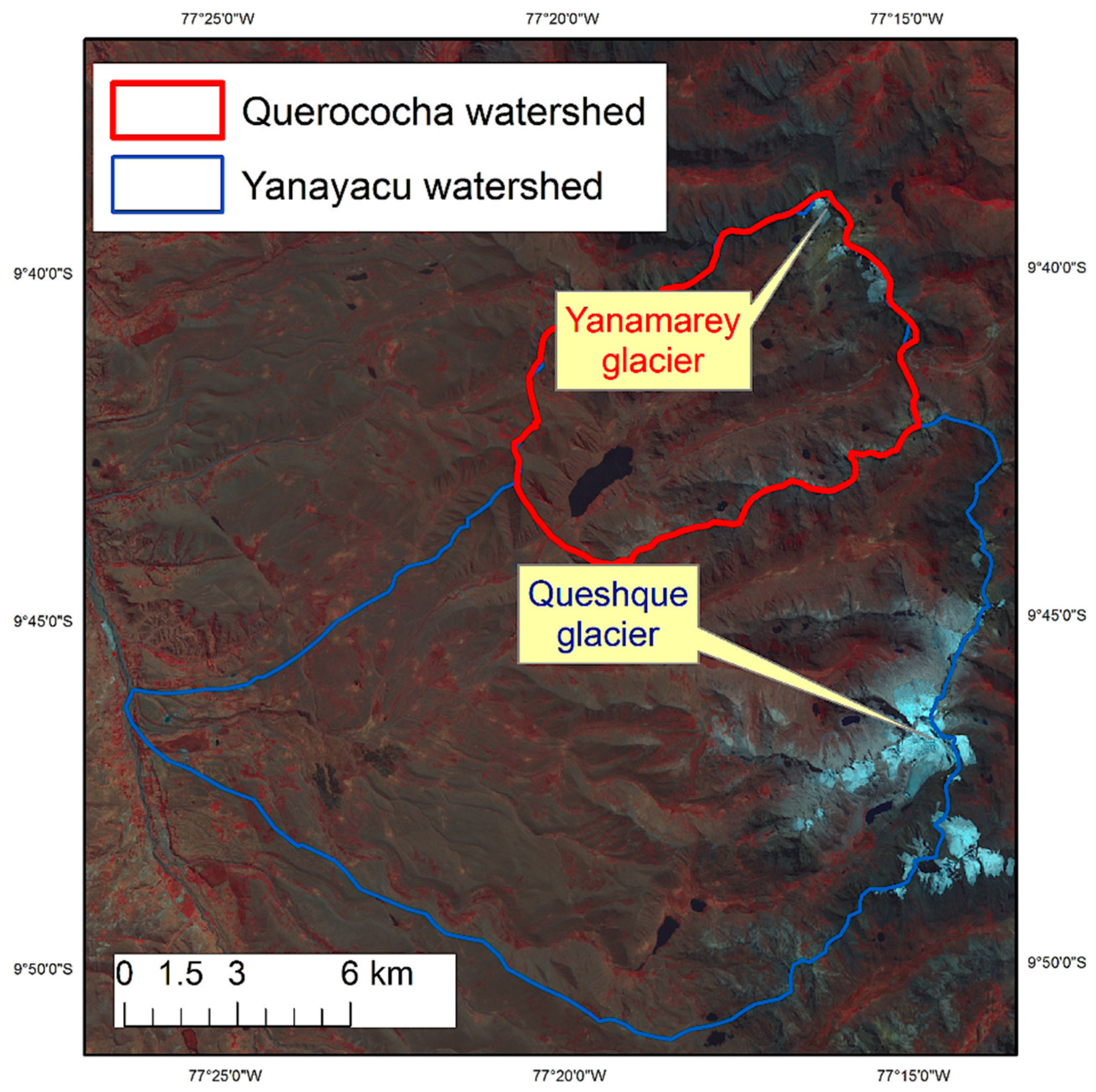
2. Study Site and Geographic Setting

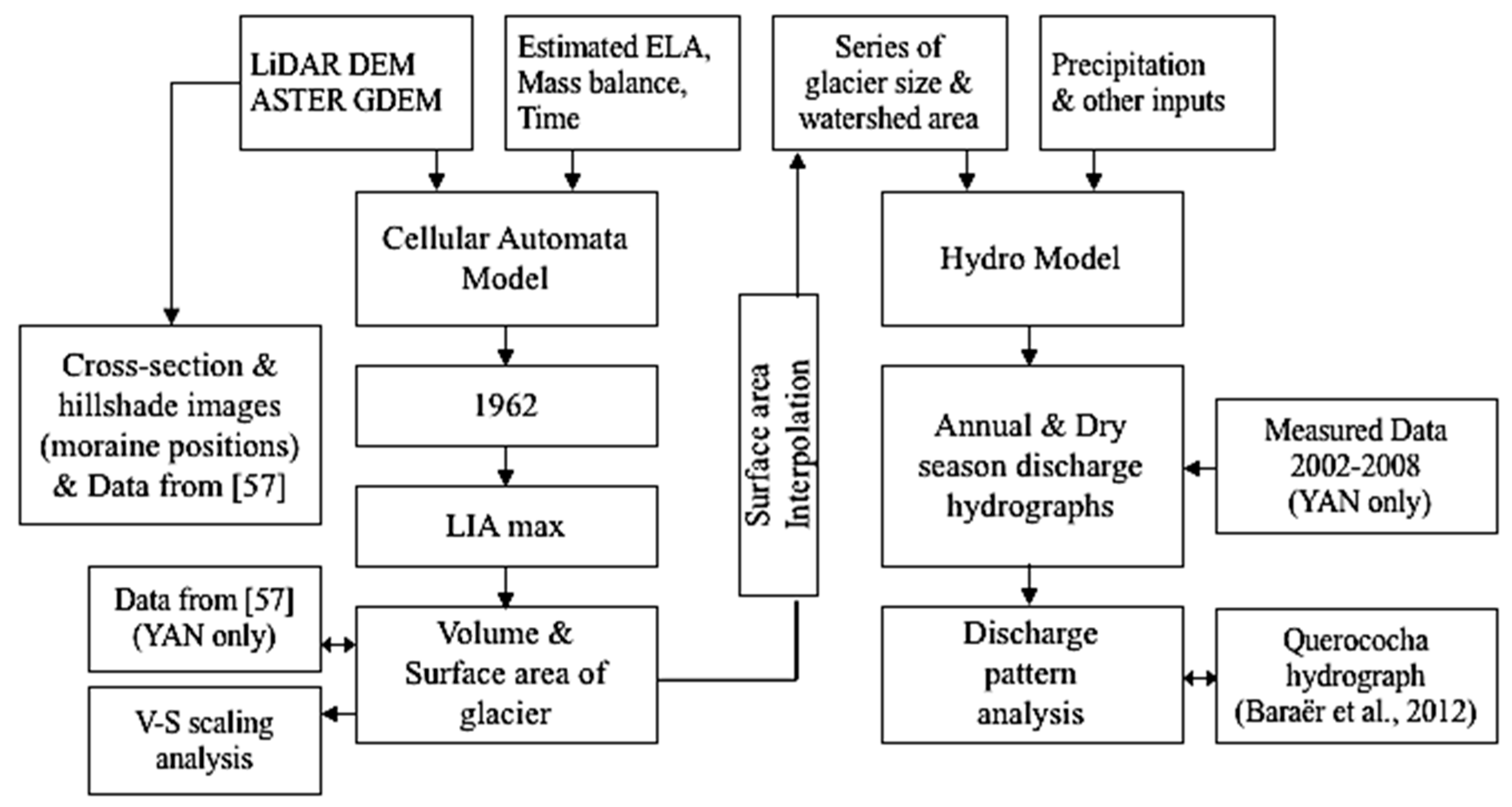
The Cordillera Blanca is the most glacierized range in the tropical region, containing 25% of the world’s tropical glaciers by area. In addition, more than 70% of the world’s tropical glacier area coverage is in Peru [51,52]. It spans 180 km along the South American continent divide between 8° and 10° S latitude, with 27 summits over 6000 m and over 200 peaks over 5000 m in elevation [34,53]. Both the Yanamarey and Queshque main glaciers are the most studied glaciers in terms of hydrology in the Cordillera Blanca, Peruvian Andes, between 9°39′ S–9°52’30’’ S and 77°15′00’’ W (Figure 1). The study area features an outer tropical climate with low thermal seasonality and highly seasonal precipitation. The daily temperature variation is greater than the average annual temperature and the monthly precipitation has a strong seasonality with most precipitation falling between October and April [34,54].

Most glacial meltwater drains into the Santa River, which flows to the Pacific Ocean [1]. The glacier meltwater of the watershed in the Santa River can provide 10 to 20% of the total annual discharge, possibly reaching as much as 40% of the total discharge during the dry season, despite only having <10% glacier coverage in the watershed [3]. The meltwater from the Yanamarey glacier drains within the 64 km² area of the Querococha watershed, which was ~2% glacierized in 2009–2010. Meanwhile, the meltwater from the Queshque main glacier drains into the 277 km² Yanayacu watershed, which was 2.62% glacierized in 2009–2010. As of 2010, the Yanamarey glacier (YAN) had an area of 0.32 km², accounting for 0.50% of the Queroccocha watershed, while the Queshque main glacier (QUE) had an area of 1.37 km², accounting for 0.49% of the Yanayacu watershed.

3. Data and Method

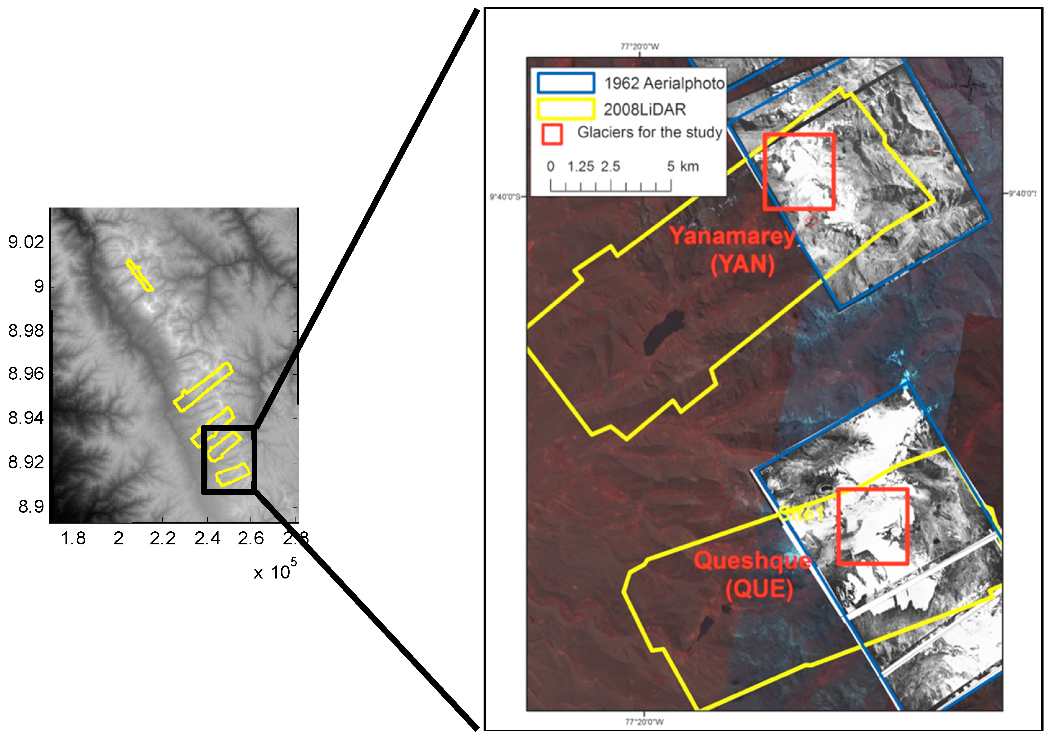
3.1. Remote Sensing Imagery

We computed the rate and magnitude of centennial-scale glacier volume changes for glacier surfaces between the LIA and the modern era, defined by 2008 LiDAR data, as well as 2011 Advanced Spaceborne Thermal Emission and Reflection Radiometer (ASTER) Global Digital Elevation Model Version 2 (GDEM V2) and its imagery. High-resolution airborne LiDAR data were acquired during 2–16 July 2008 (Yellow boxes in Figure 2) and ASTER GDEM V2 was released on 17 October 2011 (covering the entire study area depicted in Figure 2). Also, 1962 aerial photo coverage is represented in the figure by the blue boxes.

For cellular automata modeling, both ASTER GDEM V2 and LiDAR DEMs were used. The dataset was resampled mainly from LiDAR DEM of 10 m and partially from ASTER GDEM V2 of 30 m to fill surface areas where LiDAR DEM data did not cover the glacier valley, to compute paleoglacier flow. ASTER satellite imagery was used for the recent estimates of glacier areas. The absolute vertical accuracy of ASTER GDEM V2 was as small as 8 m (generated from 10–20 ASTER scenes, covering most areas in the Cordillera Blanca) to between 8 and 15 m (produced using five scenes or less over the northern portion of the Cordillera Blanca) [55]. For the model used to reconstruct the glacier volume in this study, DEMs were resampled to a resolution of 100 m to meet the computational requirement of cellular automata modeling.

3.2. Paleoglacier Extent

To check the outputs of the simulation of paleoglacier reconstruction from the cellular automata model, we compared the result with the LIA moraine positions and valley morphology determined from LiDAR shaded relief images created from its DEMs and 1962 aerial photographs. These are valuable sources of information, indicating the previous glacial extent since the LIA [28,31,33,38]. Also, the surveyed data information of YAN [56,57] was used to compare with the model simulation result. We limited the simulation applying the cellular automata model over the two glacier sites (YAN and QUE) due to the visibility of the LIA moraines from the cross-section of LiDAR DEMs and its hillshade images over major glacier valleys for this study. The LIA moraines located down-valley of the target glaciers are readily visible from the cross-section profiles of LiDAR DEMs and 1962 aerial photographs. From the terminus locations of the LIA paleoglaciers, it was possible to estimate the volume and surface area of the paleoglaciers as well as their changes over time.

3.3. Glacier Mass Balance Model: Cellular Automata

We modeled the glacier dynamics 160 years back to the LIA across the landscape using a cellular automata technique in MATLAB version R2016b from MathWorks. The cellular automata model for glacier flow modeling [58] was initially a landscape evolution approach, but a modified version for glacier flow was adopted in this study. A schematic overview of the cellular automata model and a hydrologic water balance model [1] (see Section 3.6 for the hydrology model) is shown in Figure 3.

According to a previous study [58], this approach can examine how glacier dynamics can be simulated. This model is simple because the focus is on a first-order representation of climate and glaciers at the scale of the mountain valley. For modeling, we used simple input parameters such as DEM model, glacier boundary of the initial year, initial year of ELA, initial year of mass balance maximum gradient, time of simulation, and time increment with valley topography.

The model starts from the ice boundary of 2008 glacier polygons and grows the glaciers inversely based on 2008 and 2011 DEMs. The model mimics the accumulation and ablation of snow and ice, as well as its redistribution by glacier motion. The model runs until the time of simulation with the prescribed climate condition. To verify the accuracy of the model, the results of the test run were compared with 1962 glacier polygons over both YAN and QUE. For YAN, an undated LIA maximum, assumed to be around 1850 AD, with a surveyed series of terminus position records (1939, 1948, 1982, 1988) and their longitudinal profiles were available to compare with the model performed [56] (see Figure 4).

3.4. Cellular Automata Model Setup

The landscape was discretized into a regular hexagonal lattice computed from 100-m resolution DEMs for the model requirement. This allows for six degrees of flexibility for particle motion between adjacent cells. The ELA used here as an input parameter was the median glacier altitude for each glacier model run, since the median glacier altitude is an alternative indirect method of depicting the ELAs of glaciers [43]. Furthermore, the ELA began to decrease 1 m per year when the model was run because the ELA increased by about 70 ± 30 m during the 20th century as the glaciers retreated, reaching a 150-m increase in some cases from the 1930s to the end of the 20th century [31]. For a good example, the evolution of the ELA of the Artesonraju over the past centuries shows that the ELA of the glacier around 1850 AD can be easily interpolated to be around 4870–4880 m, from 4860 m in 1800 AD and 4885 m in 1880 AD [31], further increasing to about 5100 ± 50 m during 2000–2005 AD [48]. Since the trend of the Artesonraju is concordant with the general trend, setting the ELA change to 1 m per year for glaciers within the same mountain range for the model would be justified. Meanwhile, the time steps are made to depict mean annual climate conditions. The simulation glacier particles move within the lattice synchronously, at discrete time steps.

The glacier particles representing the water equivalent of snow and ice are added to and removed from the lattice following the rules of precipitation and ablation. The glacial ice motion is considered to be plastic with a yield stress of 1 bar, 100 kPa, including deformation and sliding, which accommodate flux to maintain the basal shear stress, ${\tau }_b$, at the yield stress [59,60].

$${\tau }_b=\rho gh sin\alpha \approx 1 bar,$$

(1)

where $\rho$= density, $g$= acceleration due to gravity, $h$= ice thickness, and $sin\alpha$= ice surface slope. Values of ${\tau }_b$are normally between 50 and 150 kPa (100 kPa = 1 bar). The flux determines the velocity and geometry of glaciers. Plasticity is a widely applied simplification in glacier flow modeling [60] and holds to the first order provided that along-glacier shear is the dominant mode of deformation. A large body of observational and analytical evidence supports this assumption [20,60], including in situ measurements of the full strain rate tensor in a valley glacier [61].

When the model runs, any ice thickness causing stress exceeding 1 bar will flow to the lower adjacent cell. Although the model does not reconstruct ice flow perfectly, the results predict the general LIA glacier extent [58]. The mass balance was assumed to be constant the accumulation area, while the value was set to decrease at a constant rate of 6 m/year/km of altitude in the ablation area based on the balance gradient [56] and maximum accumulation of 1 m/year. The parameters for the cellular automata model for YAN and QUE are listed in

Table 1. Input parameters for the cellular automata model employed in this study.

Parameters	YAN	QUE
Median height (m) from DEM	4898	5057
Equilibrium Line Altitude (ELA) for model (m)	4780	4950
Net balance in ablation (103 kg m−2 year−1)	6	6
Max mass balance (103 kg m−2 year−1)	1	1
Total time (year) (test: 2011 to 1962)	49	49
Total time (year) (2011 to 1850)	161	161

YAN: Yanamarey glacier, QUE: Queshque main glacier.

.

First, the test version of the cellular automata model (almost 50 years; 2011 to 1962) was performed to evaluate the model by comparing 1962 glacier polygons from aerial photographs available for target glacier valleys. After these tests were completed, the LIA paleoglacier modeling was conducted for both the YAN and QUE sites. Then, we performed the modeling of the LIA glaciers retrospect over 161 years (younger and minor advances: 1850 AD) [28,31,38].

To check the ability of the model to accurately simulate paleoglaciers, the simulation results were compared with surveyed records from previous research [57]. The headwall-to-terminus distance, the elevation of the terminus position, the surface area, and the volume of all reconstructed information of the YAN site over different years were compared with the available measurement data [57].

3.5. Volume and Surface Area (V-S) Scaling from the Model

After the simulation to reconstruct paleoglaciers through the LIA maximum for YAN and QUE was achieved, the volume and surface (V-S) scaling for individual glaciers was performed. The volume (V) of any individual glacier or ice cap is related to its surface area (S) by a simple power law relationship expressed with a scaling coefficient ($C_0$) and a scaling exponent ($C_1$) that depends on glacier type, both empirically computed from the measured V and S [19,20] as follows:

$$V=C_0\cdot S^{C_1},$$

(2)

where the unit of $V$ is 10⁶ m³ and that of $S$ is 10⁶ m². Observations of a wide range of glaciers mostly located in mid and high latitudes gave values of 28.5 and 1.36 for $C_0$ and $C_1$, respectively [19,20,21]. This value of $C_1$agrees with observations from References [20,62,63].

Based on six glaciers, including YAN and QUE, in the Cordillera Blanca [64], Equation (2) becomes:

$$V=48.032\cdot S^{1.275}.$$

(3)

The uncertainty of the V-S scaling of Equation (3) based on the principle of error propagation [64,65] shows that the magnitude of error of V-S scaling is approximately 25% of the computed volume (V). Equation (3) of the V-S scaling from six glaciers in the Cordillera Blanca [64] was compared with the scaling factors from the V-S scaling of YAN and QUE obtained from the reconstructed surface area and volume as well as the change in surface area and volume. Also, the volume difference of YAN between the literature and the results from the cellular automata model presented here was taken as an uncertainty of the reconstruction using the cellular automata model.

3.6. Hydrology Model

We also performed an experimental approach to model changes in glacial meltwater using a water balance model to see if the historical mountain glacial hydrology regime could be reconstructed back to the LIA maximum. This enabled us to analyze the long-term trend of glacial meltwater discharge as well as the impact of the recession of glaciers. The schematic overview of the water balance model with the cellular automata model is shown in Figure 3. This water balance model is a relatively simple approach [1], which can evaluate both historical and recent time series of the discharge of selective watersheds in the Cordillera Blanca as well as calculate discharge hydrographs based on glacier retreat sequences. The water balance model for the yearly discharge (Q_n) [1] can be expressed as follows:

Q_n= (ΔV_gl + pp·A_gl)·d_melt + (A_T − A_gl) · (pp − et_ngl) − ET_rl,

(4)

where ΔV_gl is the interannual change in glacier volume in water equivalent, pp is the average depth of precipitation received, et_nglis the non-glacierized evapotranspiration per unit area, d_melt is the fraction of annually ablated ice (snow and firn included) that is not lost by sublimation, and finally A_T and A_gl are the total watershed area and glacierized areas, respectively. The dry season discharge (Q_dn) can be expressed as follows:

Q_dn = (ΔV_gl + pp·A_gl)·αd’_melt + (A_T − A_gl) · q_ngl − ET_rl,

(5)

where α is defined as the fraction of annual ablation that occurs during July and August, d’_melt is used instead of d_melt, and q_ngl is the net slow-flow dry season specific discharge, which accounts for the water released from groundwater minus the specific transpiration.

The major input parameters for the model to create synthetic hydrographs are the initial glacierized surface area, the watershed area, and the annual average precipitation. The LIA paleoglacier maximum extent of the mid-19th century (around 1850 AD) was estimated from both the cellular automata model and the LIA moraine positions and was then used as an input parameter to determine the initial glacier surface area. As the model requires a continuous time series of glacier areas over the study period, the outputs of the cellular automata model for YAN were interpolated using pattern assimilation from a published description of regional glacier area fluctuation over the last 150 years [40]; the glacier front position data recorded in 1948 and a time series from 1976 to 2006 by the Autoridad Nacional del Agua (ANA) del Peru; and the 1962 aerial photo-based estimates [64] with recent estimates of 2001–2008 obtained from ASTER satellite imagery [64]. The model assumes that the path of glacier surface area change was similar to that of glacier front retreat. The retreat sequence pattern implies that glaciers were generally retreating slowly from 1850 to 1920 [40]. This period was followed by a marked advance from 1920 to 1930, leading to glacier surface areas almost equal to those of 1850. The period between 1930 and 1945 was characterized by a strong mass wasting from the glaciers, which slowed after 1945. Both glacier surface area time series were extrapolated until 2050 to provide estimations of how stream discharge may change as the glaciers continue to retreat. The projection of glacier surface area was simply based on a quadratic extrapolation from the glacier surface area of 2001–2009. The times series of change in surface area were substituted for the annual glacier retreat rate of surface area with a linear interpolation in the model. A similar method was used to create the QUE surface area time series using the YAN surface area fluctuation pattern as a model.

Precipitation yearly average was kept constant at 1850 mm per year for the entire studied period in the model. This was justified by the absence of a regional trend in precipitation over the period of record [1]. Using a fixed precipitation value for the simulation allowed for the removal of noise of the interannual natural variation, which would have affected the discharge simulation. Therefore, the fixed precipitation parameter allowed the model to produce discharge time series that fluctuate only from glacier retreat. This benefit was obtained at the expense of the year-to-year representative of the model. Consequently, only discharge trends can be interpreted from the model output and the year-to-year variations cannot be considered to match the reality. The value of 1850 mm per year was adjusted from the historical precipitation record from two meteorological stations of 1981–1999 and 2001–2008 located near YAN in the Querococha watershed [66]. Other model parameters were adjusted from those that were applied to the Querococha watershed, which hosts YAN (Figure 1), in a previous study [1] based on the yearly and the dry season discharges recorded at a discharge station situated at the outlet of the YAN proglacial lake. This was achieved by targeting a yearly mean discharge difference between the simulated and observed discharges of less than 5% for the data available from 2002 to 2007. Considering QUE, which has the same orientation as YAN and is located within 15 km, we kept the model parameters tuned for YAN since there is no gauge system installed at the Yanayacu watershed, which hosts QUE. The parameterized model result was used to generate time series of the yearly average discharge (Q) and the yearly dry season discharge (Q_dry) based on precipitation, the time series of the glacier surface area, and the surface area of the watershed.

4. Results and Discussion

4.1. Cellular Automata Model

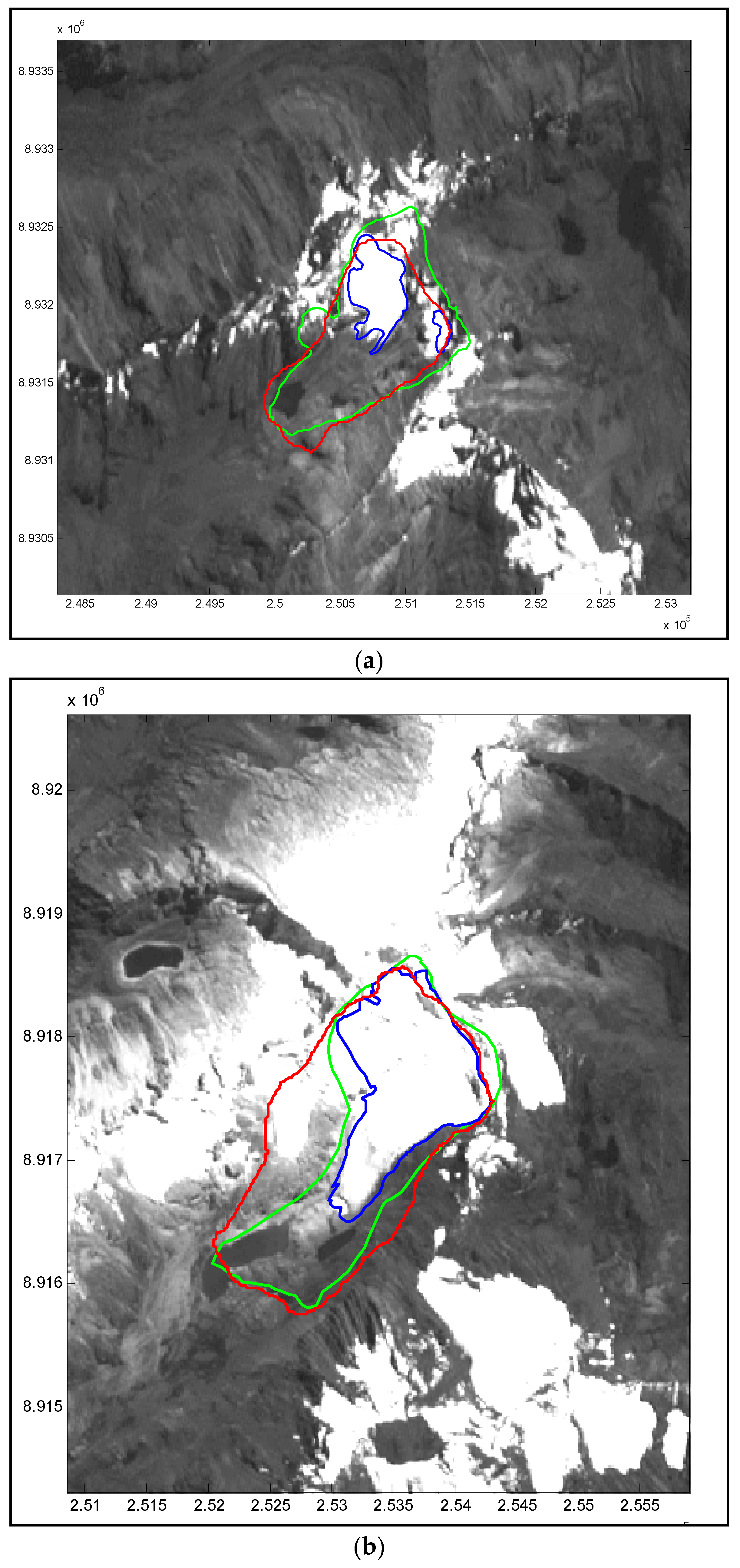
4.1.1. Modeling Test: 50 Years Back (2011 through 1962)

To evaluate the model, first we performed a test run from the 2008 glacier polygons for YAN and QUE extracted using 2008 ASTER images (almost 50 years; 2011 to 1962) and compared the results with the 1962 glacier polygon extracted from the 1962 aerial photographs (Figure 5). All three different polygons of the test results of the modeled glacier boundaries (shown in red) of YAN and QUE, 1962 glacier polygons (shown in green), and 2008 glacier polygons (shown in blue) are displayed in 2D (Figure 5).

The results in Figure 5 show that the modeled glacier terminus positions agree with the positions based on the pictorial representation from 1962 aerial photographs. For QUE, the modeled glacier coverage is wider in the valley than the actual 1962 glacier extent. This may be because the cellular automata model is sensitive to the shape of the glacier valley and topography. If the shape of the valley is wide at the initial stage of the model run, then the output of the model gives a broader surface area, and this may affect the V-S relationship.

Through repeated model runs over both glaciers, we confirmed ELAs of 4780 m for YAN, 4950 m for QUE, and a net balance gradient of 6 m/year/1 km. For the comparison with the 1939 AD field record for YAN [57], we ran the model through 1939 AD. Based on parameters from the illustrated results of the test run, we performed the modeling of the LIA glaciers retrospectively up to 161 years (younger advance: 1780–1880 AD, LIA maximum in 1850 AD) [28,31,38].

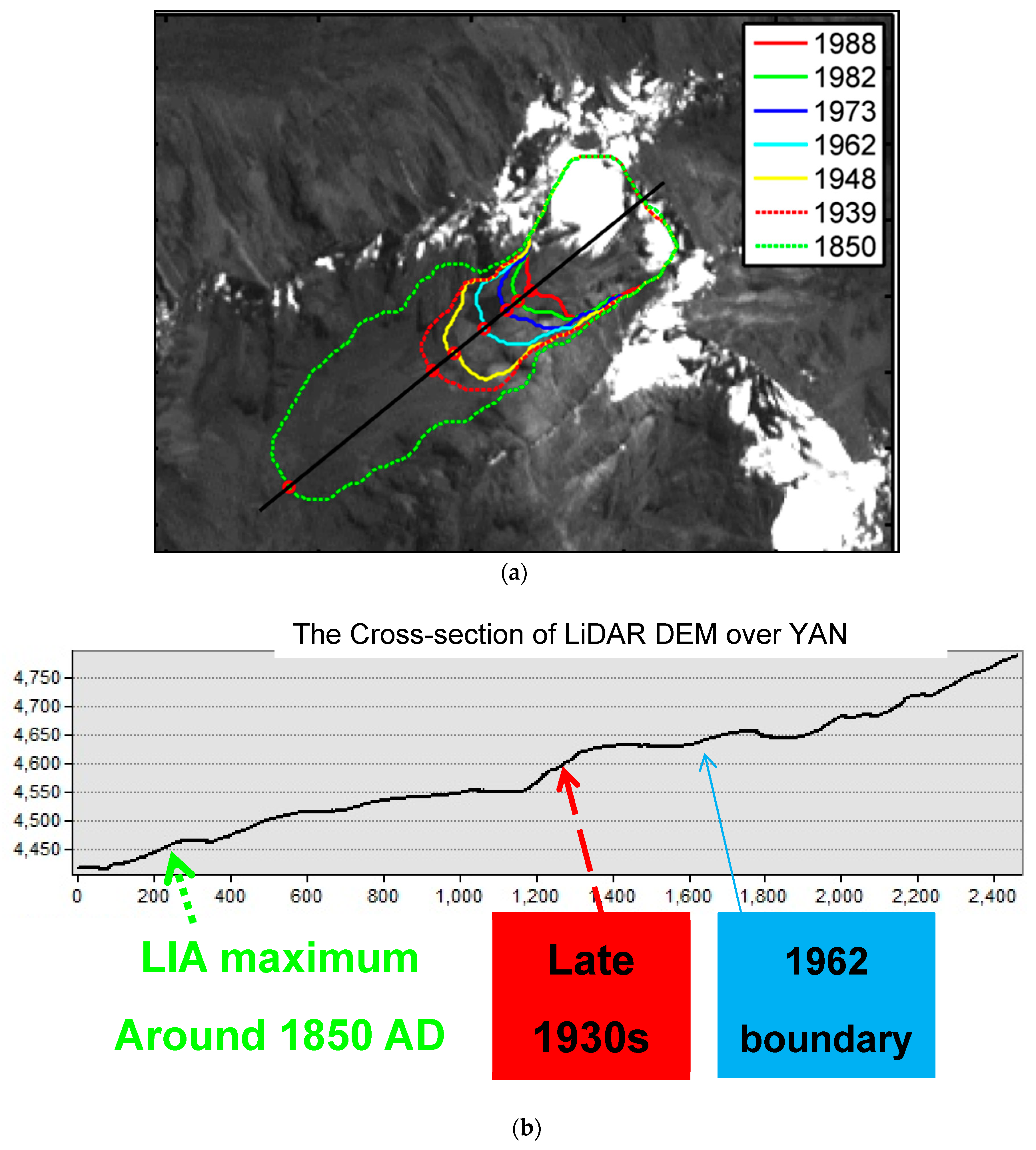
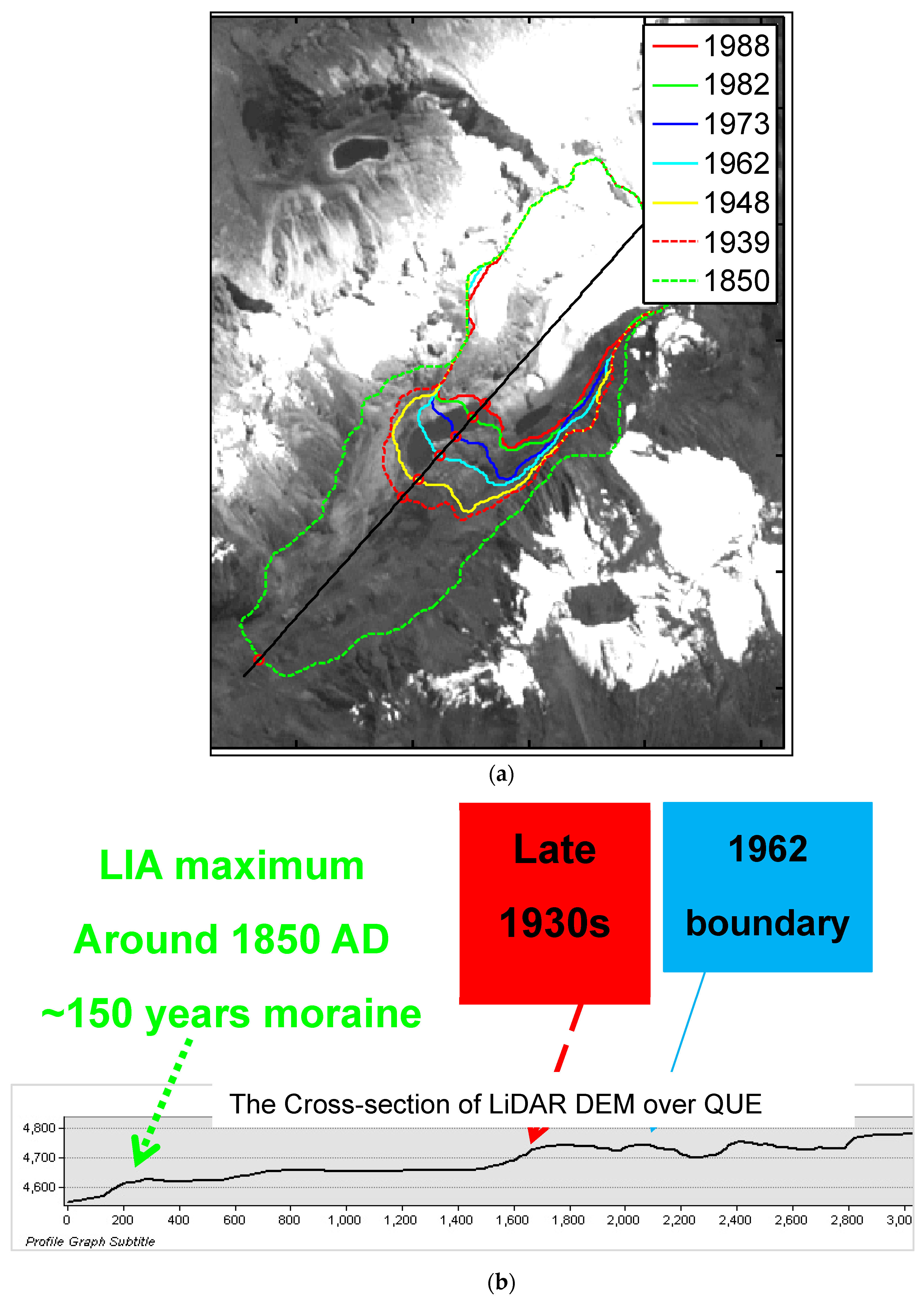
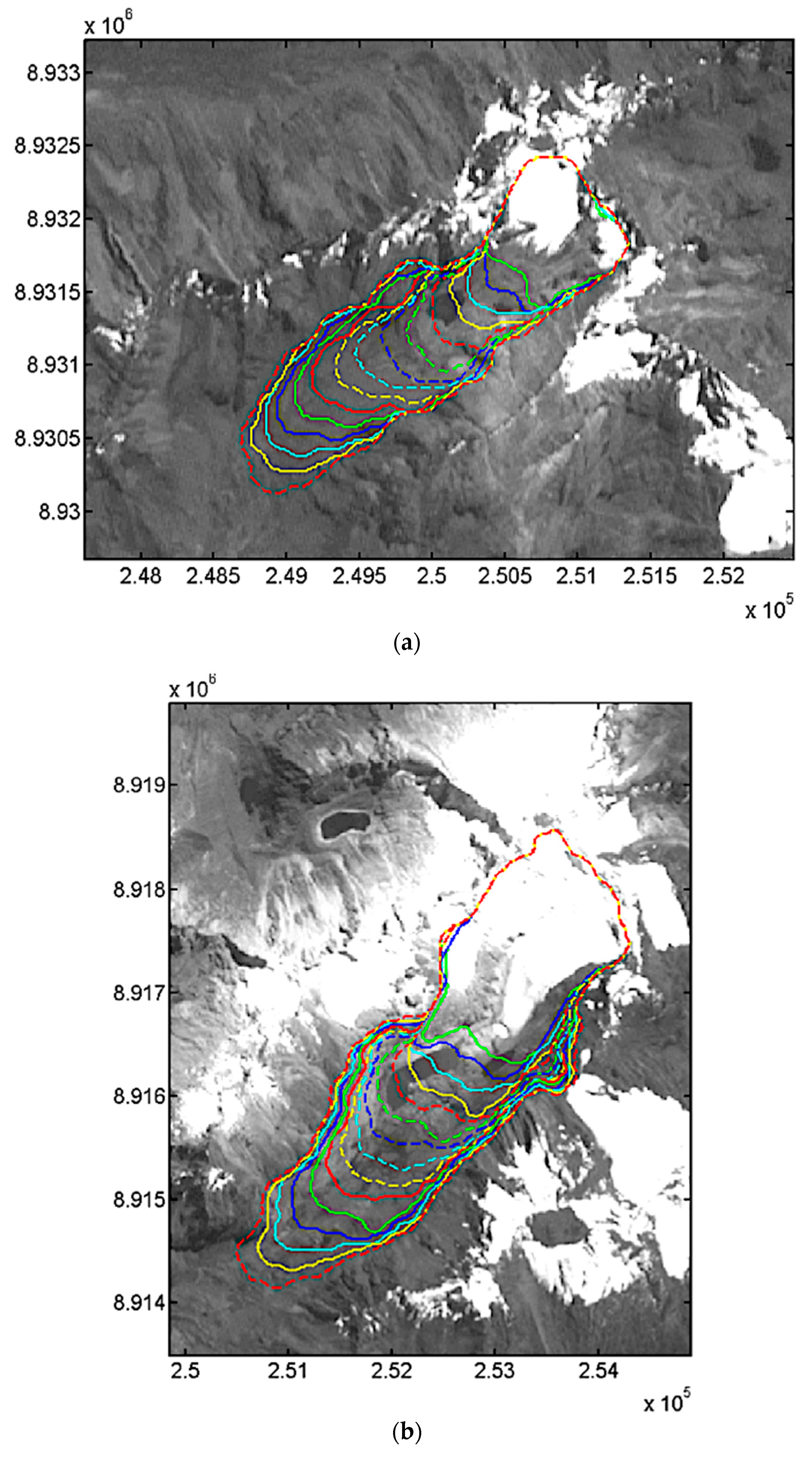
4.1.2. Modeling through LIA Maximum (1850 AD)

Starting from the 2008 terminus achieved from 2008 polygons, the cellular automata model simulated until the LIA maximum for both YAN and QUE with an ELA decrease of 1 m per year. While the model was simulating, the new ELA was computed from the new glacier boundary and the new updated ELA in retrospect to 150 years, indicating an LIA maximum ELA 150 m lower than the present ELA. The pictorial result of the simulation shows the evolution of YAN over the period studied (See Figure 6a).

The comparison of the length, surface area, and volume of YAN (headwall to terminus) between the model and that reported in Reference [57] is described in Section 4.2. The simulation output and the measurement data show good agreement [57]. Although there is no reference for QUE, the simulation was performed based on the retrospect time series of 1988–1939, the same as YAN, as shown in Figure 7, and revealed that the modeled glacier terminus positions agree well with the moraine positions obtained from the cross-section of the LiDAR DEM. Figure 8 shows the series of reconstructed paleoglacier boundaries over a 10-year interval.

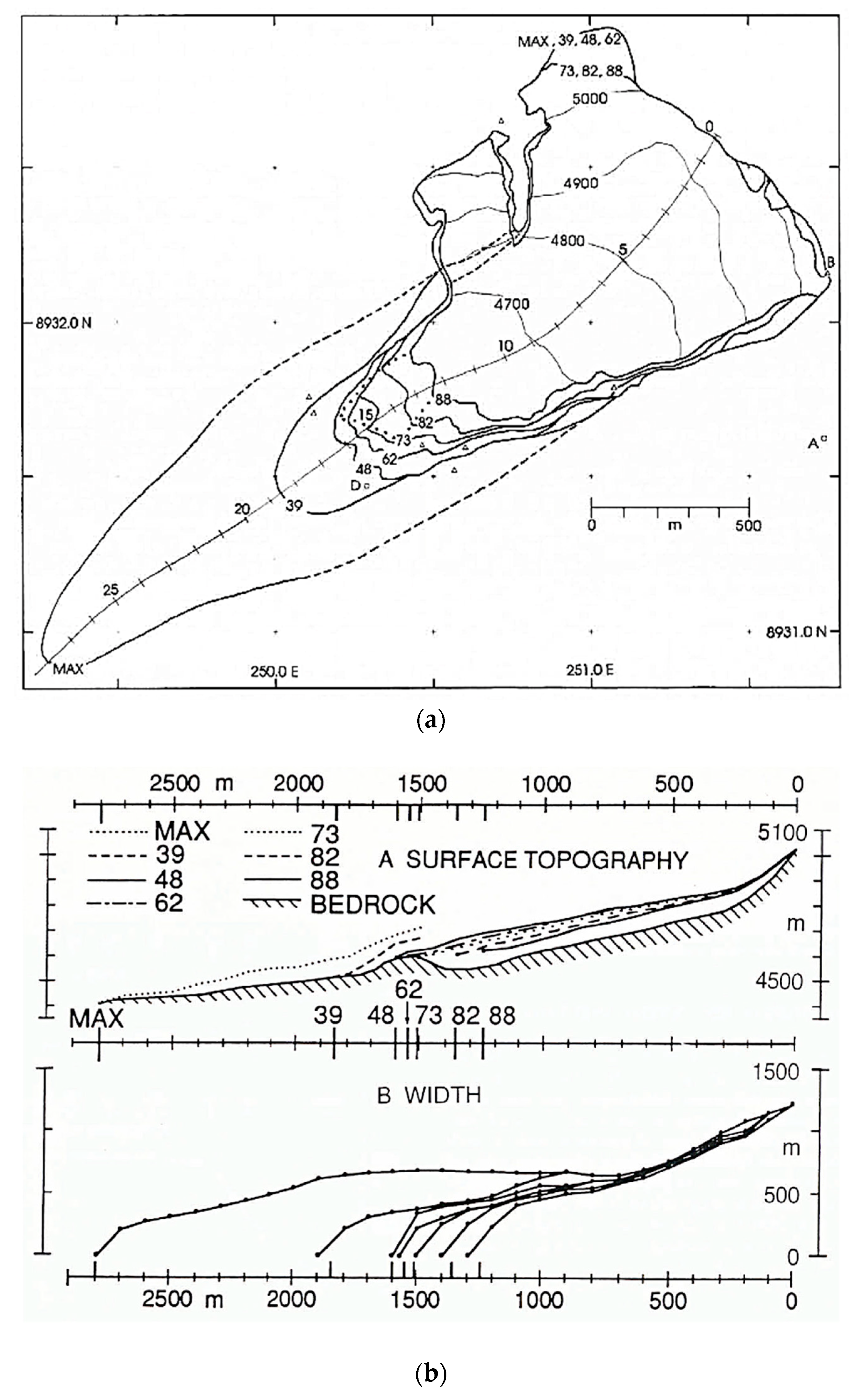
4.2. Model vs. Previous Research on YAN

How well does the model reconstruct the glacier? To assess the model’s performance of YAN simulation, the outputs were compared with surveyed data [57]. Although these measurements are short-term and intermittent, they are enough to compare on a year-to-year basis (

Table 2. The comparison between model outputs and measurement data from previous research [57]. H&A is from the surveyed data from [57].

	Distance from Headwall to Terminus (m)			Terminus Elevation (m)		Surface Area (106m2)		Volume (106m3)
Year	Model	H&A	Diff.	Model	H&A	Model	H&A	Model	H&A
1988	991.65	1250	258.35	4631.3	4630	0.86	0.8	32.29	25
1982	1098.28	1350	251.72	4625.92	4600	0.91	0.87	35.04	32
1973	1268.88	1500	231.12	4618.86	4595	0.97	0.95	38.43	-
1962	1432.62	1550	117.38	4624.55	4600	1.05	1.02	43.09	-
1948	1695.40	1600	−95.40	4600	4590	1.20	1.0	52.27	54
1939	1855.34	1850	−5.34	4530.34	4520	1.22	1.2	59.99	-
1850	2991.60	2800	−191.60	4348.13	4420	1.73	1.7	88.71	89

).

Generally, the modeled glacier terminus positions agree with the measured positions [57]. The model output shows that the difference in distance between the model and the reference is about 117 m in 1962 AD, decreasing to 5.34 m in 1939 AD. For 1850 AD, the terminus position from the model simulation is 191.60 m longer than the position of the reference. However, the surface area and volume between the two show results indicating that there are no big differences between the model and reference (Table 2).

The cellular automata model with simple parameters succeeded in simulating the extent of the LIA maximum paleoglacier over the YAN and QUE valleys, although the model did not mimic the ice flow exactly. The results were based on constant climate parameters except for the ELA setting, while glaciers in the real world exist under variable climate conditions. We presumed that the ELAs were within a few tens of meters of the modeled value, although we do not have any field evidence to back this up. Although setting the ELA to decrease by 1 m per year for the model may not be realistic for the beginning years retrospectively, it may be valid for a long-term model simulation. Therefore, the simulation result should represent conditions averaged over centuries. Also, the length and the width of the simulated glaciers may be sensitive to the complex elevation distribution of both surface area and slope. However, long-term mass balance data do not exist for broader mountain ranges in the Cordillera Blanca and only cumulative values are available for a few glaciers without time series [56,57,67,68,69]. Also, there are limited numbers of chronology studies for the study area, and those that exist are focused more on millennial scales (Last Glacial Maximum; LGM) [29,30,70,71,72]. This limits the possibility of comparing our regional, long-term model to ground truth over the entire range. Moreover, the results of the model simulation were based on constant climate parameters, while glaciers in the real world exist under non-stationary climate conditions.

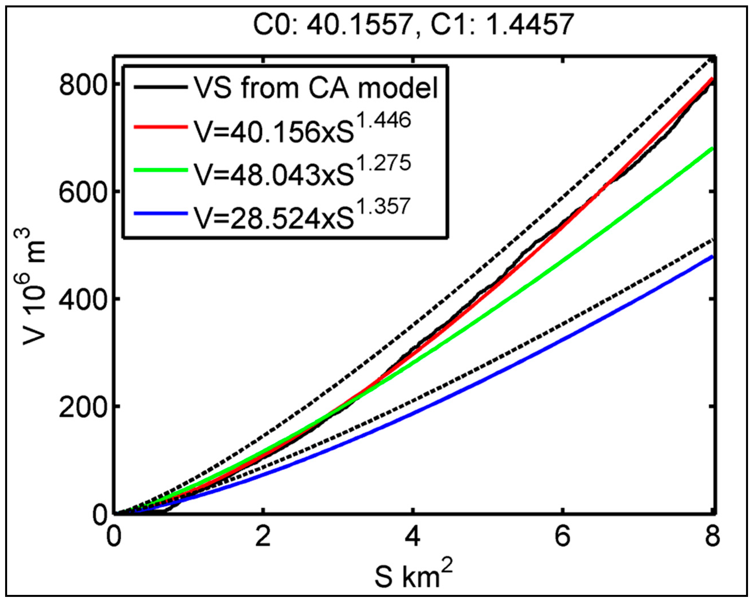
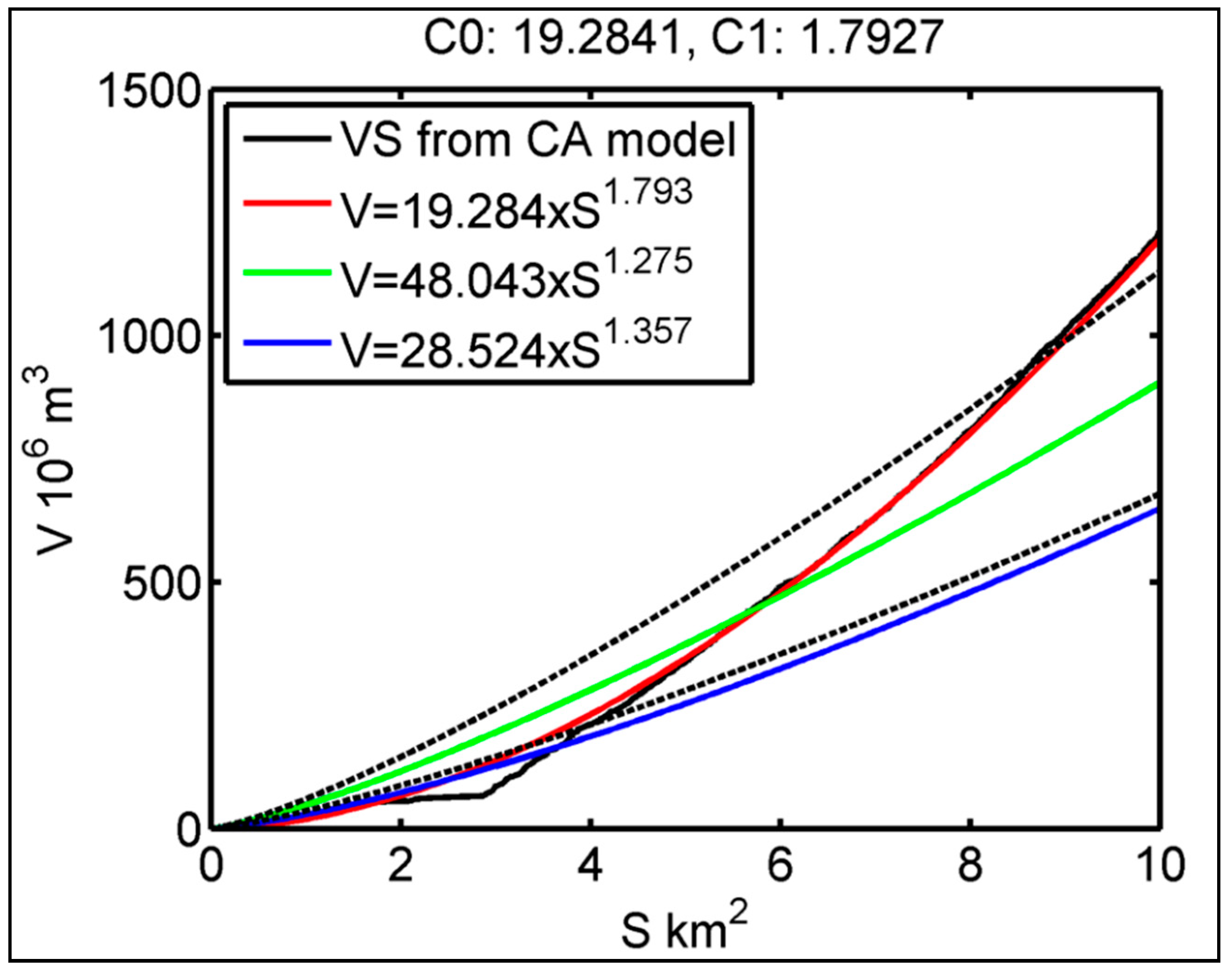
4.3. Volume Reconstruction from the Model vs. V-S Scaling Fit

4.3.1. The V-S Scaling of YAN from the Cellular Automata Model

Based on the reconstructed surface area ($S$) and its volume (V), Equation (2) for YAN can be written as follows and is shown below in Figure 8:

$$V=40.156\cdot S^{1.446}.$$

(6)

The V-S scaling over YAN from the simulation shows $C_0=40.156 \mathrm{and} C_1=1.446$. Since the V-S scaling relationship over glaciers in the Cordillera Blanca [64], including YAN, shows that $C_0=48.043 \mathrm{and} C_1=1.275$, the differences in volume between the V-S scaling from six glaciers in the Cordillera Blanca, including YAN, and the V-S scaling generated from the cellular automata model of YAN were 8.20% in 1850 AD (size of 1.73 km²), 14.33% in 1962 AD (size of 1.16 km²), and 22.15% in 2001 AD (size of 0.66 km²), while the difference in volume between the V-S scaling of YAN from the cellular automata model and that from Chen and Ohmura (1990) ranged from 26 to 32% (

Table 3. Difference in the V-S scaling of YAN between the cellular automata model and six glaciers in the Cordillera Blanca [19,64].

Year	Size (km2)	Volume from V-S Scaling CA (106m3)	Volume from V-S Scaling CB6 (106m3)	Volume from V-S Scaling C&O (106m3)	Volume Diff. (CB6 vs. CA) (%)	Volume Diff. (CA vs. C&O) (%)	Volume Diff. (CB6 vs. C&O) (%)
1850	1.73	88.71	96.64	60.01	8.20	32.35	37.90
1962	1.16	49.46	57.73	34.68	14.33	29.88	39.93
2001	0.66	22.02	28.28	16.23	22.15	26.29	42.62

CA: cellular automata model; CB6: six glaciers in the Cordillera Blanca [64]; C&O: from Reference [19].

).

The approach using the cellular automata model to reconstruct paleoglaciers and their V-S scaling works well for YAN because the model shows that the volume estimation achieves a similar range (8.20%) when the glacier reached the LIA maximum in 1850 AD (Table 3).

Also, we can verify the error estimation of the V-S scaling in Figure 9. Based on the 25% error range (six glaciers in the Cordillera Blanca) calculated from the error propagation [64] (black dotted line shown in Figure 9), it can be observed that the V-S scaling estimated from the cellular automata model of YAN it is very similar to the V-S scaling calculated from the data of six glaciers in the Cordillera Blanca. Moreover, the fitting seems to be in a good range until the surface area does not exceed 4 km². Although the V-S scaling of the cellular automata is always within the 25% error range in the reconstruction simulation, the volume estimation should work for glaciers smaller than 8 km² [64].

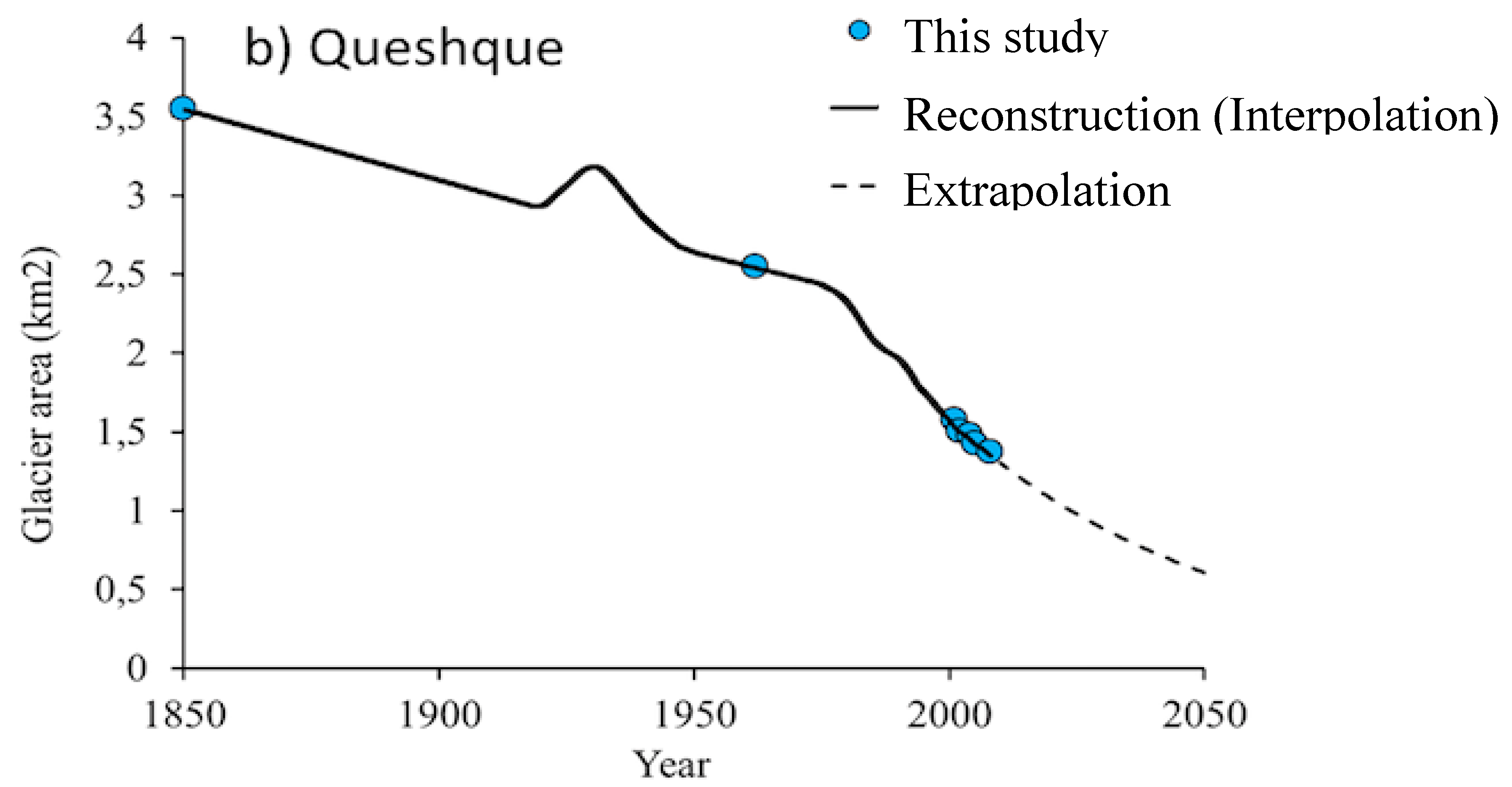
4.3.2. The V-S Scaling of QUE from the Cellular Automata (CA) Model

Based on the reconstructed surface area ($S$) and its volume (V), Equation (2) for QUE can be written as follows and is shown below in Figure 10:

$$V=19.284\cdot S^{1.793}$$

(7)

The V-S scaling over QUE from the simulation using the cellular automata (CA) model shows $C_0=19.284 \mathrm{and} C_1=1.793$. Since the V-S scaling relationship over the glaciers in the Cordillera Blanca [64], including YAN, shows that $C_0=48.043 \mathrm{and} C_1=1.275$, the differences in volume between the V-S scaling generated from the CA model of QUE and that calculated from the data of six glaciers in the Cordillera Blanca, including QUE, were 22.63% in 1850 AD (size of 3.55 km²), 34.82% in 1962 AD (size of 2.55 km²), and 49.29% in 2001 AD (size of 1.57 km²) (

Table 4. Difference in the V-S scaling of QUE between the CA model and six glaciers in the Cordillera Blanca [19,64].

Year	Size (km2)	Volume from V-S Scaling CA (106m3)	Volume from V-S Scaling CB6 (106m3)	Volume from V-S Scaling C&O (106m3)	Volume Diff. (CB6 vs. CA) (%)	Volume Diff. (CA vs. C&O) (%)	Volume Diff. (CB6 vs. C&O) (%)
1850	3.55	186.96	241.64	159.17	22.63	14.86	34.13
1962	2.55	103.3	158.47	101.59	34.82	1.65	35.89
2001	1.57	43.3	85.39	52.61	49.29	−21.50	38.39

CA: cellular automata model; CB6: six glaciers in the Cordillera Blanca [64]; C&O: from Reference [19].

). While the simulation of QUE showed that the glacier surface area grows unrealistically wide at the initial stage (Figure 5b and Figure 7b), the volume estimation of the V-S scaling from the model was 21% lower than that in a previous study [19]. This also confirms that the CA model is sensitive to the shape of the glacier valley and its topography.

Nevertheless, from the error estimation of V-S scaling with the 25% error range (black dotted line shown in Figure 9), the V-S scaling estimated from the CA model of QUE exhibited fitting in a good range until the surface area (S) does not exceed 6 km² (Figure 10).

From the results, the V-S scaling using the reconstruction simulation from the CA model showed that the absolute error of the volume estimation increases with the size of the glacier; therefore, the volume of larger glaciers should be individually estimated. Again, the shape of the glacier valley and its topography should be considered for the error propagation of the CA model.

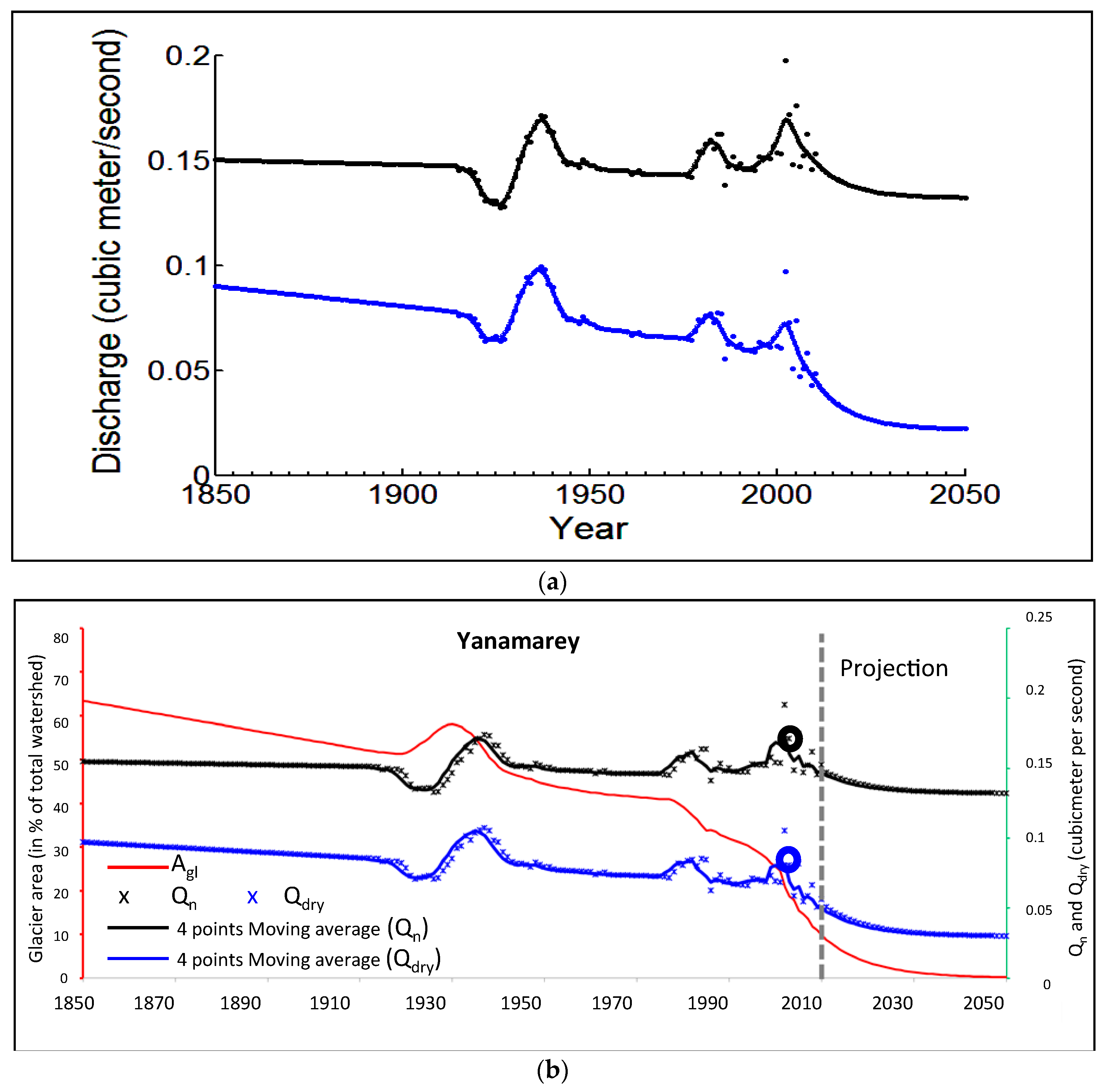
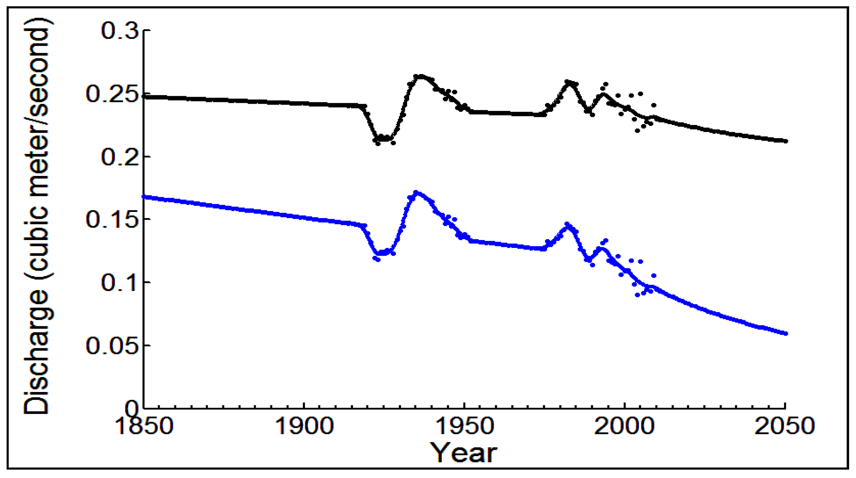
4.4. Hydrology Model

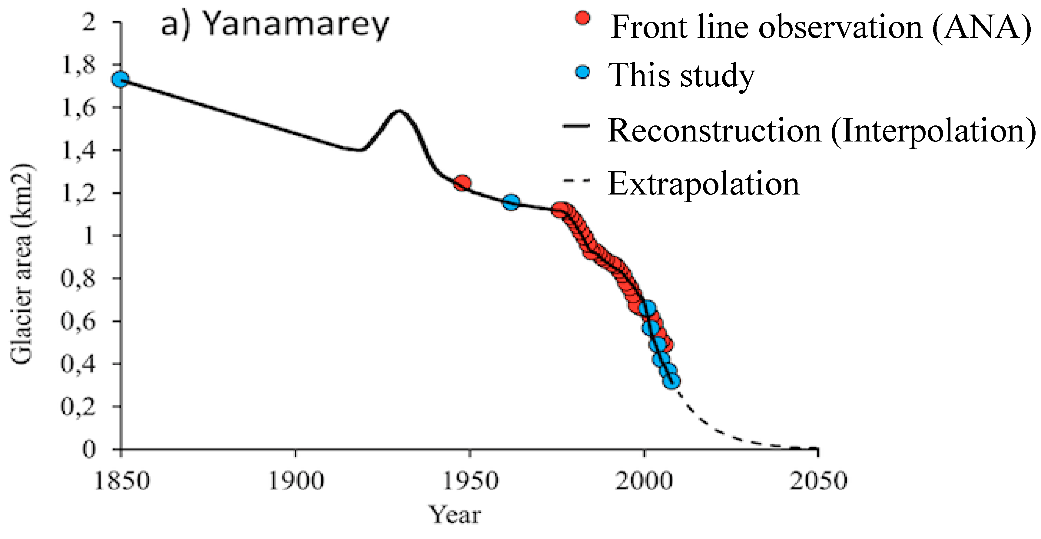
4.4.1. The Yanamarey Glacier (YAN)

YAN showed an average surface area loss of 72.62% with an average loss of 1.58% per year during the period of 1962–2008 [64], while the Querococha watershed showed the fastest glacial area reduction with an average loss of 1.1% per year between 1953 and 2009 [1]. Since there was a temporary glacier advance during the 1920s [40], we applied the glacial re-advance and the retreat as inputs for the model. From 1962 to the mid-1970s, the model showed that YAN started a gradual retreat with a smooth decline, followed by a dramatic decrease in surface area from the mid-1970s to the late 1990s. This was also proven by YAN length data measured from ANA del Peru [73] (see Figure 11).

The model results for YAN gave two synthetic hydrographs of yearly discharge (black) and discharge in the dry season (blue), as well as the change in surface area of the glacier (red) (Figure 12).

From the perspective of discharge, the model results showed that there were three major peaks for both yearly (Q in black) and dry season (Q_dry in blue) discharges in the late 1930s, 1980s, and early 2000s, as depicted in Figure 12a. When YAN re-advanced in the 1920s, the discharge pattern showed a downward trend due to the extra frozen water storage that did not release water. From the late 1970s to the mid-1980s, the model showed a second peak for both the yearly discharge (Q) and the annual dry season discharge (Q_dry) to match the start of the accelerated glacier retreat. This pattern could also be observed at the watershed level, where a clear acceleration in the dry season average discharge was calculated from daily data in the Querococha watershed from the early 1960s, followed by a dominant decrease after the early 1980s [1]. In the early 2000s, another peak in discharge was observed, lasting for 4–5 years while the glacial retreat was exceptional and ice reservoir decreased. We also marked the yearly averaged measured discharge dataset of YAN (measured during 2002–2008 AD) to compare the model and the actual dataset (shown in two large empty circles (black and blue) located around the late 2000s), as shown in Figure 12b. Overall, the model results were close to the measured annual and dry season discharge data.

During the whole studied time period, from 1850 to 2050 AD, the yearly discharge (Q) did not change much (around 13.3% reduction; 0.15 m³s⁻¹ to 0.13 m³s⁻¹); however, the dry season discharge (Q_dry) decreased significantly along with the recession of glacier surface area (over 77.8% reduction; 0.09 m³ s⁻¹ to 0.02 m³ s⁻¹). Based on the changes in the surface area data [73] and the findings of this study, the demise of YAN will be unavoidable after 2040.

4.4.2. The Queshque Glacier (QUE)

After the interpolation of glacier surface area available for this study, the pattern showed a change in the surface area of QUE from 1850 AD to the 1980s, which was similar to that of YAN. Subsequently, the surface area of QUE decreased in a more gradual fashion through the 2000s (Figure 13).

The model results of QUE showed that synthetic hydrographs of both yearly and dry season discharge have two distinct peaks, but the response to the recent retreat acceleration of QUE was different. QUE does not show a clear separation between the two last peaks, where YAN may have experienced the most dramatic glacier retreat impact on discharge at the beginning of the 21st century (Figure 14). Also, we found that the discharge of the dry season (Q_dry) is predicted to decrease as the surface area of the glacier becomes smaller. Likewise, from YAN, during the whole studied time period from 1850 AD to 2050 AD, the yearly discharge (Q) does not change much (around 16% reduction; 0.25 m³ s⁻¹ to 0.21 m³ s⁻¹), while the dry season discharge (Q_dry) is decreased significantly along with the recession of glacier surface area (over 64.7% reduction; 0.17m³ s⁻¹ to 0.06 m³ s⁻¹).

The results of YAN and QUE both showed a dramatic decline in water availability during this century, as small glaciers in the Cordillera Blanca will disappear and precipitation becomes the only water resource [74]. However, the overall annual discharge may not vary much due to possible increased runoff during the wet season. Another study also showed that the annual discharge may not change significantly but seasonality will be greatly intensified in one catchment in the Cordillera Blanca [6]. Climate simulations based on four different Intergovernmental Panel on Climate Change (IPCC) emission climate scenarios show the same prediction over the Llanganuco catchment as is the case of YAN in the Querococha catchment—that total annual runoff remains almost unchanged for all model runs due to much more direct runoff, which compensates for reduced glacier melt under the higher amount of total precipitation. However, future water management will be challenged by a much greater decrease of low runoff from all scenarios of model runs for the dry season in the Cordillera Blanca, Peru [6].

The reconstructed initial glacierized area parameter from the CA model, the surface area information from previous research in the middle of the model period [1], and the glacierized area calculated from ASTER imagery from 2001–2008 help fill in the data gaps and improve the analysis to link glacial retreat and runoff discharge. Observing multiple peaks in mean annual and dry season discharge hydrographs from the results of this study shown in both glacier catchments is the first case of glacier meltwater runoff models implemented in the same mountain range [75]. Moreover, this case confirms that the inclusion of more datasets of glacierized area as input parameters will improve the assessment of past and present influences of glaciers on stream discharge, to accurately project future hydrological regimes.

Despite the limitation of unavailable data for the Yanayacu watershed, in which QUE is located, the generation of the presented hydrograph series is considered to be adequate for the purpose of this study because the model simulation generated from the reconstructed initial surface areas of glaciers provided a trend analysis. Results obtained from the hydrograph simulation can be compared with the patterns of the dry season daily discharge at the watershed level for the Querococha and averaged measured discharge especially during 2002–2008 over YAN. Results indicate that both glaciers may have exhibited multiple peaks of discharge over the study period. For the model sensitivity in terms of both mean annual and the dry season discharge, the hydrographs visually conformed to the expected hydrologic progression [1]. When the glacierized area decreases continuously, both mean yearly and mean dry season discharge experience a period of increase followed by a period of decrease and then a period of stabilized discharge similar to or below the initial levels. The final dry season discharge was found to be more than 60% lower than the beginning levels for both glacier catchments, while the final mean annual discharges were reduced by no more than 16% of their initial levels. Both yearly and dry season discharge were compatibly sensitive to changes in glacier retreat, in that an overall decreasing trend was observed as the glaciers lose area, although the yearly discharge showed a very limited overall decline with time. The sensitivity analysis [1] showed that while the initial surface area of the glaciers and their rate of loss are both crucial to determine how glaciers influence a watershed’s hydrology, the reconstruction of glaciers based on robust reference, ground truth, and the delineation of glacier surface area for available years with accurate parameters from each individual glacier is essential for a better understanding of the historical impact of glaciers on the hydrological regime. Projections suggest that we are probably witnessing the influence of YAN stream discharge fade away, with the dry season discharge stabilizing at a level more than three times lower than what it was almost 200 years ago. The situation is slightly different for QUE, where the overall negative trend in the dry season discharge is expected to be maintained for the coming decade. Regardless of any circumstance, the complete demise of glaciers will lead to much more vulnerability due to dry season water scarcity.

5. Conclusions

We modeled the LIA maximum glaciers (mid-19th century) using a CA model with 2008 LiDAR DEMs and 2011 ASTER GDEM (V2). We employed a recently demonstrated approach [1] to calculate glacier contribution to meltwater runoff as a function of glacier retreat in the YAN and QUE catchments, and effectively reconstructed long-term glacier significance for stream flow. The simulation results of the CA model and the V-S scaling showed that the approach using this simple model to reconstruct paleoglaciers is very useful and has potential for glaciers smaller than 8 km².

The hydrographs from the water balance model revealed multiple peaks of both mean annual and dry season discharge in both catchments that have never been shown in previous research in the same mountain range. This means that the interpolation of the glacierized area from the reconstructed glacier as an initial size, the frontal change (glacier length) information from other research, and the glacierized area calculated from satellite imagery in recent years helped us to assess past and present influence of glaciers on stream discharge, enabling us to identify and predict past and future long-term hydrological regimes.

By combining experimental modeling using the CA technique with the hydrological balance model, it is possible to estimate the contributions of individual glaciers to discharge in glacierized watersheds in the Peruvian Andes and make initial connections among climate, glaciers, and hydrology. These modeling results provide a framework for the better understanding of the LIA maximum glacier volume and its meltwater runoff regime by reconstructing the past, and ultimately for predicting the response of glaciers to future climate change without major investment in infrastructure. Support from further chronological research modeling LIA paleoglaciers in other mountain ranges in the Tropics would be necessary to confirm these estimates and extend the knowledge of history of frozen water storage in tropical glaciers.

References

1. Baraër, M.; Mark, B.G.; McKenzie, J.M.; Condom, T.; Bury, J.; Huh, K.I.; Portocarrero, C.; Gómez, J. Glacier recession and water resources in Peru’s Cordillera Blanca. J. Glaciol. 2012, 58, 134–150. [Google Scholar] [CrossRef]
2. Mark, B.G.; Seltzer, G.O. Tropical Glacier Meltwater Contribution to Stream Discharge: A Case Study in the Cordillera Blanca, Peru. J. Glaciol. 2003, 49, 271–281. [Google Scholar] [CrossRef]
3. Mark, B.G.; McKenzie, J.M.; Gomez, J. Hydrolochemical evaluation of changing glacier meltwater contribution to stream discharge: Callejon de Huaylas, Peru. Hydrol. Sci. J. 2005, 50, 975–987. [Google Scholar] [CrossRef]
4. Mark, B.G.; McKenzie, J.M. Tracing increasing tropical Andean glacier melt with stable isotopes in water. Environ. Sci. Technol. 2007, 41, 6955–6960. [Google Scholar] [CrossRef] [PubMed]
5. Huss, M.; Farinotti, D.; Bauder, A.; Funk, M. Modelling runoff from highly glacierized alpine drainage basins in a changing climate. Hydrol. Process. 2008, 22, 3888–3902. [Google Scholar] [CrossRef]
6. Juen, I.; Kaser, G.; Georges, C. Modelling observed and future runoff from a glacierized tropical catchment (Cordillera Blanca, Peru). Glob. Planet. Chang. 2007, 59, 37–48. [Google Scholar] [CrossRef]
7. Vuille, M.; Francou, B.; Wagnon, P.; Juen, I.; Kaser, G.; Mark, B.G.; Bradley, R.S. Climate change and tropical Andean glaciers: Past, present and future. Earth Sci. Rev. 2008, 89, 79–96. [Google Scholar] [CrossRef]
8. Vergara, W.; Deeb, A.; Valencia, A.M.; Raymond, B.; Francou, B.; Zarzar, A.; Grünwaldt, A.; Haeussling, S.M. Economic Impacts of Rapid Glacier Retreat in the Andes. Eos Trans. Am. Geophys. Union 2007, 88, 261–264. [Google Scholar] [CrossRef]
9. Mark, B.G.; Bury, J.; McKenzie, J.M.; French, A.; Baraër, M. Climate Change and Tropical Andean Glacier Recession: Evaluating Hydrologic Changes and Livelihood Vulnerability in the Cordillera Blanca, Peru. Ann. Assoc. Am. Geogr. 2010, 100, 794–805. [Google Scholar] [CrossRef]
10. Bury, J.T.; Mark, B.G.; McKenzie, J.M.; French, A.; Baraër, M.; Huh, K.; Zapata, M.A.; Gomez, J. Glacier recession and human vulnerability in the Yanamarey watershed of the Cordillera Blanca, Peru. Clim. Chang. 2011, 105, 179–206. [Google Scholar] [CrossRef]
11. Dowdeswell, J.A.; Benham, T.J.; Gorman, M.R.; Burgess, D.; Sharp, M. Form and flow of the Devon Island ice cap, Canadian Arctic. J. Geophs. Res. 2004, 109, F02002. [Google Scholar] [CrossRef]
12. Conway, H.; Smith, B.; Vaswani, P.; Matsuoka, K.; Rignot, E.L.; Claus, P. A low-frequency ice-penetrating radar system adapted for use from an airplane: Test results from Bering and Malaspina Glaciers, Alaska, USA. Ann. Glaciol. 2009, 50, 93–97. [Google Scholar] [CrossRef]
13. Thomas, R.; Frederick, E.; Krabill, W.; Manizade, S.; Martin, C. Recent changes on Greenland outlet glaciers. J. Glaciol. 2009, 55, 147–161. [Google Scholar] [CrossRef]
14. Azam, M.F.; Wagnon, P.; Ramanathan, A.; Vincent, C.; Sharma, P.; Arnaud, Y.; Linda, A.; Pottakkal, J.G.; Chevallier, P.; Singh, V.B.; et al. From balance to imbalance: A shift in the dynamic behavior of Chota Shigri glacier, western Himalaya, India. J. Glaciol. 2012, 58, 315–324. [Google Scholar] [CrossRef]
15. Harper, J.T.; Bradford, J.H. Snow stratigraphy over a uniform depositional surface: Spatial variability and measurement tools. Cold Reg. Sci. Technol. 2003, 37, 289–298. [Google Scholar] [CrossRef]
16. Bradford, J.H.; Harper, J.T. Wave field migration as a tool for estimating spatially continuous radar velocity and water content in glaciers. Geophys. Res. Lett. 2005, 32, L08502. [Google Scholar] [CrossRef]
17. Jol, H.M. Ground Penetrating Radar: Theory and Applications, 1st ed.; Elsevier Science: Amsterdam, The Netherlands, 2008; p. 544. ISBN 9780444533487. [Google Scholar]
18. Mingo, L.; Flowers, G.E. An integrated lightweight ice-penetrating radar system. J. Glaciol. 2010, 56, 709–714. [Google Scholar] [CrossRef]
19. Chen, J.; Ohmura, A. Estimation of Alpine glacier water resources and their change since the 1870s. IAHS Publ. 1990, 193, 127–135. [Google Scholar]
20. Bahr, D.B.; Meier, M.F.; Peckham, S.D. The physical basis of glacier volume-area scaling. J. Geophys. Res. 1997, 102, 20355–20362. [Google Scholar] [CrossRef] [Green Version]
21. Van de Wal, R.S.; Wild, M. Modelling the response of glaciers to climate change by applying volume-area scaling in combination with a high resolution GCM. Clim. Dyn. 2001, 18, 359–366. [Google Scholar] [CrossRef]
22. Farinotti, D.; Huss, M.; Bauder, A.; Funk, M.; Truffer, M. A method to estimate the ice volume in Swiss Alps. Glob. Planet. Chang. 2009, 68, 225–231. [Google Scholar] [CrossRef]
23. Braun, L.N.; Weber, M.; Schulz, M. Consequences of climate change for runoff from Alpine regions. Ann. Glaciol. 2000, 31, 19–25. [Google Scholar] [CrossRef]
24. Jansson, P.; Hock, R.; Schneider, T. The concept of glacier storage: A review. J. Hydrol. 2003, 282, 116–129. [Google Scholar] [CrossRef]
25. Brown, L.E.; Milner, A.M.; Hannah, D.M. Predicting river ecosystem response to glacial meltwater dynamics: A case study of quantitative water sourcing and glaciality index approaches. Aquat. Sci. 2010, 72, 325–334. [Google Scholar] [CrossRef]
26. Uehlinger, U.; Robinson, C.T.; Hieber, M.; Zah, R. The physic-chemical habitat template for periphyton in alpine glacial streams under a changing climate. Hydrobiologia 2010, 657, 107–121. [Google Scholar] [CrossRef]
27. Huss, M. Present and future contribution of glacier storage change to runoff from macroscale drainage basins in Europe. Water Resour. Res. 2011, 47, W07511. [Google Scholar] [CrossRef]
28. Jomelli, V.; Favier, V.; Rabatel, A.; Runstein, D.; Hoffmann, G.; Francou, B. Fluctuations of glacier in the tropical Andes over the last millennium palaeoclimatic implications: A review. Palaeogeogr. Palaeocl. 2009, 281, 269–282. [Google Scholar] [CrossRef]
29. Rodbell, D.T. Lichenometric and radiocarbon dating of Holocene glaciation, Cordillera Blanca. Holocene 1992, 2, 19–29. [Google Scholar] [CrossRef]
30. Rodbell, D.T. Subdivision of Late Pleistocene Moraines in the Cordillera Blanca, Peru, Based on Rock-Weathering Features, Soils and Radiocarbon Dates. Quatern. Res. 1993, 39, 133–143. [Google Scholar] [CrossRef]
31. Jomelli, V.; Grancher, D.; Brunstein, D.; Solomina, O. Recalibration of the Rhizocarpon growth curve in Cordillera Blanca (Peru) and LIA chronology implication. Geomorphology 2008, 93, 201–212. [Google Scholar] [CrossRef]
32. Jomelli, V.; Argollo, J.; Brunstein, D.; Favier, V.; Hoffmann, G.; Ledru, M.P.; Sicart, J.E. Multiproxy analysis of climate variability for the last millennium in the tropical Andes (Chapitre 3). In Climate Change Research Progress; Peretz, L.N., Ed.; Nova Science Publisher: Hauppauge, NY, USA, 2008; pp. 127–159. [Google Scholar]
33. Kaser, G.; George, C. Changes of the equilibrium-line altitude in the tropical Cordillera Blanca, Peru, 1930–1950, and their spatial variation. Ann. Glaciol. 1997, 24, 344–349. [Google Scholar] [CrossRef]
34. Kaser, G.; Osmaston, H. Tropical Glaciers; Cambridge University Press: Cambridge, UK, 2001; p. 206. ISBN 0521633338. [Google Scholar]
35. Rabatel, A.; Jomelli, V.; Naveau, P.; Francou, B.; Grancher, D. Dating of Little Ice Age glacier fluctuations in the tropical AndesL Charquini glaciers, Bolivia, 16°S. C. R. Geosci. 2005, 337, 1311–1322. [Google Scholar] [CrossRef]
36. Rabatel, A.; Machaca, A.; Francou, B.; Jomelli, V. Glacier recession on the Cerro Charquini (Bolivia 16°S) since the maximum of the Little Ice Age (17th century). J. Glaciol. 2006, 52, 110–118. [Google Scholar] [CrossRef]
37. Rabatel, A.; Francou, B.; Jomelli, V.; Naveau, P.; Grancher, D. A chronology of the Little Ice Age in the tropical Andes of Bolivia (16°S) and its implications for climate reconstruction. Quatern. Res. 2008, 70, 198–212. [Google Scholar] [CrossRef]
38. Solomina, O.; Jomelli, V.; Kaser, G.; Ames, A.; Berger, B.; Pouyaud, B. Lichenometry in the Cordillera Blanca, Peru: “Little Ice Age” moraine chronology. Glob. Planet. Chang. 2007, 59, 225–235. [Google Scholar] [CrossRef]
39. Thompson, L.G.; Mosley-Thompson, E.; Dansgaard, W.; Grootes, P.M. The Little Ice Age as recorded in the stratigraphy of the tropical Quelccaya ice cap. Science 1986, 234, 361–364. [Google Scholar] [CrossRef] [PubMed]
40. Georges, C. 20th-Centry Glacier Fluctuations in the Tropical Cordillera Blanca, Peru. Arct. Antarct. Alp. Res. 2004, 36, 100–107. [Google Scholar] [CrossRef]
41. Benn, D.I.; Owen, L.A.; Osmaston, H.A.; Seltzer, G.O.; Porter, S.C.; Mark, B.G. Reconstruction of equilibrium-line altitudes for tropical and sub-tropical glaciers. Quatern. Int. 2005, 138–139, 8–21. [Google Scholar] [CrossRef]
42. Ramage, J.M.; Smith, J.A.; Rodbell, D.T.; Seltzer, G.O. Comparing reconstructed Pleistocene equilibrium-line altitudes in the tropical Andes of central Peru. J. Quatern. Sci. 2005, 20, 777–788. [Google Scholar] [CrossRef]
43. Braithwaite, R.J.; Raper, S.C.B. Estimating equilibrium-line altitude (ELA) from glacier inventory data. Ann. Glaciol. 2009, 50, 127–132. [Google Scholar] [CrossRef]
44. Everitt, B.S.; Skrondal, A. The Cambridge Dictionary of Statistics, 4th ed.; Cambridge University Press: Cambridge, UK, 2010; p. 480. ISBN 9780521766999. [Google Scholar]
45. Raper, S.C.B.; Braithwaite, R.J. Glacier volume response time and its links to climate and topography based on a conceptual model of glacier hypsometry. Cryosphere 2009, 3, 183–194. [Google Scholar] [CrossRef] [Green Version]
46. Evans, I.S.; Cox, N.J. Global variations of local asymmetry in glacier altitude: Separation of north-south and east-west components. J. Glaciol. 2005, 51, 469–482. [Google Scholar] [CrossRef] [Green Version]
47. Machguth, H.; Haeberli, W.; Paul, F. Mass-balance parameters derived from a synthetic network of mass-balance glaciers. J. Glaciol. 2012, 58, 965–979. [Google Scholar] [CrossRef] [Green Version]
48. Gómez, J.; Cochachi, A.; Gonzales, G.; Tournoud, M.; Quijano, J. Informe de mediciones effectuadas en el Glacial Artesonraju. Cordillera Blanca (Peru). INRENA. Unpublished.
49. Barnett, T.P.; Adam, J.C.; Lettenmaier, D.P. Potential impacts of a warming climate on water availability in snow-dominated regions. Nature 2005, 438, 303–309. [Google Scholar] [CrossRef] [PubMed]
50. Fujita, K.; Sakai, A. Reconstructing river runoff over the past 2000 years in the arid Heihe River Basin, northwestern China. PAGES News 2012, 20, 76–77. [Google Scholar] [CrossRef]
51. Kaser, G.; Hastenrath, S.; Ames, A. Mass balance profiles on tropical glaciers. Z. Gletscher. Glaziageol. 1996, 32, 75–81. [Google Scholar]
52. Kaser, G.; Georges, C.; Ames, A. Modern glacier fluctuations in the Huascaran-Chopicalqui massif of the Cordillera Blanca, Peru. Z. Gletscher. Glaziageol. 1996, 32, 91–99. [Google Scholar]
53. Ames, A. A documentation of glacier tongue variations and lake developments in the Cordillera Blanca. Z. Gletscher. Glaziageol. 1998, 34, 1–26. [Google Scholar]
54. Mark, B.G.; Seltzer, G.O. Evaluation of recent glacier recession in the Cordillera Blanca, Peru (AD 1962–1999): Spatial distribution of mass loss and climatic forcing. Quatern. Sci. Rev. 2005, 24, 2265–2280. [Google Scholar] [CrossRef]
55. ASTER Validation Team ASTER Global Digital Elevation Model Version 2—Summary of Validation Results. METI and NASA Report. Available online: https://lpdaacaster.cr.usgs.gov/GDEM/Summary_GDEM2_validation_report_final.pdf (accessed on 15 September 2014).
56. Hastenrath, S.; Ames, A. Recession of Yanamarey Glacier in Cordillera Blanca, Peru, during the 20th century. J. Glaciol. 1995, 41, 191–196. [Google Scholar] [CrossRef]
57. Hastenrath, S.; Ames, A. Diagnosing the imbalance of Yanamarey Glacier in the Cordillera Blanca, Peru. J. Geophys. Res. 1995, 100, 5105–5112. [Google Scholar] [CrossRef]
58. Harper, J.T.; Humphrey, N.F. High altitude Himalayan climate inferred from glacial ice flux. Geophys. Res. Lett. 2003, 30, 1764. [Google Scholar] [CrossRef]
59. Nye, J.F. The flow of glaciers and ice-sheets as a problem in plasticity. Proc. R. Soc. Lond. Ser. A 1951, 207, 554–572. [Google Scholar] [CrossRef]
60. Paterson, W.S.B. The Physics of Glaciers, 4th ed.; Academic Press: Cambridge, MA, USA, 2010; p. 496. ISBN 9781493300761. [Google Scholar]
61. Harper, J.T.; Humphrey, N.F.; Pfeffer, W.T.; Huzurbazar, S.V.; Bahr, D.B.; Welch, B.C. Spatial variability in the flow of a valley glacier: Deformation of a large array of boreholes. J. Geophys. Res. 2001, 106, 8547–8562. [Google Scholar] [CrossRef] [Green Version]
62. Macheret, Y.Y.; Cherkasov, P.A.; Bobrova, L.I. The thickness and volume of Dzhungarskiy Alatau glaciers from airborne radio echo-sounding data. Mater. Glyatsiol. Issled. 1988, 62, 59–70. [Google Scholar]
63. Meier, M.F.; Bahr, D.B. Counting glaciers: Use of scaling methods to estimate the number and size distribution of the glaciers of the world. In Glaciers, Ice Sheets and Volcanoes; Colbeck, S., Ed.; Cold Regions Research and Engineering Laboratory: Hanover, NH, USA, 1996; Volume 96. [Google Scholar]
64. Huh, K.; Mark, B.G.; Ahn, Y.; Hopkinson, C. Volume change of tropical Peruvian glaciers from multi-temporal digital elevation models and volume-surface area scaling. Geogr. Ann. A 2017, 99, 222–239. [Google Scholar] [CrossRef]
65. Bevington, P.R.; Robinson, D.K. Data Reduction and Error Analysis for the Physical Sciences, 3rd ed.; McGraw-Hill: New York, NY, USA, 2003; p. 320. ISBN 9780072472271. [Google Scholar]
66. Baraër, M.; McKenzie, J.M.; Mark, B.G.; Bury, J.; Knox, S. Characterizing contributions of glacier melt and groundwater during the dry season in a poorly gauged catchment of the Cordillera Blanca (Peru). Adv. Geosci. 2009, 22, 41–49. [Google Scholar] [CrossRef] [Green Version]
67. Ames, A.; Hastenrath, S. Diagnosing the imbalance of Glaciar Santa Rosa, Cordillera Raura, Peru. J. Glaciol. 1996, 42, 212–218. [Google Scholar] [CrossRef] [Green Version]
68. Ames, A.; Hastenrath, S. Mass Balance and flow of the Uruashraju glacier, Cordillera Blanca, Peru. Z. Gletscher. Glaziageol. 1996, 32, 83–89. [Google Scholar]
69. Rabatel, A.; Francou, B.; Soruco, J.; Gómez, J.; Cáceres, B.; Ceballos, J.L.; Basantes, R.; Vuille, M.; Sicart, J.-E.; Huggel, C.; et al. Current state of glaciers in the tropical Andes: A multi-century perspective on glacier evolution and climate change. Cryosphere 2013, 7, 81–102. [Google Scholar] [CrossRef] [Green Version]
70. Rodbell, D.T.; Seltzer, G.O. Rapid ice margin fluctuations during the Younger Dryas in the tropical Andes. Quatern. Res. 2000, 54, 328–338. [Google Scholar] [CrossRef]
71. Smith, J.A.; Seltzer, G.O.; Farber, D.L.; Rodbell, D.T.; Finkel, R.C. Early Local Last Glacial Maximum in the Tropical Andes. Science 2005, 308, 678–681. [Google Scholar] [CrossRef] [PubMed] [Green Version]
72. Smith, J.A.; Finkel, R.C.; Farber, D.L.; Rodbell, D.T.; Seltzer, G.O. Moraine preservation and boulder erosion in the tropical Andes: Interpreting old surface exposure ages in glaciated valleys. J. Quatern. Sci. 2005, 20, 735–758. [Google Scholar] [CrossRef]
73. Gómez, J.; (Parque Nacional Huascarán, Servicio Nacional de Áreas, Huaraz, Peru). Personal communication, 2014.
74. CONAM. Escenario Climaticos Futuros y Disponsiblidad del Recurso hidrico en la Cuenca del Rio Santa; CONAM/SENAMHI: Lima, Peru, 2005; pp. 1–32. ISBN 9972824195.
75. Baraër, M.; (Département de génie de la construction, École de technologie supérieure, Montréal, QC, Canada). Personal communication, 2014.
76. Francou, B.; Ribstein, P.; Semiond, H.; Portocarrero, C.; Rodriguez, A. Balances de glaciares y clima en Bolivia y Peru: Impacto de los eventos ENSO. Bull. Inst. Fr. Etud. Andines. 1995, 24, 661–670. [Google Scholar]
77. Immerzeel, W.W.; van Beek, L.P.H.; Bierkens, F.P. Climate change will affect the Asian water towers. Science 2010, 328, 1382–1385. [Google Scholar] [CrossRef] [PubMed]
78. Kaser, G.; Ames, A.; Zamora, M. Glacier fluctuations and climate in the Cordillera Blanca, Peru. Ann. Glaciol. 1990, 14, 136–140. [Google Scholar] [CrossRef]
Figure 1. Yanamarey and Queshque main glaciers in the study area. The background is a false color composite (Bands 3, 2, and 1) ASTER image (take on 12 August 2005; downloaded from https://lpdaac.usgsu.gov). The Querococha flows into the Santa River.
Water 10 01732 g001
Figure 2. Study glaciers (red outline) and dataset used for this study. Left: Mosaicked Advanced Spaceborne Thermal Emission and Reflection Radiometer (ASTER) Global Digital Elevation Model Version 2 (GDEM V2) with Light Detection and Range (LiDAR) digital elevation models (DEMs) for modeling. Right: The coverage of 1962 aerial photos (blue outline) and 2008 LiDAR flights (yellow outline) over the Southern Cordillera Blanca, Peru. Background is an ASTER mosaic image.
Water 10 01732 g002
Figure 3. Schematic overview of cellular automata model [58] with hydro balance model [1] used for this study.
Water 10 01732 g003
Figure 4. Surveyed data of the Yanamarey glacier [56]. (a) The ice extent of the Yanamarey glacier over the time series (1939, 1948, 1962, 1973, 1982, and 1988) to the maximum (undated) inferred from large moraines [56]. (b) The longitudinal profiles of the glacier surface, bed, and width, along the central line shown in the upper panel (scale 1:20,000) [56].
Water 10 01732 g004
Figure 5. The test run result of 1962 from the cellular automata model for both YAN (a) and QUE (b). The results of the 1962 model run (red; 49-year time simulation) agree with the boundary drawn from the 1962 aerial photos (green). The polygon of the 2008 boundary is shown in blue.
Water 10 01732 g005
Figure 6. (a) The simulation result of the time series of the modeled glacier terminus positions from the Little Ice age (LIA) maximum (1850 AD) up to 1988 AD for YAN. (b) The cross-section of LiDAR DEM used to verify LIA moraine positions over YAN.
Water 10 01732 g006
Figure 7. (a) The simulation result of the time series of modeled glacier terminus positions from the LIA maximum (1850 AD) to 1988 AD for QUE. (b) The cross-section of the LiDAR DEM was employed to verify the LIA moraine positions over QUE.
Water 10 01732 g007
Figure 8. The paleoglacier reconstruction of the LIA maximum (1850 AD). The series of reconstructed paleoglacier boundaries in 10-year intervals for (a) YAN, (b) QUE.
Water 10 01732 g008
Figure 9. The volume and surface area (V-S) scaling of YAN from the cellular automata (CA) model and its fitting with scaling factors (red) for the comparison with the V-S scaling calculated from six individual glaciers [64], including YAN (green), and the V-S scaling from Chen and Ohmura, 1990 (blue). The black dotted line represents the 25% error estimation from the V-S scaling from six individual glaciers in the Cordillera Blanca.
Water 10 01732 g009
Figure 10. The V-S scaling of QUE from the CA model and its fitting with scaling factors (red) for the comparison with the V-S scaling from six individual glaciers [64], including QUE (green), and the V-S scaling from a previous study [19]. The black dotted line is the 25% error estimation from the V-S scaling from six individual glaciers in the Cordillera Blanca.
Water 10 01732 g010
Figure 11. The change in surface area of YAN. Data of 1850 AD (blue dot in 1850 AD) are the results from the CA model. The observation (glacier length) data (red dots; 1948 and late 1970s to early 2000s) [73] agree well with the glacier area size measured from aerial photos (12 June 1962) and the series of ASTER imagery for this study (blue dots during 2001–2008 AD) [64]. The thick black line is the interpolation of the change in glacier extent. The information of the glacier re-advance (late 1920s to early 1930s) is included in the interpolation [64].
Water 10 01732 g011
Figure 12. Modeled hydrographs for YAN. The mean yearly (black) and mean dry season (blue) discharge from the hydro balance model with change in surface area (size) of glacier (red) from the interpolation for the model input. (a) Three discharge peaks can be observed in both yearly and dry season discharge. Dots represent yearly individual results and the line is a smoothed curve using a smoothing spline parameter of 0.214. (b) Two large empty circles (black and blue) of measured discharge data (2002–2008 AD) show that the modeled data are close to the measured discharge data.
Water 10 01732 g012
Figure 13. The change in surface area of QUE. Data of 1850 AD (blue dot in 1850 AD) are the results of the CA model. The change in glacier surface area was measured from aerial photos (blue dot on 12 June 1962) and the series of ASTER imagery (blue dots during 2001–2008 AD) [64], and the thick black line represents the interpolation of the change in glacier extent. The information of the glacier re-advance (late 1920s to early1930s) is included in the interpolation [64].
Water 10 01732 g013
Figure 14. Modeled hydrographs for QUE, showing mean yearly (black) and mean dry season (blue) discharge from the hydro balance model. Dots represent yearly individual results and the lines are smoothed using a smoothing spline parameter of 0.214.
Water 10 01732 g014