An Insight into the Projection Characteristics of the Soil-Water Retention Surface


1
School of Civil Engineering, Wuhan University, Wuhan 430072, China
2
School of Civil Engineering, Xijing University, Xi’an 710123, China
*
Author to whom correspondence should be addressed.
Water 2018, 10(12), 1717; https://doi.org/10.3390/w10121717
Submission received: 25 September 2018
/
Revised: 25 October 2018
/
Accepted: 17 November 2018
/
Published: 23 November 2018
(This article belongs to the Section Hydraulics and Hydrodynamics)
Abstract
:The soil-water retention surface (SWRS), which describes the variation of the degree of saturation (Sr) with suction (s) and void ratio (e), is of crucial importance for understanding and modeling the hydro-mechanical behavior of unsaturated soils. As a 3D surface in the Sr –e–s space, the SWRS can be projected onto the constant Sr, constant s, and constant e planes to form three different 2D projections, which is essential for establishing the SWRS and understanding its various characteristics. This paper presents a series of investigations on the various characteristics of the three SWRS projections. For the Sr –s and Sr –e relationships, (i) a tangential approximation approach is proposed to quantitatively capture their asymptotes, and (ii) a new criterion is presented to distinguish the low and high suction ranges within which these two relationships exhibit different features. On the other hand, a modified expression is introduced to better capture the characteristics of the s–e relationships. The various projection characteristics and the proposed approaches are validated using a wide set of experimental data from the literature. Studies presented in this paper are useful for the rational interpretation of the SWRS and the hydro-mechanical coupling behavior of unsaturated soils.
1. Introduction
The hydro-mechanical behavior of unsaturated soils has been a significant research topic in geotechnical engineering over the past three decades [1,2,3,4,5,6,7,8,9,10,11]. Traditionally, soil’s hydraulic behavior is described by the soil-water retention curve (SWRC), which is the relationship between the degree of saturation Sr and the suction s. The mechanical behavior refers to the volumetric strains caused by various external stresses. Mechanical constitutive models through the use of net stress and suction cannot describe the dependence of mechanical behavior on the degree of saturation [12,13]. Similarly, hydraulic constitutive models (such as SWRC models) cannot accurately reflect the effect of stress–strain behavior on the degree of saturation [14,15,16,17]. In other words, the hydraulic behavior and mechanical behavior of unsaturated soils are inherently coupled because the volumetric change caused by external stress modifies the SWRC simultaneously [3,5] and the change in the Sr due to s also influences soil’s skeleton stress and therefore the stress–strain behavior [18,19,20,21,22,23,24].
Recent advances in the understanding studies on the hydro-mechanical coupling behavior of unsaturated soils typically require one to incorporate the influence of volumetric strain (i.e., void ratio e) into the description of the SWRC, considering that the degree of saturation is modified by two factors: (i) the variation in the soil water (hydraulic path), and (ii) the volume change in the soil pores (mechanical path) [25,26,27,28,29,30,31]. Gallipoli et al. [26] extended the van Genuchten [16] SWRC equation to incorporate e by expressing the air-entry suction as a power function of e. Gallipoli et al. [26] plotted the e–s–Sr relationship as a 3D surface (i.e., soil-water retention surface, SWRS). This SWRS model can describe the irreversible changes of degree of saturation caused by the hydraulic (i.e., wetting and drying) and mechanical (i.e., confining pressure and shearing stress) behaviors and can be effectively used in the numerical modelling of coupled flow-deformation problems. More recently, Tarantino [32] developed a SWRC model that is similar but simpler than Gallipoli et al.’s [26] model. Gallipoli [33] improved the Gallipoli et al. [26] model to predict the hysteretic response of soils during both drying and wetting cycles at constant e and compression and swelling cycles at constant s, which is virtually the projection characteristics of the SWRS. Ghasemzadeh et al. [11] established a hysteretic SWRC model based on the power function proposed by Gallipoli et al. [26].
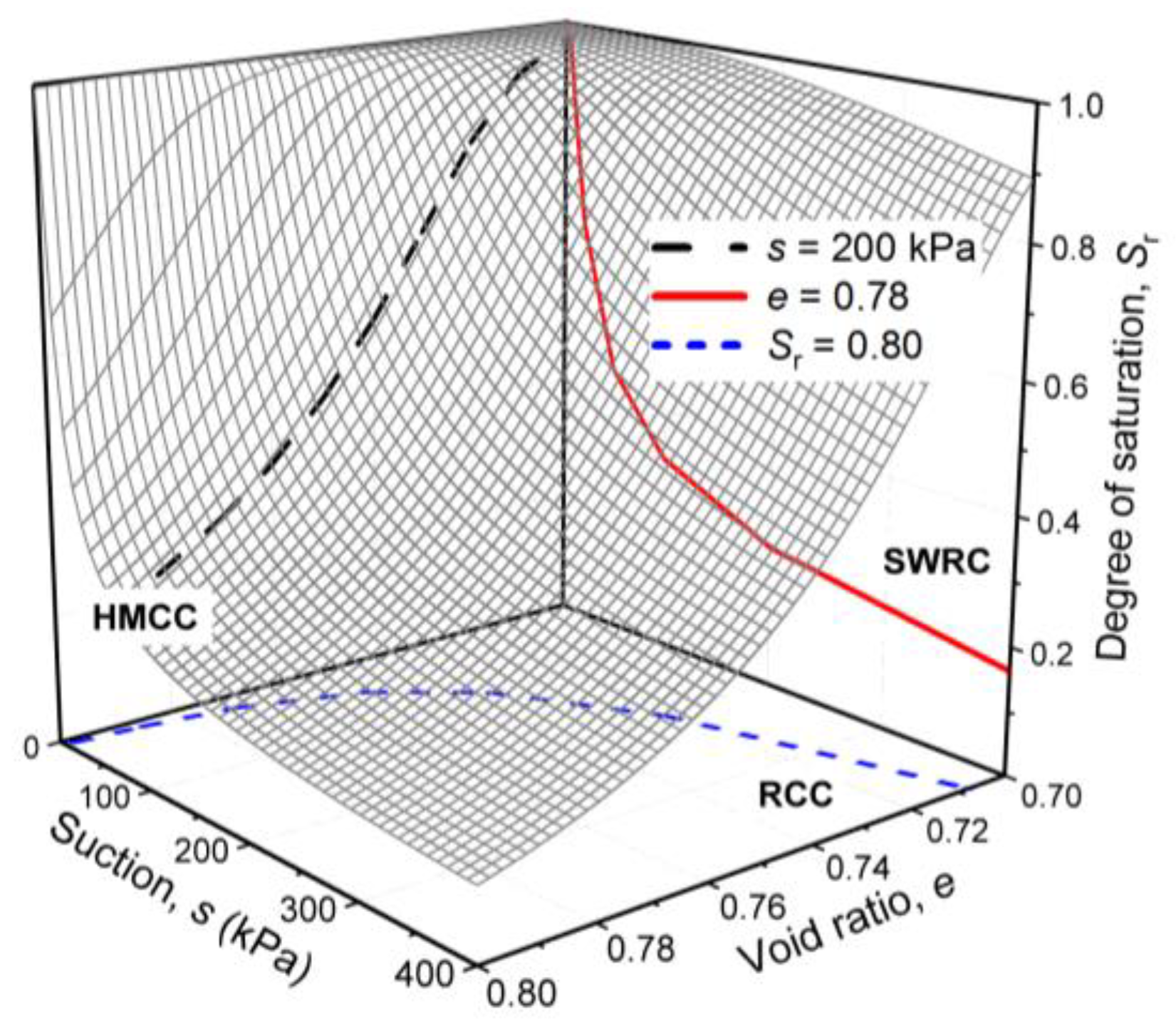
The advantages of using the SWRS and its projections in the rational interpretation of unsaturated soils’ behavior have been discussed in several studies [30,34,35]. However, detailed discussions on the projection characteristics of the SWRS on three planes (e, s, and Sr) remain outstanding in the current literature, irrespective of their significant importance. The SWRS has three different projection scenarios: projection at constant void ratio, e, and projection at constant suction, s and projection at constant degree of saturation, Sr. On the constant e plane, projections are a series of s–Sr relationships (i.e., SWRC). On the constant s plane, projections are a series of e–Sr relationships which reflect the changes in Sr due to the mechanical stress induced variation in e. In other words, the e–Sr relationships can reflect the influence of mechanical behavior on hydraulic behavior. On the constant Sr plane, projections are a series of s–e relationships indicating the dependence of mechanical behavior on hydraulic behavior. The s–Sr and e–Sr relationships are measurable using pressure plate and unsaturated triaxial tests, while the s–e relationship cannot be directly obtained.
In this study, to investigate the projection characteristics of the SWRS on the constant e, constant s, and constant Sr planes, three independent 2-D equations are formulated based on the SWRS model proposed by Gallipoli et al. [26]. The specific characteristics of the projections are discussed in detail. Modifications and improvements are also introduced with respect to (i) capturing the asymptotes and distinguishing the different behaviors in the high and low suction ranges for the s–Sr and e–Sr relationships and (ii) describing the s–e relationships.
2. Projections of the SWRS
Based on the van Genuchten [16] model, Gallipoli et al. [26] suggested Equation (1) for the SWRS:
where ψ, ω, m, and n are model parameters.
An example of the SWRS is shown in Figure 1 in the form of a surface mesh (its ψ, ω, n, and m values are 34.87, 0.002, 2.56, and 0.19) along with three specific projection curves obtained at s = 200 kPa, e = 0.78, and Sr = 0.80, respectively.
Three projection planes of the SWRS are succinctly described for providing background of how they can be used to describe the hydro-mechanical behavior of unsaturated soils:
- (i)
- The SWRCs: the Sr versus s plot at constant e (referred to as plane e).
- (ii)
- The Sr versus e plot where s is constant (referred as plane s). It is denoted as the hydro-mechanical coupling curves (HMCCs) in this paper.
- (iii)
- The s versus e plot at constant Sr (referred to as plane Sr). It is commonly referred to as the retention consolidation curves (RCCs).
The three projection planes were investigated using experimental data from the literature. Gallipoli [33] rewrote Equation (1) to Equation (2) in a logarithmic format.
Based on Equation (2), some interesting observations are derived from Gallipoli [33]:
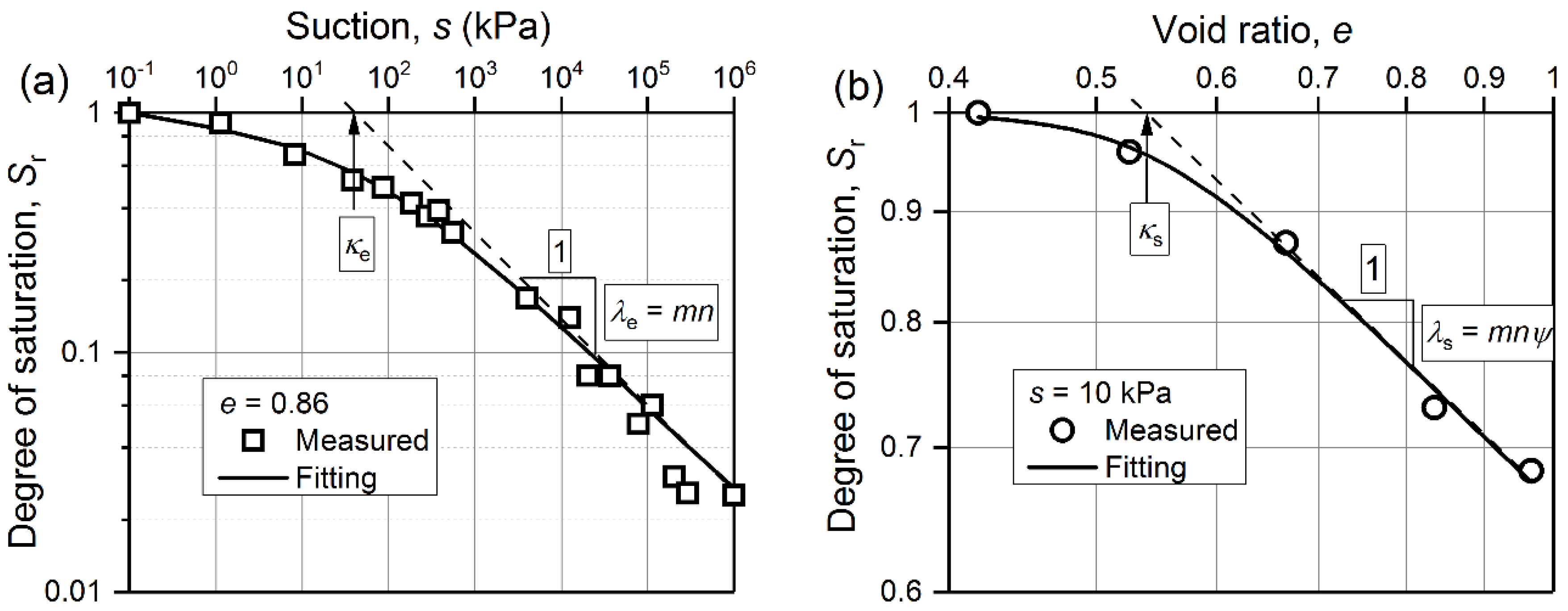
(i) For the main drying path, Equation (2) on the plane e (i.e., Sr versus s plot; SWRC) has an increasing negative tangent with decreasing Sr (defined in Equation (3) and shown in Figure 2a using data from Salager et al. [36]), and the tangent is equal to −mn (note that mn > 0) as Sr tends to zero. Similarly, Equation (2) on the plane s (i.e., Sr versus e plot; HMCC) has an increasing positive tangent with decreasing Sr and the tangent is equal to −mnψ (note that mnψ > 0) as Sr tends to zero (defined in Equation (4) and Figure 2b);
(ii) Equations (3) and (4) indicate that Equation (2) tends towards a planar asymptote in the logs–loge–logSr space when s and e tend to infinity and Sr tends to zero. Asymptotes expression of Equation (2) was defined as Equation (5);
(iii) when Equation (1) is rewritten in Equation (6) (where water ratio ew = eSr) and the product mnψ = 1, the log-planar asymptote (i.e., Equation (7)) is independent of void ratio.
Experimental data from eight soils from the published literature are used to examine the characteristics of the projections of SWRS on a logarithmic scale. Basic physical mechanical indices of these soils are summarized in Table 1.
3. Characteristics of the Projections of the SWRS
3.1. Soil-Water Retention Curves (SWRCs)
Equation (1) can be rewritten representing the plane e as below:
where e0 = initial void ratio at saturation; ψe, ωe, me, and ne are model parameters for plane e. Equation (8) converges to the van Genuchten [16] expression:
where α = ωe/(e0)ψe, indicating the air-entry suction; ne is a parameter related to pore-size distribution; me is a parameter related to the overall symmetry of the SWRC.
Equation (5) can be rewritten as:
From Equation (10), it can be observed that (i) when logs is approaching zero; logSr tends to mene logα, and (ii) when logSr tends to zero; logs tends to logα
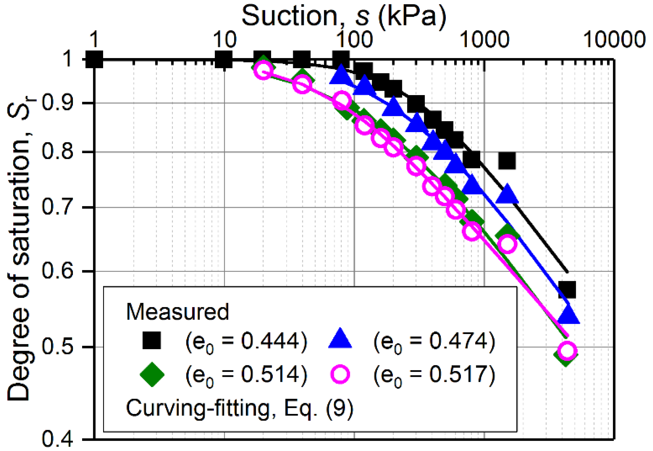
SWRCs of four soils summarized in Table 1 (i.e., the silty sand, compacted till, Ca-Bentonite, and Barcelona silt) are fitted using Equation (9). Figure 3 shows an example of the SWRCs of the compacted till measured by Vanapalli et al. [37] that move towards the left-hand side along the s axis with an increasing e0.
In Table 2, the values of parameters logα, me, ne in Equation (9) and λe (slope of asymptotes, see Figure 2a) and κe (horizontal intercept of asymptotes, see Figure 2a) for the four soils at different initial void ratios are summarized. The product mene is close to the absolute value of λe and the value of κe is close to logα. These two observations are consistent with the assumptions proposed by Gallipoli [33]. Therefore, relationships mene ≅ −λe and κe = logα are applied in the later sections to determine the position of asymptotes.
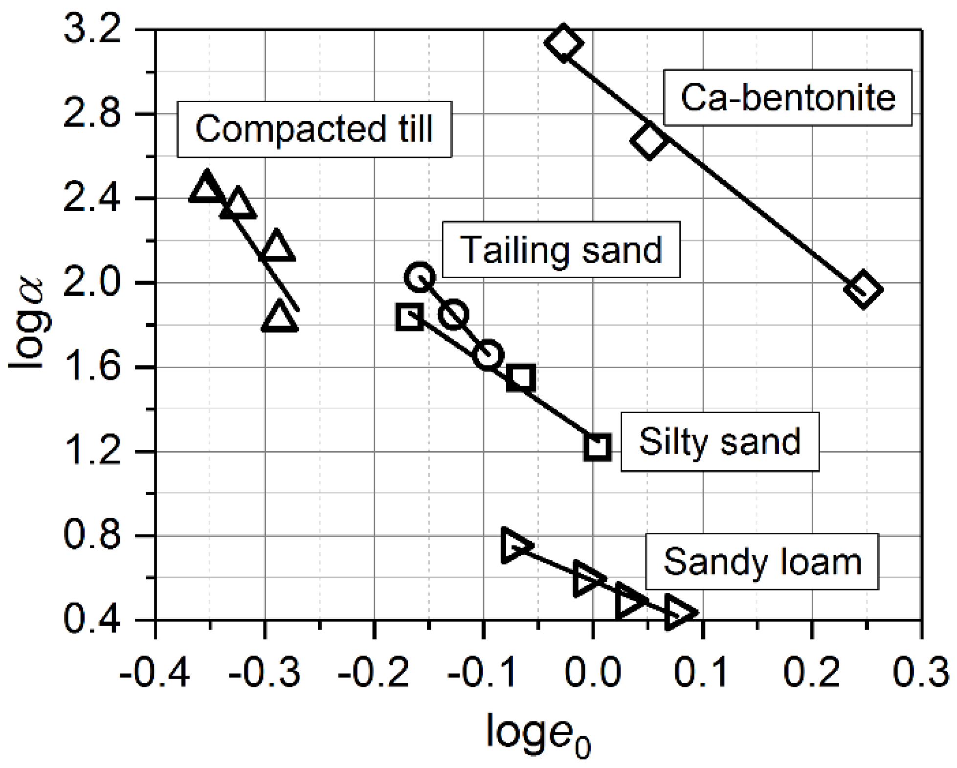
By taking log on both sides of the equation, α = ωe/(e0)ψe yields logα = logωe − ψe loge0. The ψe is the slope of the logα–loge0 relationship and logωe is the vertical intercept of the logα–loge0 line at loge0 = 0. Figure 4 shows the logα–loge0 relationships for the four soils. The results in Figure 4 are consistent with the conclusion of Stange and Horn [43], who found linear relationships between loge0 and logα.
Gallipoli [33] suggested that SWRCs at different initial void ratios can be obtained through a rigid translation from a reference SWRC along the s axis in the logs–logSr plane. Similarly, HMCC at different suction can be obtained by a rigid translation from a reference HMCC along the e axis in the loge–logSr plane. A rigid translation implies that all asymptotes of the SWRCs at different initial void ratios are parallel to each other and their mene values are identical. In other words, the horizon distance between two asymptotes at different initial void ratios is constant and equals to the horizon distance between the intercepts of the two asymptotes at logs = 0. This is consistent with the postulation proposed by Nuth and Laloui [28] that the SWRC has an intrinsic shape at constant e0 and this intrinsic curve were parallel to the SWRCs at all constant values of e0.
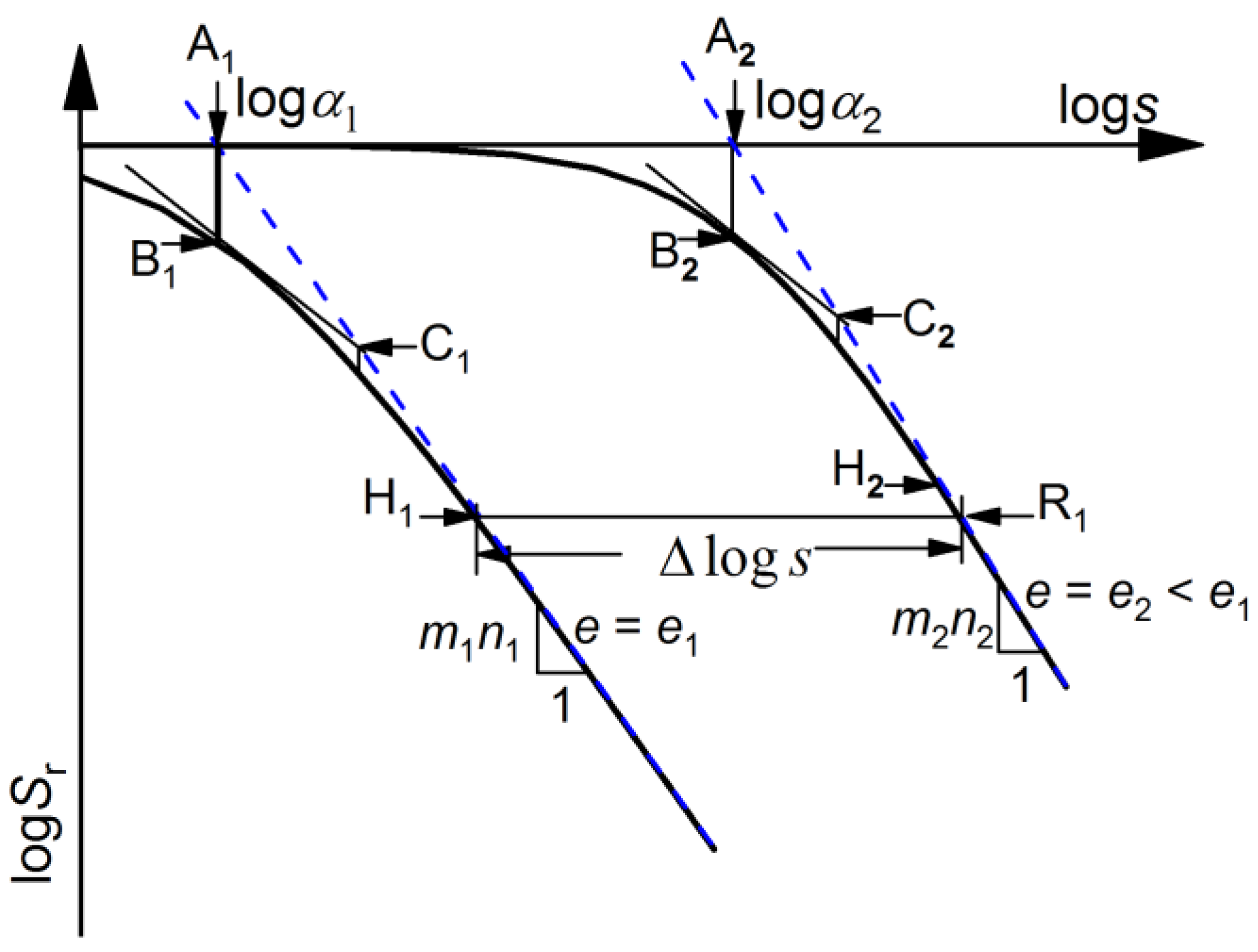
In order to quantitatively capture the asymptotes, an approximate approach shown in Figure 5 is proposed. For two SWRCs with different initial void ratio e1 and e2 (e2 < e1), α1, m1, n1 and α2, m2, n2 are their parameter values of Equation (9), and λ1, κ1 and λ2, κ2 are the respective slope and horizontal intercept of asymptotes. Two coordinate points are required for determining the asymptotes: one point is A1 (logα1, 0) or A2 (logα2, 0) which are easily obtained; the other point can be indirectly obtained from the SWRC, referred to as matching point. According to m1n1 ≅ −λ1 and m2n2 ≅ −λ2, the matching point must satisfy the condition that the absolute value of the slope calculated by the two points (i.e., point A and the matching point) is close to the value of the product m1n1 (or m2n2). In order to obtain the matching point, an iteration-based tangential approximation method can be used, which is detailed below.
Point B1 is the vertical projection of point A1 on the corresponding SWRC (see Figure 5). Substituting the abscissa value of point A1 into Equation (2), point B1 can be obtained, namely (logα1, m1log(1/2)). A tangent line of the SWRC at point B1 can be conveniently defined using the slope of the SWRC defined in Equation (3) and point B1 (i.e., logSr = −1/2⋅m1n1⋅(logs − logα1) + m1log(1/2)). With this tangent line and the asymptote of the SWRC passing point A1 (defined by Equation (10)), point C1 can be obtained at the intersection (see Fig 5) and its coordination is (logα1 − 1/n1·log(1/4), m1log(1/4)). The first iteration (A1→B1→C1) ends here. Taking point C1 as the starting point (similar to A1), one can continue with the next iteration using the same approach detailed for first iteration. This procedure is repeated until a matching point is found. The matching point is the point where the starting point overlaps with its projection on the SWRC, and typically can be determined within seven iterations. The matching point obtained after seven iterations is denoted as point H1 (logα1 + 1.5382/n1, −1.5506m1). The slope calculated by both points A1 and H1 is about equal to −1.008m1n1, meeting the necessary condition of m1n1 ≅ −λ1. Therefore, the asymptotes can be well captured by points A1 and H1. The proposed procedure is an objective and simple procedure to determine the asymptote. It is assumed that any points on the SWRC after point H1 belong to the asymptote.
A simplified calibration process proposed by Gallipoli [33] was used to further validate whether the asymptote determined by points A1 and H1 is reasonable. The purpose of the proposed calibration is to ensure that the value of the product m1n1 estimated from linear best-fitting of experimental data (Equation (10)) is consistent with a logarithmic planar behavior over the experimental data range. Gallipoli [33] suggested that the values of m1 and n1 are considered acceptable if logSr < −m1 over the experimental asymptotic range (m1 and n1 are obtained from the product m1n1 value using the relationship m1 = 1 − 1/n1 proposed by van Genuchten [16]); otherwise, they have to be recalibrated by imposing logSr,max = −m1, where Sr,max is the maximum experimental value of the degree of saturation. Considering that logSr = −1.5506m1 < −m1 for the matching point H1(logα1 + 1.5382/n1, −1.5506m1), the asymptote computed by points A1 and H1 using the proposed method satisfies the criterion logSr < −m1 suggested by Gallipoli [33] and captures the logarithmic planar behavior over the experimental range.
In order to investigate the relationship between asymptotes of two main drying curves at different values of e1 and e2, the horizontal projection of point H1 on the SWRC at e2 can be obtained and is denoted as R1 (logα2 + 1.5506m1/m2n2, −1.5506m1). The horizontal distance between point H1 and point R1 in log-log scale is (see Figure 5):
Δlogs ≅ log (α2/α1) when m1n1 is close to m2n2. In this case, asymptotes of two main drying curves at different values of e1 and e2 are parallel. It can be seen from Table 2 that the product mene of the same soil are almost the same at different values of the initial void ratio for some soils (such as silt sand, compacted till and Ca-bentonite). Therefore, their main drying curves are parallel.
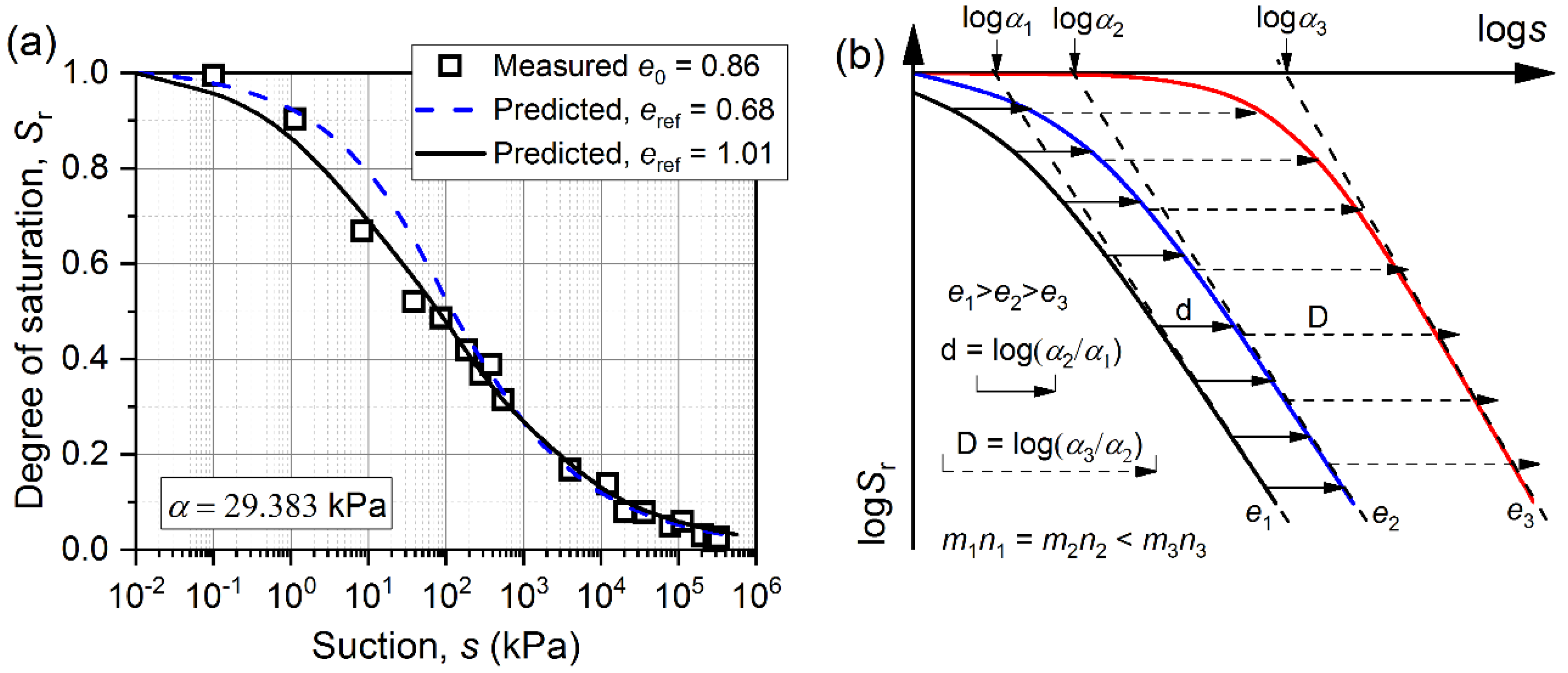
The SWRCs however may not be parallel but controlled by both mene and αe, if mene values are not close. An example is shown to highlight this scenario using data of a silty sand (soil properties are summarized in Table 1 and mene and αe values are summarized in Table 2). Assume its two SWRCs at e0 = 0.68 and 1.01 are available and used as reference curves, while the SWRC at e0 = 0.86 is used to provide comparisons between the predictions and measurements. Considering the linear relationships between loge0 and logα, the α value of the SWRC at e0 = 0.86 can be obtained from the linear relationship defined by loge0 and logα of the reference SWRCs at e0 = 0.68 and 1.01. As shown in Figure 6a, for SWRCs at e0 = 0.86, the predicted curve (solid line) obtained by a rigid translation of the reference SWRC at e0 = 1.01 shows better agreements with measurements than the predicted curve translated from the reference SWRC at e0 = 0.68 (dash line). It can be seen from the summarized information in Table 2 that the deviation from logα values of the SWRCs at e0 = 0.86 to the logα values of the reference SWRCs at e0 = 1.01 and e0 = 0.68 are 0.251 and 0.367, respectively. This means that the smaller deviation of logα is, the higher the accuracy of the prediction is. In addition, mene values of reference SWRC at e0 = 1.01 are also closer to the mene values of SWRC at e0 = 0.86, which contributes to a better prediction.
In addition, Figure 6b shows three hypothetic SWRCs at e1, e2, and e3, respectively, for further explanation. mn values of SWRCs at e1 and e2 are close but different from that of SWRCs at e3. When mn values of two SWRCs (e.g., SWRCs at e1 and at e2) are close, their horizon distance d is mainly controlled by their logα values. On the contrary, when mn values of two SWRCs (e.g., SWRCs at e2 and at e3) are different, their horizon distance D is controlled by both mn and logα. This is also reflected in Equation (11). The equal-length arrows in Figure 6b indicates the horizontal distance between two SWRCs can be determined by their logα only (arrows with solid lines indicate shifting from SWRC at e1 to SWRC at e2 and arrows with dash lines indicate shifting from SWRC at e2 to SWRC at e3). As can be seen from Figure 6b, the horizontal shifting works well for SWRCs at e1 and at e2 as the arrows reach the SWRC at e2. On the contrary, such horizontal shifting introduces errors for SWRCs at e2 and at e3 as the arrows do not always stop at the SWRC at e3.
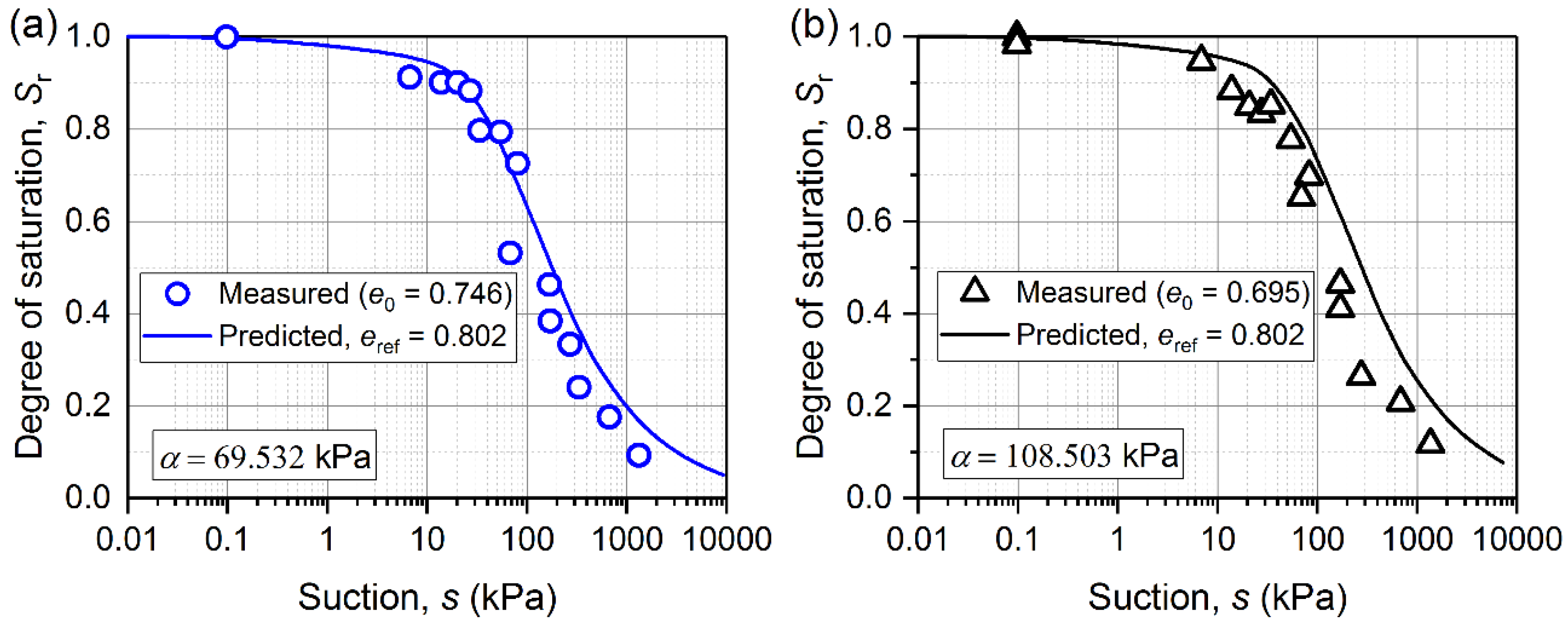
The products mene in Table 2 are not always identical for different values of initial void ratios for some soils (such as tailing sand and sandy loam). To further validate the curve shifting method, Figure 7 shows predicted SWRCs obtained by a rigid translation of the same reference SWRC (e0 = 0.802) for a tailing sand. Some differences in predictions and the measurements can be observed from the summarized information in Figure 7. These differences may be attributed to the two factors; (1) the difference in mn values, and (2) the difference in logα or e0 values. For the former, deviations in the mn values of the predicted SWRCs (at e0 = 0.746 and e0 = 0.695) and the reference SWRC (at e0 = 0.802) are about 0.13 and 0.30 (see Table 2). Similarly, for the latter, deviations in the e values of the predicted SWRCs (at e0 = 0.746 and e0 = 0.695) and the reference SWRC (at e0 = 0.802) are 0.056 and 0.107. Predictions using SWRC at e0 = 0.746 as reference curve is slightly better than that using SWRC at e0 = 0.695 as a reference curve due to the smaller deviation in the mn and e0 values.
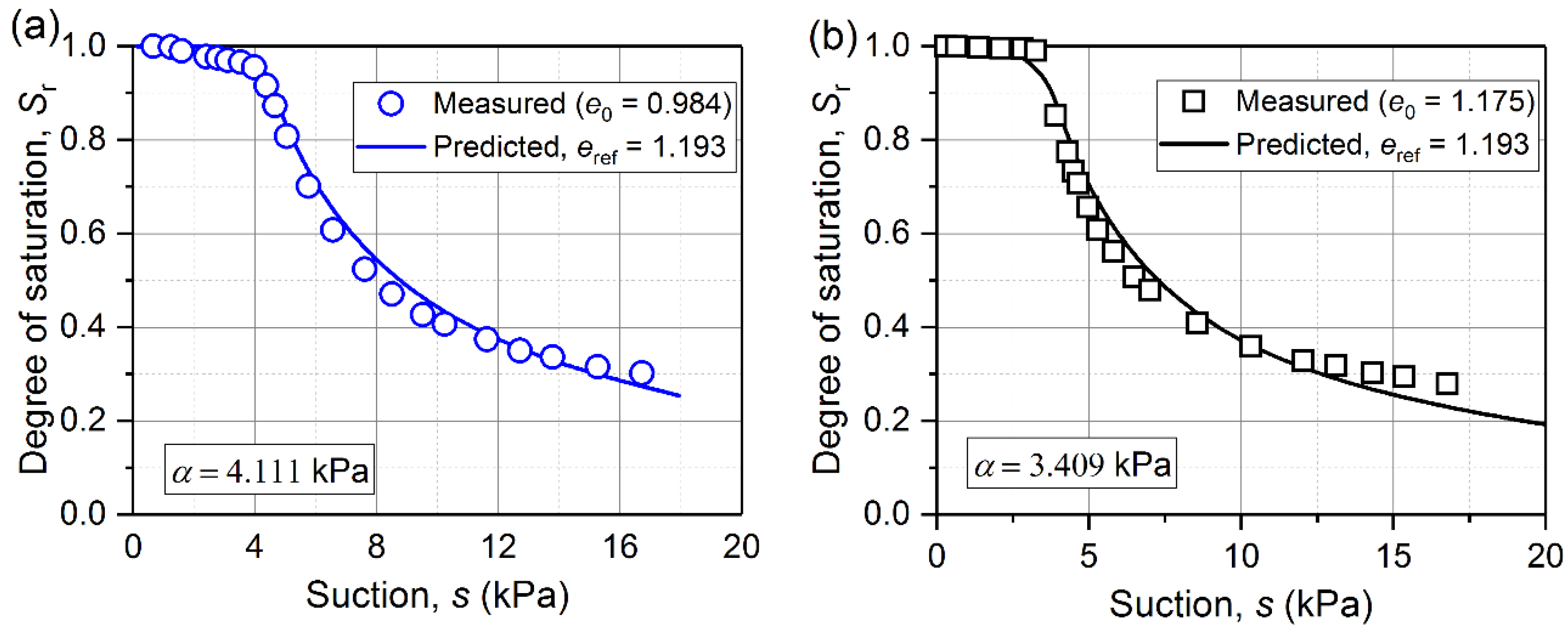
Another example for the sandy loam in Table 2 is shown in Figure 8. When the deviations in mn and e0 are small, predicted SWRCs (e0 = 0.984 and 1.175) obtained by a rigid translation of the same reference SWRC (eref = 1.193) show a good agreement with the experimental data. Therefore, three aspects deserve attention when predicting SWRCs at constant e0 using the curve shifting method: (1) at least two sets of SWRCs with different initial void ratios experimental data must be known to estimate the parameter α values of Equation (9) and the linear relationships between loge0 and logα; (2) the reference curve has to be fitted by Equation (9) prior to translation because of typical limitations of the experimental data; (3) the difference between the e0 values of the predicted SWRCs and reference SWRCs should be as small as possible.
3.2. Hydro-Mechanical Coupling Curves (HMCCs)
Equation (1) is rewritten for interpreting HMCCs in the following way:
where scon = constant suction; ψs, ωs, ms, and ns are model parameters for the constant suction condition.
Equation (5) can be rewritten as:
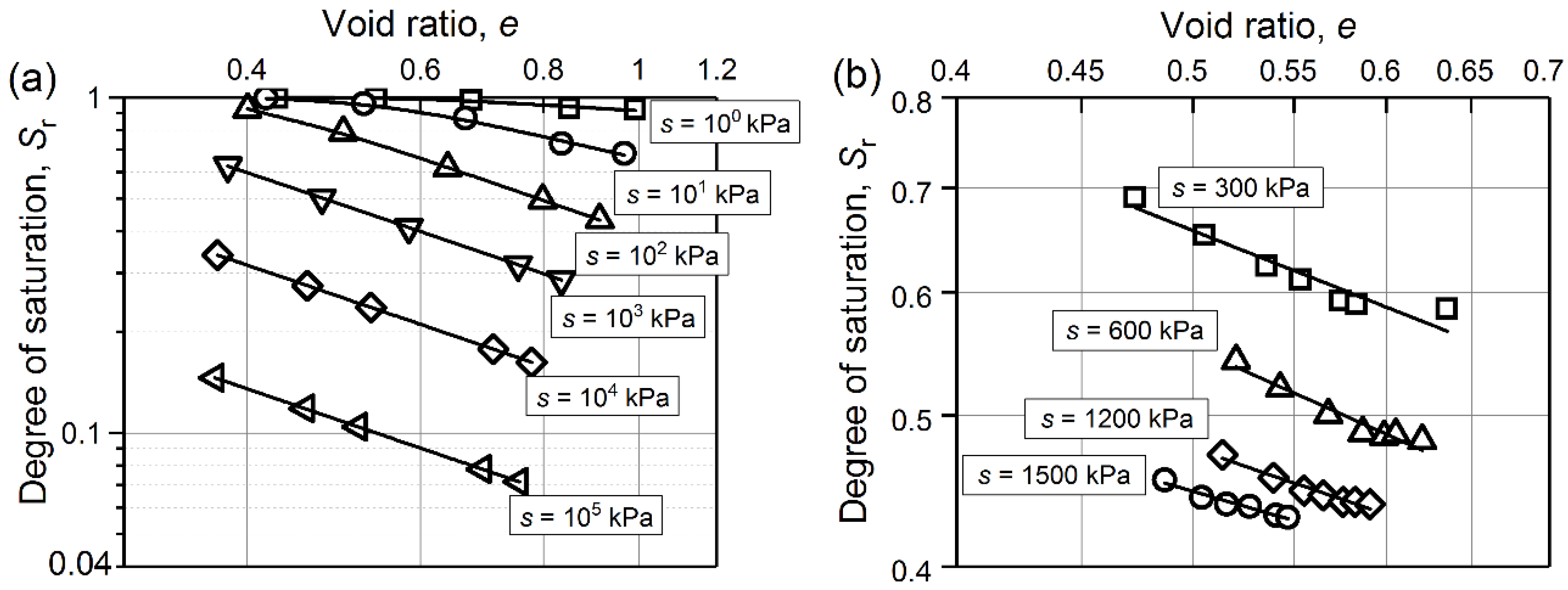
where logβ = log(ωs/scon)/ψs. Equation (13) is the asymptote of Equation (2) on the plane s. When loge tends to zero, logSr tends to msnsψs·logβ. Meanwhile, loge tends to logβ when logSr tends to zero. Figure 9 shows the evolution of experimental HMCCs in loge–logSr plane at different constant s using data obtained from Salager et al. [36] and Sun and Sun [42]. The results indicate that HMCCs move to the left-hand side along the e axis with increasing suction.
The HMCCs parameters β, ms, ns and λs, κs for four soils used in this study at different constant suctions are summarized in Table 3. The λs is the slope of asymptotes and κs is horizontal intercept of asymptotes (see Figure 2b). It can be observed from Table 3 that: (i) the product msnsψs is close to the absolute value of λs, namely msnsψs ≅ −λs and (ii) κs is approximately equal to logβ, namely logβ ≅ κs. Note that CDG and CDE in Table 3 denote different stress paths for the constant suction, respectively. Unlike the logs–logα relationships shown in Figure 4 which are linear, the logscon–logβ relationships are bi-linear.
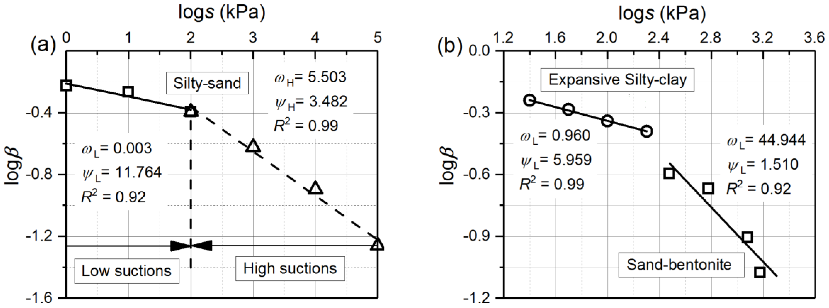
Figure 10 highlights such a relationship for silty-sand, expansive silty-clay, and a sand–bentonite mixture. These results suggest the relationship logβ = log(ωs/scon)/ψs is less effective in fitting the data over the entire suction range. Due to this reason, Equation (14) is proposed to separately describe the logscon-ogβ relationships in the low and high suction ranges.
Subscripts L and H denote low suction and high suction; ψL, ψH, ωL, ωH, βL, βH are parameters. In addition, ψL and ωL (or ψH and ωH) have a clear physical meaning as they are associated with the slope and intercept of the straight line interpolating experimental data in the logscon–logβ plane at low or high suctions.
To use Equation (14), it is important to distinguish low and high suction ranges. Interestingly, the asymptote (i.e., Equation (7)) is independent of the e when the product mnψ = 1 in the loge-logs-logew space [33]. Tarantino [32] presented a model similar to the Gallipoli [26] expression. This model satisfies the condition of mnψ = 1, and the precondition for this model is that the suction has to be located in the high suction range. Therefore, constant suctions imposed on the HMCC can be considered as high suctions when the product msnsψs = 1. It is important to note that the product msnsψs is not always equal to 1 (see Table 3, for instance the case for the sand-bentonite and expansive silty-clay). For this reason, the imposed constant suctions will be regarded as low suctions when 0 < mnψ < 1. Combining with this conclusion and several sets of data related to silty sand (i.e., scon and logβ) in Table 3, a bilinear relationship exists in the logscon–logβ plane over the full suction range (see Figure 10a). It is evident for the tested silty sand that 100 kPa can be considered as the critical suction value for distinguishing low suctions from high suctions. This conclusion is consistent with the results of Salager et al. [34,36] obtained from a graphical approach that above 100 kPa suction, SWRCs with different initial void ratios can be regarded as an overlapping curve on the constant e plane. Figure 10b shows that there is a well-defined linear relationship between logscon and logβ at low suctions for sand-bentonite and expansive silty clay.
For some soils, it is likely that the value of msnsψs departs significantly from the absolute value of λs. A novel method is suggested in the present study to assure msnsψs ≅ −λs:
(i) When msnsψs > 1 and not equal to −λs, msnsψs is assumed equal to 1 and relationship ms = 1/(nsψs) is substituted into Equation (12) to fit the experimental data. This results in a new set of ms, ns, and ψs values. If the new product msnsψs is close to −λs, then the ms, ns, and ψs values are deemed suitable. If still msnsψs significantly departs from −λs, additional calibration is needed. In this case, the new ms, ns, and ψs values are used to plot the HMCC and the λs of the plotted HMCC is determined (this updated λs is denoted as λs*). Substitute relationship ms = λs*/(nsψs) into Equation (12) again to update ms, ns, and ψs values until msnsψs ≅ −λs is achieved. The final ms, ns, and ψs values satisfying msnsψs ≅ −λs are deemed acceptable.
(ii) When 0 < msnsψs < 1 and msnsψs ≠ −λs, as a first step it is assumed equal to −λs and then substituted into Equation (12). The subsequent processing is the same as for the msnsψs > 1 case, which was detailed in the earlier step (i).
The advantage of this method is that both low suctions and high suctions can be clearly distinguished by the values of the product msnsψs. The product msnsψs is approximately equal to −λs after three iterations for the data of Table 3 (bold fonts). In addition, Equation (12) with new parameter values provides a good match with experimental data. Hence, the calibration method proposed in this paper is reasonable.
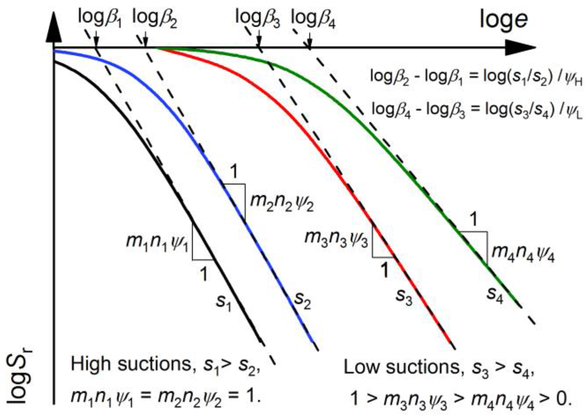
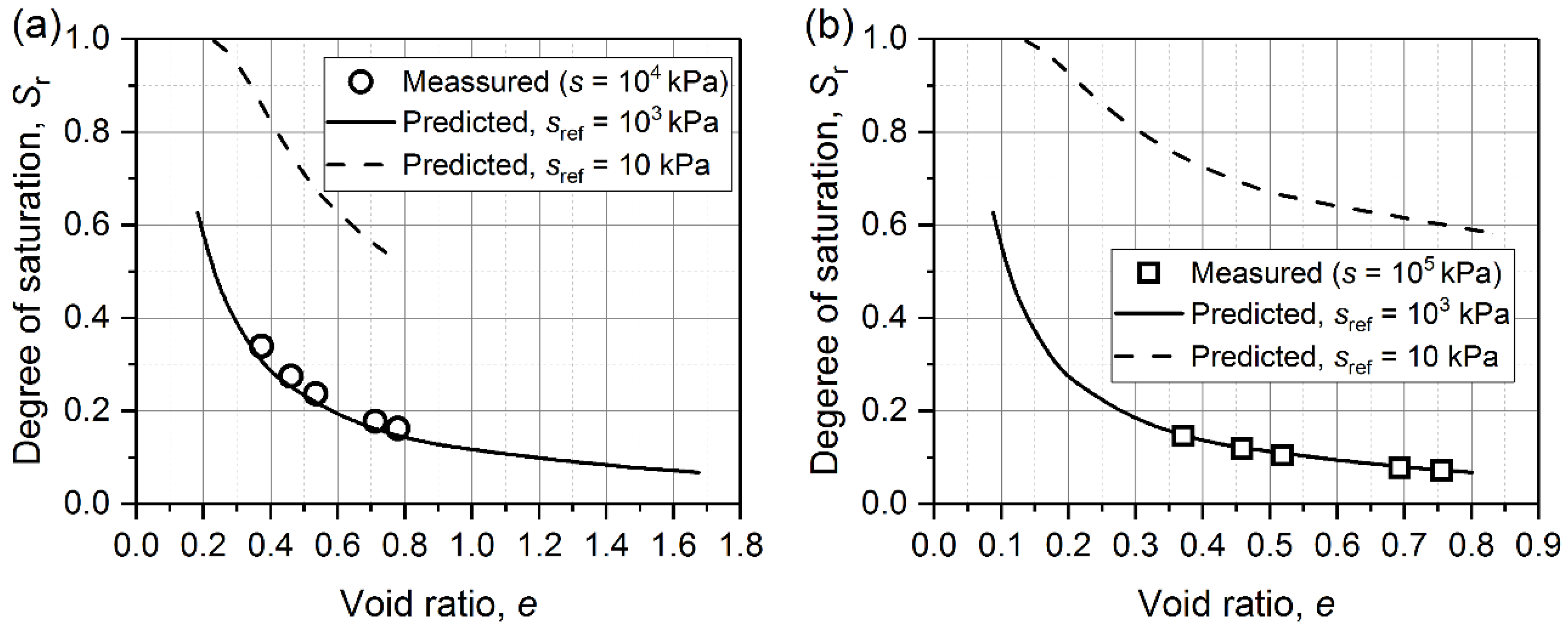
Figure 11 shows a schematic diagram of the HMCCs with different constant suction values at low suctions and high suctions. Among them, miniψi and logβi are the parameter values of Equation (13) corresponding to different constant suctions si (i = 1, 2, 3, 4). Dash lines stand for asymptotes of HMCCs (solid lines) on a logarithmic scale. All HMCCs at high suctions (i.e., msnsψs = 1) can be obtained by a rigid translation of the same graph in the loge–logSr plane [33]. On the contrary, the values of the product msnsψs at low suctions (0 < msnsψs < 1) are different. Due to this reason, HMCCs at high suctions may not be obtained by extending this rigid translation technique from a reference HMCC at low suctions. In other words, rigid translation is only feasible in high suction range or in low suction range, separately. Rigid translation from high suction range to low suction range or vice versa is not reliable. Figure 12 shows predicted HMCCs (at s = 104 kPa and 105 kPa) obtained by a rigid translation of two reference HMCCs (sref = 103 kPa and 10 kPa) for a silty sand. The translation between the prediction HMCC and the reference HMCC is evaluated by term: |logβref − logβpre| = |log(spre/sref)/ψ|. The values of ψ can be obtained by Equation (14) and (15), where logβi and si are given in Table 3 (ψL = 0.085 and ψH = 0.320). It is evident that using the reference HMCC at low suctions to predict HMCCs at high suctions can lead to deviations that are significant from the experimental data.
The method of tangential approximation described in the SWRCs section was followed to investigate the relationship between asymptotes of two main drying curves at different values of s1 and s2. For a given pair of low suction values of s1′ and s2′ (s2′ < s1′), the constant horizontal distance between the two asymptotes is presented in Equation (16):
where ω1′, ψ1′, m1′, n1′ and ω2′, ψ2′, m2′, n2′ are two sets of parameter values of Equation (12) corresponding to HMCCs at s1 and s2, respectively. β1′= (ω1′/s1)1/ψ1’ and β2′ = (ω2′/s2)1/ψ2’. Δloge can be considered approximately equal to log(β2′/β1′) when m1′n1′ψ1′ is close to m2′n2′ψ2′. To simplify and facilitate the application, it is convenient to assume that ω1′ = ω2′ = ωL and ψ1′ = ψ2′ = ψL for low suction ranges, the horizontal distance between the predicted HMCC and the reference HMCC is Δloge = log(s1/s2)/ψL. A trial calculation method is introduced to improve prediction accuracy of the parameter ψs, in addition to Equation (14) which can be directly used to determine ψs.
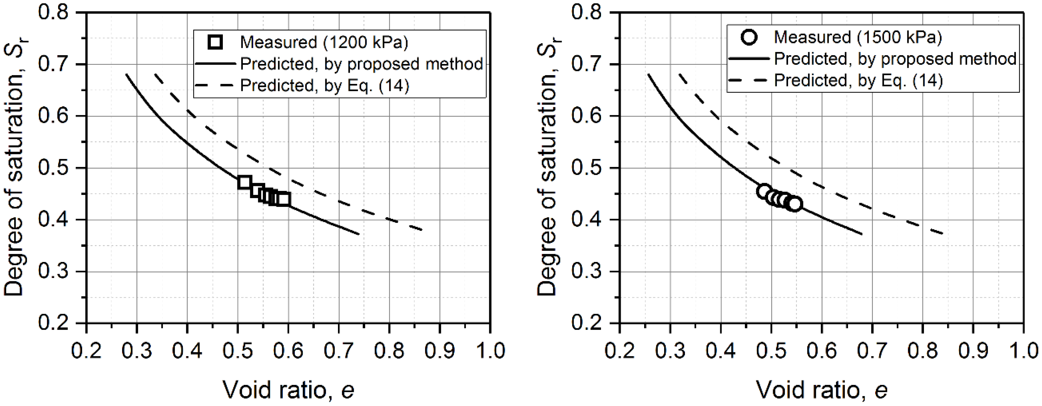
The trial calculation method is explained using two sets of HMCC data for a sand bentonite that are summarized in Table 3. The data of HMCCs at s = 300 kPa and 600 kPa are taken as reference curves. The horizontal distance between these two reference HMCCs is Δloge = log(600/300)/ψL. Different ψL values can be tried to obtain the Δloge and therefore translate the HMCC at s = 300 kPa to HMCC at s = 600 kPa. A suitable ψL value is obtained when the translated HMCC at s = 600 kPa fits the measurements of the HMCC at s = 600 kPa. The HMCCs with different constant suctions obtained by a rigid translation of the reference HMCC (s = 300 kPa) and compared with experimental data (see Figure 13) to check validity of the proposed method. The results show predicted HMCCs obtained from the proposed method match well with experimental data. Therefore, the curve shifting method proposed by Gallipoli [33] is also feasible at low suctions.
Similarly, three aspects also need to be considered when predicting HMCCs at constant s using the curve shifting method: (1) at least two sets of HMCCs with different constant suctions test data must be known to estimate the ψ, and the trail calculation method proposed in this section to refine the ψ can be considered; (2) The reference curve needs to be fitted by Equation (12) prior to translation; (3) HMCCs in high suction range may be obtained from a rigid translation of a reference HMCC high suction range and rigid translation can also be used in the same way in the low suction range. However, HMCCs at high suctions cannot be obtained from a rigid translation of a reference HMCC at low suctions.
3.3. Retention Consolidation Curves (RCCs)
Equation (1) is rewritten into Equation (17) for interpreting the RCC.
where Srcon = constant degree of saturation; ψsa, ωsa, msa, and nsa are model parameters. The derivation of RCCs in the logs–loge plane at Srcon is obtained as
It is difficult to measure s–e curves at constant Sr (i.e., RCC) from experimental studies. In order to represent the RCC, the SWRS (i.e., Equation (1)) shall be determined from measurements of the SWRCs at different void ratios or HMCCs at different suctions first and then set Sr to constant to obtain the RCC. Salager et al. [36] measured SWRCs of a clayey silt sand. The five sets of experimental data are fitted by Equation (1) with best-fit parameter values ψ = 4.180, ω = 11.335, n = 0.686, and m = 0.565. RCCs at different constant Sr are obtained by substituting these parameter values into Equation (17). As shown in Figure 14, RCCs are linear in the logs–loge plane, and their slope equals to −1/ψsa. The RCCs move towards the left-hand direction along the s axis with the increase in constant Sr.
It should be noted that void ratio calculated from Equation (17) may exceed 1 at low suction levels, which is erroneous (see Figure 14a). On the other hand, specimens after compaction are typically unsaturated and have different initial suction levels. RCCs in Figure 14a should start from the initial suction and degree of saturation after compaction rather than from saturated condition (which is Sr = 1 and s = 0.1 kPa in Figure 14a).
Salager et al. [34] presented a relationship (Equation (19)) between the void ratio and suction using five sets of experimental data.
where a1, b1, c1, d1, and χ are empirical parameters. The values of a1, b1, c1, d1, and χ are 1000, 400, 0.466, 2.896, and 0.21, respectively, which was suggested by Salager et al. [34].
For a saturated specimen with e0, its initial suctions and corresponding void ratios at different constant Sr can be obtained from the simultaneous solution of Equation (17) and Equation (19). As a result, these initial suctions and corresponding void ratios would form a curve, which is called the modified curve in this study. As shown in Figure 14b, the short-dashed line is a modified curve that shows initial states of unsaturated soil specimens at different constant Sr. The modified curve shows that the initial suction is increasing with the reducing constant Sr. For different e0 (i.e., 0.44, 0.68, and 1.01) in Figure 14b, the initial suction is decreasing as e0 increases at equal Sr. Such a behavior is expected because at equal Sr, the water content is increasing as initial void ratio increases based on Sr = Gsw/e0, resulting in the decrease of suction. Hence, modified curves proposed in this study are reasonable.
4. Conclusions
Based on the SWRS model of Gallipoli et al. [26], three independent 2-D equations were presented in this paper and used to investigate the projection characteristics of the SWRS on the constant e, s, and Sr planes in order to have an insight into the hydromechanical behavior of unsaturated soils. The details are summarized below:
- (1)
- The SWRCs tend to move towards the left-hand direction along the s axis on a log-log scale with the increase in initial e. When the gap of initial e values between the predicted SWRCs and reference SWRCs is as small as possible, SWRCs at different initial e can be obtained by a rigid translation of a reference SWRC alone the s axis in the logs-logSr plane.
- (2)
- Similarly, the HMCCs and the RCCs move towards the left-hand direction along the e axis on a log-log scale with the increase in s and Sr, respectively. HMCCs at high suctions cannot be obtained from a rigid translation of a reference HMCC at low suctions. The constant suctions imposed on the HMCCs are suggested to be high suctions when the mnψ = 1 and low suctions when 0 < mnψ < 1 (i.e., m, n, and ψ are the Gallipoli et al. [26] model parameters).
- (3)
- The RCC equation proposed is capable of describing the relationship between e and s on the constant Sr plane. The modified RCCs show that the initial suction increases with the reducing constant Sr. Moreover, the initial suction is reducing as initial e increases at equal values of Sr.
Author Contributions
Conceptualization, W.Z.; writing—original draft preparation, Y.Y.; writing—review and editing, W.Z. and Z.H.; supervision, W.Z. and Z.H.; funding acquisition, W.Z. and Z.H.
Funding
This research was funded by the National Natural Science Fund of China (No. 51479148 and 51809199).
Conflicts of Interest
The authors declare no conflict interest.
References
- Alonso, E.E.; Gens, A.; Josa, A. A constitutive model for partially saturated soils. Geotechnique 1990, 40, 405–430. [Google Scholar] [CrossRef] [Green Version]
- Vaunat, J.; Romero, E.; Jommi, C. An elastoplastic hydromechanical model for unsaturated soils. In International Workshop on Unsaturated Soils: Experimental Evidence and Theoretical Approaches in Unsaturated Soils; Tarantino, A., Mancuso, C., Eds.; Springer: Balkema, Rotterdam, 2000; pp. 121–138. [Google Scholar]
- Wheeler, S.; Sharma, R.; Buisson, M. Coupling of hydraulic hysteresis and stress-strain behavior in unsaturated soils. Geotechnique 2003, 53, 41–53. [Google Scholar] [CrossRef]
- Khalili, N.; Habte, M.; Zargarbash, S. A fully coupled flow deformation model for cyclic analysis of unsaturated soils including hydraulic and mechanical hystereses. Comput. Geotech. 2008, 35, 872–889. [Google Scholar] [CrossRef]
- Gens, A. Soil–environment interactions in geotechnical engineering. Geotechnique 2010, 60, 3–74. [Google Scholar] [CrossRef]
- Sheng, D.C.; Zhou, A.N. Coupling hydraulic with mechanical models for unsaturated soils. Can. Geotech. J. 2011, 48, 826–840. [Google Scholar] [CrossRef]
- Sun, D.A.; Cui, H.B.; Matsuoka, H.; Sheng, D.C. A three-dimensional elastoplastic model for unsaturated compacted soils with hydraulic hysteresis. Soils Found. 2007, 47, 253–264. [Google Scholar] [CrossRef]
- Fuentes, W.; Triantafyllidis, T. Hydro-mechanical hypoplastic models for unsaturated soils under isotropic stress conditions. Comput. Geotech. 2013, 51, 72–82. [Google Scholar] [CrossRef]
- Masin, D. Double structure hydromechanical coupling formalism and a model for unsaturated expansive clays. Eng. Geol. 2013, 165, 73–88. [Google Scholar] [CrossRef]
- Gao, Y.; Sun, D.A.; Zhou, A.N. Hydro-mechanical behaviour of unsaturated soil with different specimen preparations. Can. Geotech. J. 2016, 53, 909–917. [Google Scholar] [CrossRef]
- Ghasemzadeh, H.; Sojoudi, M.H.; Amiri, S.A.G.; Karami, M.H. Elastoplastic model for hydro-mechanical behavior of unsaturated soils. Soils Found. 2017, 57, 371–383. [Google Scholar] [CrossRef] [Green Version]
- Wheeler, S.; Sivakumar, V. An elasto-plastic critical state framework for unsaturated soils. Géotechnique 1995, 45, 35–53. [Google Scholar] [CrossRef]
- Cui, Y.; Delage, P. Yielding and plastic behaviour of an unsaturated compacted silt. Geotechnique 1996, 46, 291–311. [Google Scholar] [CrossRef]
- Gardner, W.R. Some steady state solutions of the unsaturated moisture flow equation with application to evaporation from a water-table. Soil Sci. 1958, 85, 228–232. [Google Scholar] [CrossRef]
- Brooks, R.H.; Corey, A.T. Hydraulic Properties of Porous Media; Colorado State University: Fort Collins, CO, USA, 1964. [Google Scholar]
- Van Genuchten, M.T. A closed-form equation for predicting the hydraulic conductivity of unsaturated soil. Soil Sci. Soc. Am. J. 1980, 44, 892–898. [Google Scholar] [CrossRef]
- Fredlund, D.G.; Xing, A.Q. Equations for the soil-water characteristic curve. Can. Geotech. J. 1994, 31, 521–532. [Google Scholar] [CrossRef]
- Ng, C.W.W.; Pang, Y.W. Influence of stress state on soil-water characteristics and slope stability. J. Geotech. Geoenviron. 2000, 126, 157–166. [Google Scholar] [CrossRef]
- Assouline, S. Modeling the relationship between soil bulk density and the water retention curve. Vadose Zone J. 2006, 5, 554–562. [Google Scholar] [CrossRef]
- Sun, D.A.; Sheng, D.C.; Xu, Y.F. Collapse behaviour of unsaturated compacted soil with different initial densities. Can. Geotech. J. 2007, 44, 673–686. [Google Scholar] [CrossRef]
- Miller, G.A.; Khoury, C.N.; Muraleetharan, K.K.; Liu, C.; Kibbey, T.C.G. Effects of soil skeleton deformations on hysteretic soil water characteristic curves: Experiments and simulations. Water Resour. Res. 2008, 44. [Google Scholar] [CrossRef]
- Masin, D. Predicting the dependency of a degree of saturation on void ratio and suction using effective stress principle for unsaturated soils. Int. J. Numer. Anal. Methods Geomech. 2010, 34, 73–90. [Google Scholar] [CrossRef]
- Zhou, A.N.; Sheng, D.; Carter, J.P. Modelling the effect of initial density on soil-water characteristic curves. Geotechnique 2012, 62, 669–680. [Google Scholar] [CrossRef]
- Han, Z.; Vanapalli, S.K.; Zou, W.L. Integrated approaches for predicting soil-water characteristic curve and resilient modulus of compacted fine-grained subgrade soils. Can. Geotech. J. 2017, 54, 646–663. [Google Scholar] [CrossRef] [Green Version]
- Huang, S.; Barbour, S.L.; Fredlund, D.G. Development and verification of a coefficient of permeability function for a deformable unsaturated soil. Can. Geotech. J. 1998, 35, 411–425. [Google Scholar] [CrossRef]
- Gallipoli, D.; Wheeler, S.; Karstunen, M. Modelling the variation of degree of saturation in a deformable unsaturated soil. Geotechnique 2003, 53, 105–112. [Google Scholar] [CrossRef] [Green Version]
- Thu, T.M.; Rahardjo, H.; Leong, E.C. Elastoplastic model for unsaturated soil with incorporation of the soil-water characteristic curve. Can. Geotech. J. 2007, 44, 67–77. [Google Scholar] [CrossRef]
- Nuth, M.; Laloui, L. Advances in modelling hysteretic water retention curve in deformable soils. Comput. Geotech. 2008, 35, 835–844. [Google Scholar] [CrossRef]
- Karube, D.; Kawai, K. The role of pore water in the mechanical behaviour of unsaturated soils. Geotech. Geol. Eng. 2001, 19, 211–241. [Google Scholar] [CrossRef]
- Tsiampousi, A.; Zdravkovic, L.; Potts, D.M. A three-dimensional hysteretic soil-water retention curve. Geotechnique 2013, 63, 155–164. [Google Scholar] [CrossRef] [Green Version]
- Pasha, A.Y.; Khoshghalb, A.; Khalili, N. Hysteretic model for the evolution of water retention curve with void ratio. J. Eng. Mech. 2017, 143, 04017030. [Google Scholar] [CrossRef]
- Tarantino, A. A water retention model for deformable soils. Geotechnique 2009, 59, 751–762. [Google Scholar] [CrossRef]
- Gallipoli, D. A hysteretic soil-water retention model accounting for cyclic variations of suction and void ratio. Geotechnique 2012, 62, 605–616. [Google Scholar] [CrossRef]
- Salager, S.; Ei Youssoufi, M.S.; Saix, C. Definition and experimental determination of a soil-water retention surface. Can. Geotech. J. 2010, 47, 609–622. [Google Scholar] [CrossRef] [Green Version]
- Qi, S.; Simms, P.H.; Vanapalli, S.K. Piecewise-linear formulation of coupled large-strain consolidation and unsaturated flow i: Model development and implementation. J. Geotech. Geoenviron. 2017, 143, 1–11. [Google Scholar] [CrossRef]
- Salager, S.; El Youssoufi, M.S.; Saix, C. Experimental study of the water retention curve as a function of void ratio. In Proceedings of the International Conference Geo-Denver, Denver, CO, USA, 18–21 February 2007. [Google Scholar]
- Vanapalli, S.K.; Pufahl, D.E.; Fredlund, D.G. The influence of soil structure and stress history on the soil-water characteristic of a compacted till. Geotechnique 1999, 49, 143–159. [Google Scholar] [CrossRef]
- Sun, W.J.; Liu, S.; Sun, D.; Fang, L.; Zhou, A. Hydraulic and Mechanical Behavior of GMZ Ca-Bentonite; Geotechnical Special Publication: Reston, VA, USA, 2014; pp. 125–134. [Google Scholar]
- Aubertin, M.; Ricard, J.F.; Chapuis, R.P. A predictive model for the water retention curve: Application to tailings from hard-rock mines. Can. Geotech. J. 1998, 35, 55–69. [Google Scholar] [CrossRef]
- Laliberte, G.E.; Corey, A.T.; Brooks, R.H. Properties of Unsaturated Porous Media; Hydrology Paper No. 17; Colorado State University: Fort Collins, CO, USA, 1996. [Google Scholar]
- Sun, W.J.; Sun, D. Coupled modelling of hydro-mechanical behaviour of unsaturated compacted expansive soils. Int. J. Numer. Anal. Methods Geomech. 2012, 36, 1002–1022. [Google Scholar] [CrossRef]
- Zhan, L. Field and laboratory study of an unsaturated expansive soil associated with rain-induced slope instability. Ph.D. Thesis, Hong Kong University of Science and Technology, Hong Kong, China, 2003. [Google Scholar]
- Stange, C.F.; Horn, R. Modeling the soil water retention curve for conditions of variable porosity. Vadose Zone J. 2005, 4, 602–613. [Google Scholar] [CrossRef]
Figure 1.
Schematic diagram of the three projection planes during drying.

Figure 2.
Main drying curves with respective asymptotes (data from Salager et al. [36]): (a) on the plane e (log-log scale), (b) on the plane s (log-log scale).
Figure 2.
Main drying curves with respective asymptotes (data from Salager et al. [36]): (a) on the plane e (log-log scale), (b) on the plane s (log-log scale).


Figure 4.
Linear relationship between loge0 and logSr for five investigated soils.

Figure 5.
Main drying curves on the plane e.

Figure 6.
(a) Measured and predicted SWRC for silty sand at the initial void ratio, e0 = 0.86; (b) Influence of reference SWRCs on predicted SWRCs.
Figure 6.
(a) Measured and predicted SWRC for silty sand at the initial void ratio, e0 = 0.86; (b) Influence of reference SWRCs on predicted SWRCs.

Figure 7.
Measured and predicted SWRC for a tailing sand at (a) e0 = 0.746; (b) e0 = 0.695.

Figure 8.
Measured and predicted SWRC for a sandy loam at (a) e0 = 0.984; (b) e0 = 1.175.

Figure 9.
Hydro-mechanical coupling curves in the loge–logSr plane: (a) resulting from hydraulic stress (data from Salager et al. [36]); (b) resulting from mechanical stress (data from Sun and Sun [41]).

Figure 10.
Linear relationship between in the logs–loge plane at constant suction with data from Table 3: (a) at full suction range; (b) at low suctions.
Figure 10.
Linear relationship between in the logs–loge plane at constant suction with data from Table 3: (a) at full suction range; (b) at low suctions.

Figure 11.
Schematic diagram of the hydro-mechanical coupling curves (HMCCs) with different constant suctions at low suctions and high suctions.
Figure 11.
Schematic diagram of the hydro-mechanical coupling curves (HMCCs) with different constant suctions at low suctions and high suctions.

Figure 12.
Measured and predicted HMCCs for a silty sand at (a) s = 104 kPa; (b) s = 105 kPa.

Figure 13.
Measured and predicted HMCCs for sand bentonite at (a) s = 1200 kPa; (b) s = 1500 kPa.

Figure 14.
Retention consolidation curves at different constant degree of saturation at (data from Salager et al. [36]): (a) initial void ratio e0 = 0.44; (b) different initial void ratios along with modifying lines.
Figure 14.
Retention consolidation curves at different constant degree of saturation at (data from Salager et al. [36]): (a) initial void ratio e0 = 0.44; (b) different initial void ratios along with modifying lines.


Table 1.
Summary of the index and other properties of the investigated soils.
| Soil Name | wL (%) | wp (%) | Sand (%) | Silt (%) | Clay (%) | USCS | Reference |
|---|---|---|---|---|---|---|---|
| Silty sand | 25 | 14.5 | 72 | 18 | 10 | CL | Salager et al. [36] |
| Compacted till | 35.5 | 16.8 | 28 | 42 | 30 | CL | Vanapalli et al. [37] |
| Ca-Bentonite | 99 | 41 | n/a | n/a | n/a | CH | Sun et al. [38] |
| Tailing sand | n/a | n/a | 30.1 | 55.7 | 14.2 | ML | Aubertin et al. [39] |
| Sandy loam | n/a | n/a | 54 | 35 | 11 | SM | Laliberte et al. [40] |
| Sand-Bentonite | 473.9 | 26.6 | n/a | n/a | n/a | n/a | Sun & Sun [41] |
| Expansive Silty-Clay | 50 | 31 | 3 | 48 | 39 | CL | Zhan [42] |
| Nonexpansive-Clay | 49 | 22 | 0 | 50 | 50 | CL | Sun et al. [20] |
Notation: n/a = not applicable.
Table 2.
Values of the parameters on the plane e.
| Soil Type | e0 | me | ne | logα | κe | mene | λe |
|---|---|---|---|---|---|---|---|
| Silty sand (Salager et al. [36]) | 0.680 | 0.542 | 0.671 | 1.835 | 1.803 | 0.364 | −0.362 |
| 0.860 | 0.792 | 0.446 | 1.547 | 1.585 | 0.353 | −0.364 | |
| 1.010 | 0.710 | 0.488 | 1.217 | 1.326 | 0.347 | −0.357 | |
| Compacted till (Vanapalli et al. [37]) | 0.444 | 0.135 | 1.358 | 2.438 | 2.376 | 0.184 | −0.176 |
| 0.474 | 0.185 | 1.061 | 2.359 | 2.253 | 0.196 | −0.184 | |
| 0.514 | 0.222 | 0.878 | 2.157 | 2.009 | 0.195 | −0.179 | |
| 0.517 | 0.137 | 1.161 | 1.824 | 1.824 | 0.159 | −0.158 | |
| Ca-Bentonite (Sun et al. [38]) | 0.940 | 0.253 | 1.162 | 3.135 | 3.138 | 0.293 | −0.291 |
| 1.126 | 0.207 | 1.261 | 2.673 | 2.803 | 0.261 | −0.264 | |
| 1.765 | 0.213 | 1.271 | 1.969 | 2.040 | 0.271 | −0.276 | |
| Tailing sand (Aubertin et al. [39]) | 0.695 | 0.809 | 1.116 | 2.025 | 1.905 | 0.904 | −0.831 |
| 0.746 | 0.605 | 1.279 | 1.847 | 1.761 | 0.774 | −0.727 | |
| 0.802 | 0.479 | 1.272 | 1.655 | 1.598 | 0.609 | −0.588 | |
| Sandy loam (Laliberte [40]) | 0.845 | 0.115 | 11.417 | 0.754 | 0.749 | 1.317 | −1.284 |
| 0.984 | 0.064 | 14.239 | 0.596 | 0.596 | 0.913 | −0.913 | |
| 1.075 | 0.042 | 20.014 | 0.492 | 0.492 | 0.840 | −0.840 | |
| 1.193 | 0.031 | 30.311 | 0.437 | 0.437 | 0.930 | −0.930 |
Table 3.
Values of the parameters at different values of constant suction.
| Soil Type | scon (kPa) | ms (10−2) | ns | logβ | msnsψs | λs | κs |
|---|---|---|---|---|---|---|---|
| Silty-Sand (Salager et al. [36]) | 1 | 0.358 | 7.456 | −0.224 | 0.173 | −0.173 | −0.224 |
| 10 | 6.65 | 2.383 | −0.266 | 0.680 | −0.675 | −0.268 | |
| 100 | 11.7 | 2.729 | −0.394 | 1.028 | −1.027 | −0.395 | |
| 1000 | 7.06 | 3.654 | −0.621 | 1.001 | −1.001 | −0.621 | |
| 10,000 | 16.4e | 4.234 | −0.895 | 1.002 | −1.002 | −0.895 | |
| 100,000 | 33.2 | 1.674 | −1.260 | 1.005 | −1.005 | −1.261 | |
| Sand-Bentonite (Sun & Sun [41]) | 300 | 2.68 | 4.446 | −0.595 | 0.620 | −0.620 | −0.595 |
| 600 | 6.65 | 2.383 | −0.669 | 0.700 | −0.669 | −0.700 | |
| 1200 | 4.77 | 3.373 | −0.905 | 0.533 | −0.905 | −0.533 | |
| 1500 | 5.66 | 2.643 | −1.076 | 0.451 | −0.452 | −1.076 | |
| Silty-Clay (Zhan [42]) | 25 | 1.22 | 5.491 | −0.240 | 0.749 | −0.749 | −0.240 |
| 50 | 5.79 | 3.461 | −0.284 | 0.786 | −0.781 | −0.285 | |
| 100 | 6.62 | 3.491 | −0.339 | 0.676 | −0.668 | −0.341 | |
| 200 | 7.45 | 1.882 | −0.390 | 0.625 | −0.621 | −0.393 | |
| Nonexpansive-Clay (Sun et al. [7]) | 98 | 1.17 | 3.609 | −0.203 | 0.804 | −0.804 | −0.203 |
| 147(CDG) | 2.88 | 4.737 | −0.314 | 0.606 | −0.606 | −0.314 | |
| 147(CDE) | 3.42 | 4.716 | −0.223 | 0.848 | −0.848 | −0.223 | |
| 196 | 2.31 | 2.926 | −0.247 | 0.924 | −0.924 | −0.247 | |
| 245 | 8.49 | 3.017 | −0.333 | 0.785 | −0.784 | −0.333 |
© 2018 by the authors. Licensee MDPI, Basel, Switzerland. This article is an open access article distributed under the terms and conditions of the Creative Commons Attribution (CC BY) license (http://creativecommons.org/licenses/by/4.0/).
Share and Cite
MDPI and ACS Style
Ye, Y.-x.; Zou, W.-l.; Han, Z. An Insight into the Projection Characteristics of the Soil-Water Retention Surface. Water 2018, 10, 1717. https://doi.org/10.3390/w10121717
AMA Style
Ye Y-x, Zou W-l, Han Z. An Insight into the Projection Characteristics of the Soil-Water Retention Surface. Water. 2018; 10(12):1717. https://doi.org/10.3390/w10121717
Chicago/Turabian StyleYe, Yun-xue, Wei-lie Zou, and Zhong Han. 2018. "An Insight into the Projection Characteristics of the Soil-Water Retention Surface" Water 10, no. 12: 1717. https://doi.org/10.3390/w10121717
Note that from the first issue of 2016, this journal uses article numbers instead of page numbers. See further details here.