Use of WRF-Hydro over the Northeast of the US to Estimate Water Budget Tendencies in Small Watersheds


1
Butamallín Research Center for Global Change, Universidad de la Frontera, Temuco 4780000, Chile
2
DOI/USGS Northeast Climate Adaptation Science Center, Amherst, MA 01003, USA
3
Department of Civil and Environmental Engineering, University of Massachusetts, Amherst, MA 01003, USA
*
Author to whom correspondence should be addressed.
Water 2018, 10(12), 1709; https://doi.org/10.3390/w10121709
Submission received: 31 October 2018
/
Revised: 12 November 2018
/
Accepted: 14 November 2018
/
Published: 22 November 2018
(This article belongs to the Special Issue Catchment Modelling)
Abstract
:In the Northeast of the US, climate change will bring a series of impacts on the terrestrial hydrology. Observations indicate that temperature has steadily increased during the last century, including changes in precipitation. This study implements the Weather Research and Forecasting (WRF)-Hydro framework with the Noah-Multiparameterization (Noah-MP) model that is currently used in the National Water Model to estimate the tendencies of the different variables that compounded the water budget in the Northeast of the US from 1980 to 2016. We use North American Land Data Assimilation System-2 (NLDAS-2) climate data as forcing, and we calibrated the model using 192 US Geological Survey (USGS) Geospatial Attributes of Gages for Evaluating Streamflow II (Gages II) reference stations. We study the tendencies determining the Kendall-Theil slope of streamflow using the maximum three-day average, seven-day minimum flow, and the monotonic five-day mean times series. For the water budget, we determine the Kendall-Theil slope for changes in monthly values of precipitation, surface and subsurface runoff, evapotranspiration, transpiration, soil moisture, and snow accumulation. The results indicate that the changes in precipitation are not being distributed evenly in the components of the water budget. Precipitation is decreasing during winter and increasing during the summer, with the direct impacts being a decrease in snow accumulation and an increase in evapotranspiration. The soil tends to be drier, which does not translate to a rise in infiltration since the surface runoff aggregated tendencies are positive, and the underground runoff aggregated tendencies are negative. The effects of climate change on streamflows are buffered by larger areas, indicating that more attention needs to be given to small catchments to adapt to climate change.
1. Background
In the Northeastern US, temperatures are expected to continue increasing [1] by about 1.4–6.7/0.8–7.8 °C for the winter/summer seasons, respectively, through the twenty-first century [2]. However, these changes are not new since temperatures have increased 1.1 °C in the period 1895–2011 in this region. Changes in temperature influences precipitation quantity and timing, as well as the phase of the precipitation, which translates to a shift in the partition between solid and liquid rainfall, decreasing/increasing solid/liquid precipitation [2,3], with an earlier winter-spring center volume date of 8.6 days (1.6 days/decade) for the period 1960–2014 [4]. Precipitation records also show that there is an increase in the annual precipitation, and in short and intense precipitation events, which translate into higher streamflow peaks. In an analysis of 100 years of observed precipitation through the US, Groisman et al. [5] estimate that in the Northeast the very heavy precipitation (defined as precipitation above 101.6 mm) return period changed from 26 to 11 years. Precipitation increased by about 127 mm (more than 10%), with a more significant change in very heavy events (the heaviest 1% of all daily events), where the precipitation has increased by more than 70% for the period 1958–2010 [6].
Changes in climate also have impacts on forest and fauna. For example, Bose et al. [7] mention that forest ecosystems are changing in the Northeast US and Southern Canada due to climate change, and such changes will have an impact on forest ecosystems and the services that they provide to the economy, carbon sequestration, and habitat. Sanders-DeMott et al. [8] studied the effects of snow removal on sugar and red maple trees. They found that snow removal increases root damage of sugar maple trees, although it will reduce the overall damage by reducing rates of herbivory. The reduction of herbivory on red and sugar maple is due to the absence of protection that the reduced snowpack provides. On the other hand, Brin et al. [9] found that the cycle of nitrogen (N) is affected by changes in snow cover, soil water content, and temperature. A similar situation is studied in Contosta et al. [10], which indicates that as much as 90% of the carbon fixed during the growing season can be released during the winter; considering that ~60% of the land can be covered by snow at some point of the year, this may have a direct relationship with snow cover.
Consequently, in References [9,10,11] it was found that the N and C cycles are affected not only by snow cover, but by a combination of factors, such as changes in snow cover, soil water content, and temperature. Therefore, variations on these climate indicators will affect N2O and CO2 production and release in frozen and thawing soils. Similar results were found by Sanders-DeMott [12] in a one-year experiment in the Hubbard Brook Experimental Forest in New Hampshire, USA, where changes in winter freeze-thaw cycles damaged roots and reduced nitrogen uptake capacities.
Many researchers have studied changes in streamflow as an indicator of climate change or the effects of climate change in the river system. Groisman et al. [5] show that in the Northeast region of the US there is a causal relationship between heavy and very heavy precipitation and high and very high streamflow during the period of the highest streamflow. Armstrong et al. [13,14] analyzed partial duration series of streamflow in the Northeast, finding that there was a shift in the frequency of flow high flows around 1970, where the higher frequency or lower high peak flows presented more significant changes. The consequences of an increase in high peak flow form the need to adapt the transportation infrastructure, such as bridges, culverts and low cross areas, to low frequent high flows (101–102 years return period) [15] in order to mitigate potential consequences in the morphology of the river systems and sediment transport, or processes that affect the health of riparian and aquatic habitats, which are controlled by high flows with higher frequencies (1 to 101 years) [13,14]. A recent study by Chezik et al. [16] suggests that river networks may may be able to dump - long term climate change signals. Therefore, climate change will have less impact on the larger river network. That conclusion implies that we should expect more substantial changes in river reaches that are closer to the head of the basins, which generally are less studied because regional model resolutions are too coarse to capture processes in small watersheds.
Additionally, physical hydrology models are set up to produce results at the location of the stream gages. Multiple spatial scales and metrics are available, such as the ratio of seasonal to annual flows, the magnitude of monthly flows, the timing of seasonal peak flows, or a computed measure of the start of the seasonal stream. The study of changes in hydrograph timing is a useful tool to identify the effects of climate change in the freshwater budget, in particular in areas where the land cover suffers fewer changes [17]. In the Northeast US, for example, Hodgkins et al. [17] studied changes in peak flow and center of mass timing, finding that particularly in basins where snowmelt has significant effects on river flows, climate change has had a more substantial impact. Kam and Sheffield [18] studied the seven-day annual low flow (Q7) for 149 stations in the Northeast from 1962–2011 and found that in the southern portion of the study area there was a negative trend, and in the northern portion of the study area there was a positive trend in Q7. This may have been enhanced by increases in potential evapotranspiration and the multidecadal relationship between North Atlantic Oscillation (NAO) and Pacific North America (PNA) teleconnection patterns.
The objectives of this work are to evaluate in the performance of the Noah- Multiparameterization (Noah-MP) model within Weather Research and Forecasting (WRF)-Hydro framework in the Northeast of the US, to provide a consistent terrestrial hydrology dataset for 37 years, and to evaluate changes in the water cycle components at the terrestrial surface that are driving streamflow changes.
2. Study Area
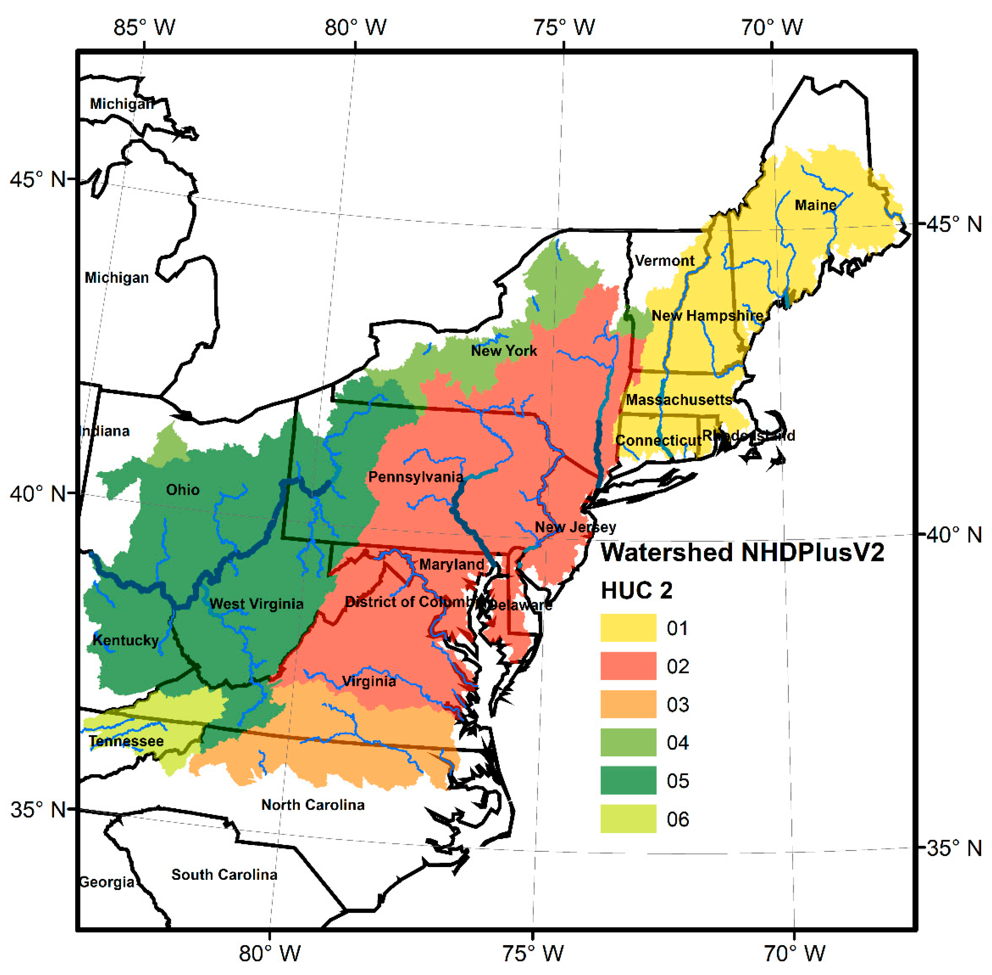
The study area (Figure 1) corresponds to the northeastern portion of the US, with the southern border extent at approximately 34.59° latitude, and the western border at approximately −87.53° longitude. More than sixty-four million people live in the Northeast of the US near to the east coast, one of the most developed areas in the world. According to the Third National Climate Assessment report [6], the built and natural environment has shown considerably vulnerability to climate hazards and other stresses, with aging infrastructure that has already suffered from climate events related to heat waves and coastal and riverine floods.
3. Methods and Data
We used the WRF-Hydro framework as our hydrological model to estimate changes in the terrestrial hydrology from 1980 to 2015 using settings similar to the experimental version implemented in the National Flood Interoperability Experiment [19,20,21]. We evaluated the performance of the model by comparing streamflow calculations to observations by the US Geological Survey (USGS). Moreover, we studied how precipitation gets distributed between the storage (snow accumulation, soil moisture, liquid and frozen water at the canopy) and the outputs of the system (evaporation, transpiration, surface and subsurface runoff), or Input = Accumulation + Outputs. The North American Land Data Assimilation System (NLDAS-2) climate forcing data was used to feed the hydrological model, and the river routing was done using the Routing Application for Parallel Computation of Discharge (RAPID) model. For the calibration of the model and basin selection for the water budget tendency study, we used the USGS Geospatial Attributes of Gages for Evaluating Streamflow II (Gages II) streamflow observations.
3.1. North American Land Data Assimilation System (NLDAS-2)
The North American Land Data Assimilation System (NLDAS-2) was used to force the WRF-Hydro model. NLDAS-2 has a resolution of 1/8th-degree grid spacing, hourly timing, and ranges from 1 January 1979 to present (accessed on 29 January 2018: https://ldas.gsfc.nasa.gov/nldas/NLDAS2forcing.php). Of the 16 fields in each forcing file, Noah-MP requires nine fields: downward longwave and shortwave radiation (bias corrected), U/V 10-m wind components, 2-m air temperature, and specific humidity, surface pressure, and total precipitation. The non-precipitation forcing inputs were primarily derived from the National Centers for Environmental Prediction (NCEP) North American Regional Reanalysis (NARR) (accessed on 29 January 2018: http://www.emc.ncep.noaa.gov/mmb/rreanl/). Precipitation is a product of a temporal disaggregation of a gauge-only Climate Prediction Center (CPC) analysis of daily rainfall performed directly on the NLDAS grid, including an orographic adjustment based on the widely-applied Parameter elevation Regression on Independent Slopes Model (PRISM) climatology. We used an National Center for Atmospheric Research (NCAR) common language (NCL) code provided by the WRF-Hydro research group to further interpolate the forcing data to the hydrology model resolution of 3 km (accessed on 29 January 2018: https://ral.ucar.edu/projects/wrf_hydro/regridding-scripts).
3.2. WRF-Hydro Model
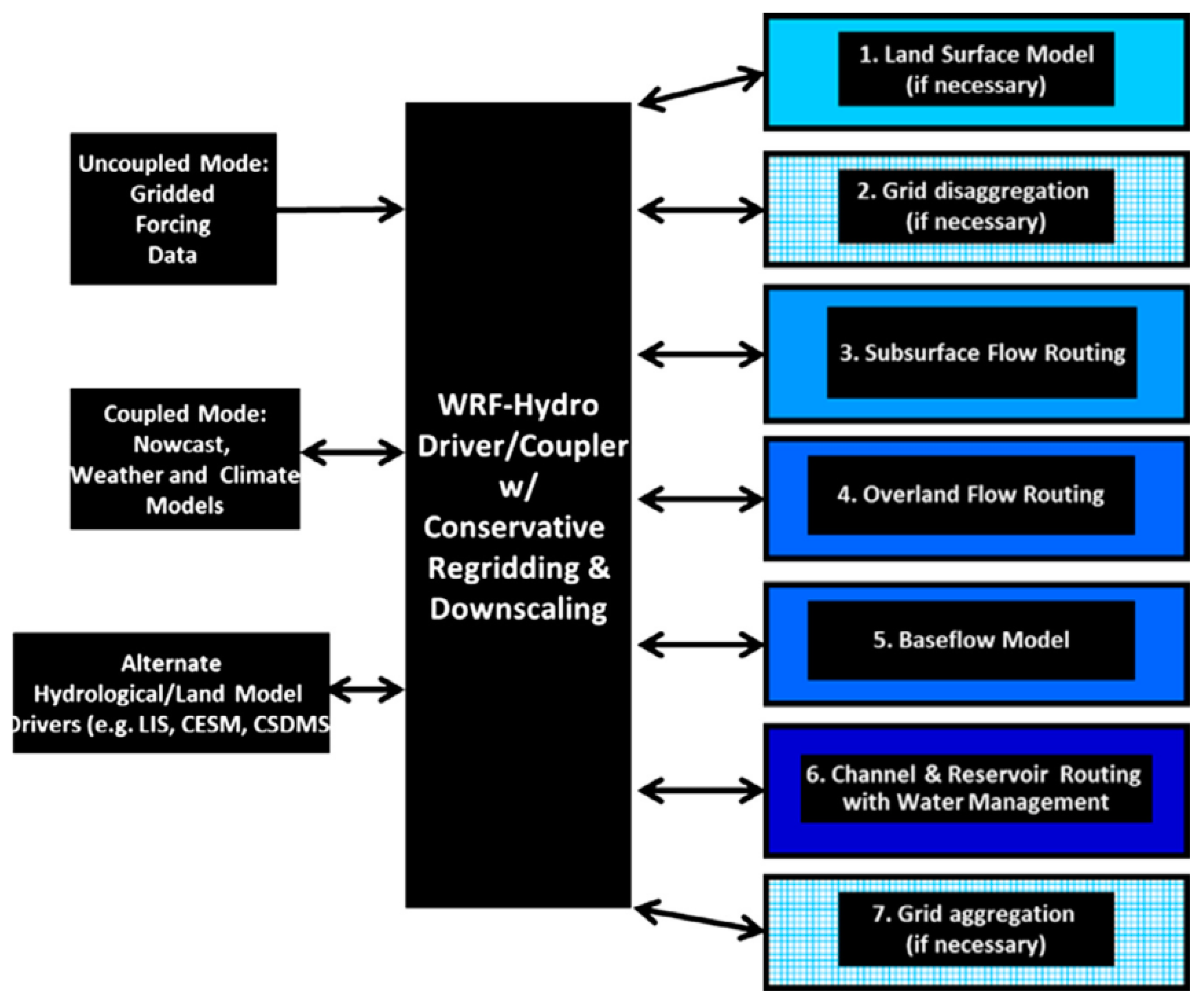
We used the Weather Research Forecast Hydro extension version 3 (WRF-Hydro V3) [22] to calculate runoff. The WRF-Hydro modeling system allows the coupling of hydrological model components to an atmospheric model. The WRF-Hydro configuration (Figure 2), at the highest level, can work in two modes: coupled and uncoupled to an atmospheric model. It then provides the architecture to select among different Land Surface Models (LSM), such as Noah and Noah with multi-parameterization (MP) (hereafter Noah-MP), to solve the energy and mass balance in one-dimensional vertical land surface parameterization. Noah LSM, which has a long history of development in coupled and uncoupled to climate models, is the base for Noah-MP, which allows the user to select among multiple physics option that enables further experimentation, or to generate ensemble results without altering the code [23]. In WRF-Hydro, on the other hand, the user can select from several physic options, such as surface overland flow, saturate subsurface flow, channel routing, and reservoir routing, that provide lateral water transport that allows leaving the one-dimensional column setting. We used the WRF-Hydro uncoupled from the WRF model configuration. For the LSM, we used the Noah-MP [23,24] model. In our case, we selected the physics indicated in Table 1 For the hydronamelist, which controls the horizontal movement of the water, we only kept active the bucket groundwater module with exponential parameters that we used for calibration [22].
3.3. National Hydrography Dataset Plus Version 2 (NHDplusV2) and RAPID
Although WRF-Hydro V3 is capable of routing the water through a river network, it is computationally expensive. Therefore, once we had the runoff (surface and subsurface) from WRF-Hydro, we used the RAPID model to route the water through the National Hydrological Dataset river network [25]. Similar work is described in David et al. [25,26], Salas et al. [19], and Lin et al. [27]. The RAPID model, which is very efficient and able to run on a personal computer, uses the well-documented Muskingham method, which relies on two coefficients that are used to represent the travel time and attenuation of flood waves, K, and X, respectively. The study area corresponds to the hydrology regions Northeast, Mid-Atlantic, the northern part of the South Atlantic region, and the eastern part of the Ohio region (Visited 2 January 2018: http://www.horizon-systems.com/NHDPlus/NHDPlusV2_data.php). RAPID needs two datasets: static and dynamic. The static dataset corresponds to the network topology described in a series of comma separated values (CSV) files that indicates how the streamlines in the river network are connected, as well as the X and K parameters for each line [26]. In the domain study, we used 324,746 flowlines with a mean length of 1.589 km and a standard deviation of 1.45 km; therefore, we can calculate streamflow in 324,746 points. The second dataset corresponds to the runoff derived, in our case, from WRF-Hydro. The land surface model operates in a gridded domain, while RAPID runs in a lumped domain. To transform the data from one domain to the next, we used a simple weighting process that allowed us to calculate the contribution of runoff to each catchment unit. This process and the tools are described by Lin et al. [28] and Salas et al. [19]. We used 318,026 catchments, with an average area of 2.13 km2 and a standard deviation of 3.07 km2.
3.4. Streamflow Data, Calibration, and Spin-Up
To evaluate our streamflow calculation, we used the Geospatial Attributes of Gages for Evaluating Streamflow, version II (Gages II). The U.S. Geological Survey (USGS) maintains this dataset that consists of at least 20 complete years of streamflow (not necessarily consecutive) from 1950 to 2009. Within the Gages II, there is a group of 742 gages denominated as a reference that can be used for hydroclimatic studies since they belong to watersheds with minimal disturbance, having less than 5 percent imperviousness as measured from the National Land Cover Database (NLCD) 2006. (Visited 2 January 2018: https://water.usgs.gov/GIS/metadata/usgswrd/XML/gagesII_Sept2011.xml). From this national dataset, in the area of study, there are 1717 USGS streamflow Gages II, from this number 402/1315 correspond to reference/no-reference watersheds, respectively. Since our analysis runs from 1979 to 2015, we selected 1093 Gages II that have at least 15 years of data for the period of our work. From these 1093 gages, 191 are reference gages, and 902 are non-reference gages.
The spin-up process was carried out following Cai et al. [29] for initializing Noah-MP by running the model 50 times through the entire year of 1979. WRF-hydro, compared to other hydrology models, is computationally expensive; therefore, the number of runs to calibrate the model were limited. Additionally, manual calibration was not desirable because of the number of parameters that need to be adjusted in the model made the manual procedure impractical [30,31]. For these reasons, we calibrated the model using just one year of results from 1980. We ran the model 500 times using a Monte Carlo Markov Chain data parameter estimation as part of the Statistical Parameter Optimization Tool in Python l (SPOTPY), which is a ready-made python package [32], similar to the Model-Independent Parameter Estimation (PETS) that was used in Senatore et al. [33] to calibrate WRF-Hydro. The procedure followed is identical to previous work by References [30,31,33]. The variables used in this calibration were infiltration factor (REFTKD) between 0.5–5 [34], and SLOPE, which is a coefficient between 0.1–1.0 that modifies the drainage out of the bottom of the last soil layer. A larger surface slope implies more considerable drainage [35], saturated soil hydraulic conductivity (DKSAT) [35], and an exponential coefficient within the bucket model within WRF-Hydro/Noah-MP. For the routing using the RAPID model, we included in the calibration the K and X parameters. To reduce the influence of false and unusually extreme values, we smoothed the streamflow using a 5-day rolling average [16,36,37]. In the calibration process, we compared the streamflow results simultaneously at 191 USGS stream Gages II reference locations, minimizing the square distance sum between the Kling–Gupta efficiency (KGE) (Equation (1)) [38] and the perfect value of 1.
where:
r = correlation coefficient, mean value of simulation/observation, standard deviation of simulation/observation.
There are multiple indicators to evaluate the quality of the results in the calibration/evaluation period, depending on the application of the results (i.e., calculation of high or low flows) [39]. Nash Sutcliffe efficiency (NSE) (Equation (2)), percentage bias (PCbias) (Equation (3)), and the ratio of the root mean square error to the standard deviation of measured data (RSR) (Equation (4)) are the most used. Moriasi et al. [40] concluded that, in general, models with monthly NSE > 0.5, RSR < 0.70, and PBIAS ± 25% represent streamflow satisfactorily.
3.5. Changes in Streamflow
Multiple methodologies are available to determine changes in streamflow, i.e., the center of mass that indicates the timing for when half of the water passes, the time of the peak flow, 3-day peak flow for large events analysis [37,41,42,43] or 7-day low flow to characterize water quality, and ecosystems impacts [37,44,45]. A more robust technic that can apply to different hydrological regimes is presented in Reference [36]. This method assessed monotonic trends in time series of 5-day means. Using a 5-day period allows users to obtain similar hydrological responses in both small and large watersheds [36], and to remove the effect of short-term anomalous oscillations [37,46]. This approach reveals runoff timing changes throughout the entire year, whereas other methods focus on a single annual event, or a specific month or season [36]. In this work, we used three metrics, i.e., monthly 3-day peak flow (Q3), monthly 7-day low flow (Q7), and monotonic 5-day means (5) trends, to determine the effects of climate change in streamflows. The first two metrics are straightforward: For the Q3, we used a 3-day moving average and selected the maximum value for each year; for the Q7, we used a 7-day moving average and selected the minimum value for each year. For the 5, we normalized streamflow by subtracting their annual mean and dividing by their standard deviation; then we calculated 73 5 each year, and for each of the 73 time series, the slope of the Kendall-Theil robust line [36].
3.6. Water Budget
The water budget is the relationship between the water inputs, outputs, and accumulation in a hydrological system. Understanding the tendencies in water budget provide information on how changes in temperature and precipitation change the timing of accumulation, evaporation, and streamflow in a specific location. Several studies have focused on the changes on snow/precipitation partition [3], changes in the timing of streamflow [37], changes on snowpack [15], among others.
We calculated the tendencies in the water budget on an annual basis, as well as on a monthly basis, to understand the redistribution of water outputs and accumulation within the year.
where:
Precipitation = Output + Accumulation
Precipitation = solid + liquid rainfall
Output = evaporation + transpiration + surface + subsurface runoff
Accumulation = snow accumulation + soil moisture + liquid and frozen water at the canopy.
4. Results
We ran WRF-Hydro from 1979 to 2015 with three goals in mind: (1) to provide a consistent hydrology model dataset for 37 years across the area of study; (2) to evaluate in the long term the performance of the model in this region; and (3) to learn about the tendencies in the water budget component during the last four decades in the Northeast of the US.
4.1. Performance of the Model
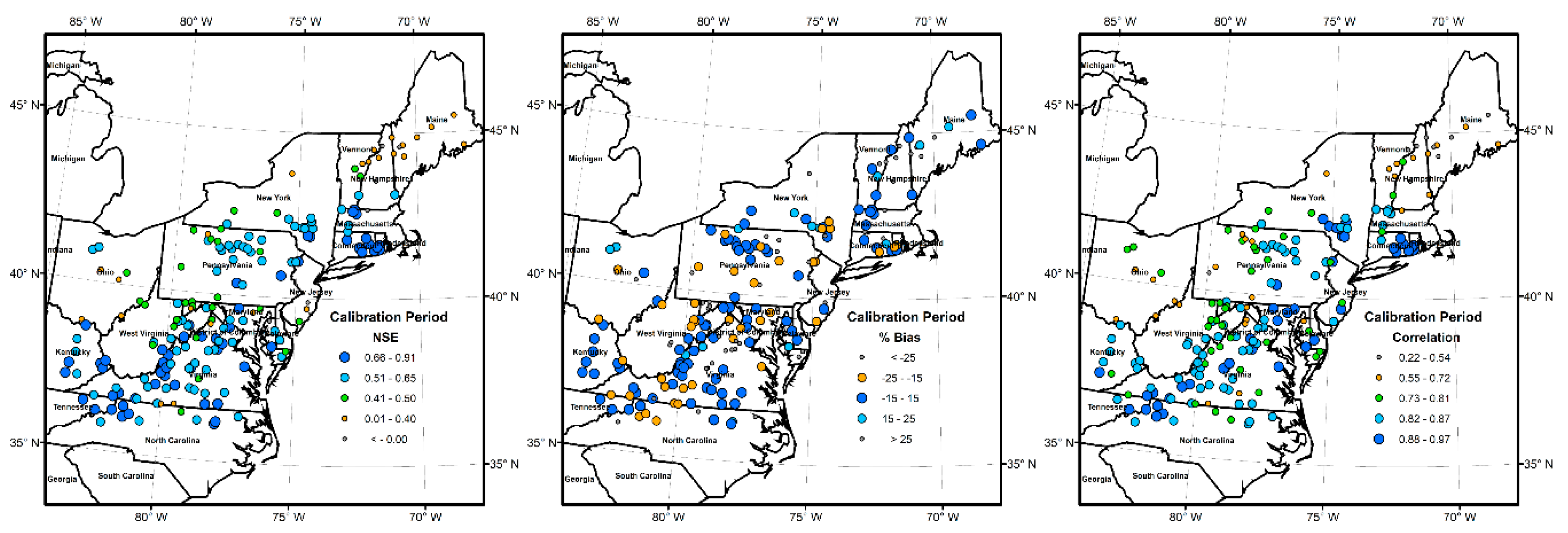
After running the model 50 times to spin-up the system, we used the restart files to calibrate WRF-Hydro and RAPID for the year 1980. We compared the daily streamflow time series for 191 USGS Gages II references for the area of study. The calibration results indicated that the model results obtained NSE > 0.5 for 136 stations and NSE > 0.4 for 160 stations. One hundred forty-six stations had a |PBias| < 25%, and 96 had a |PBias| < 15%. For RSR, 133 stations had an RSR < 0.7 (Figure 3).
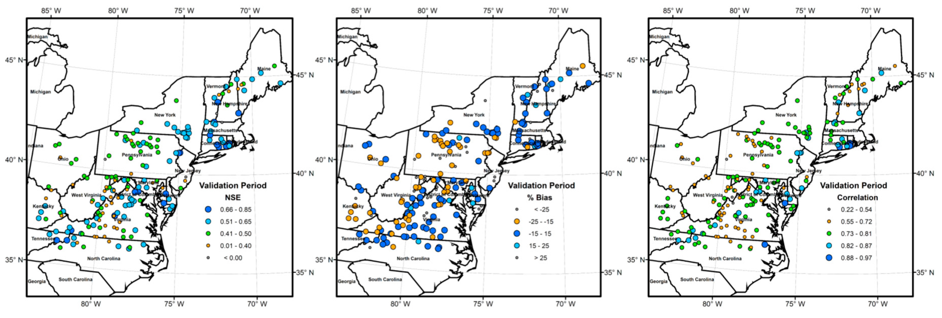
For the validation period (1981–1990), the general performance of the model slightly decreased, although it still showed satisfactory results in stream gages covering the entire study area. The model results obtained NSE > 0.5 for 92 stations and NSE > 0.4 for 152 stations. One hundred fifty-four stations had a |PBias| < 25%, and 90 had a |PBias| < 15%. For RSR, 91 stations had an RSR < 0.7 (Figure 4).
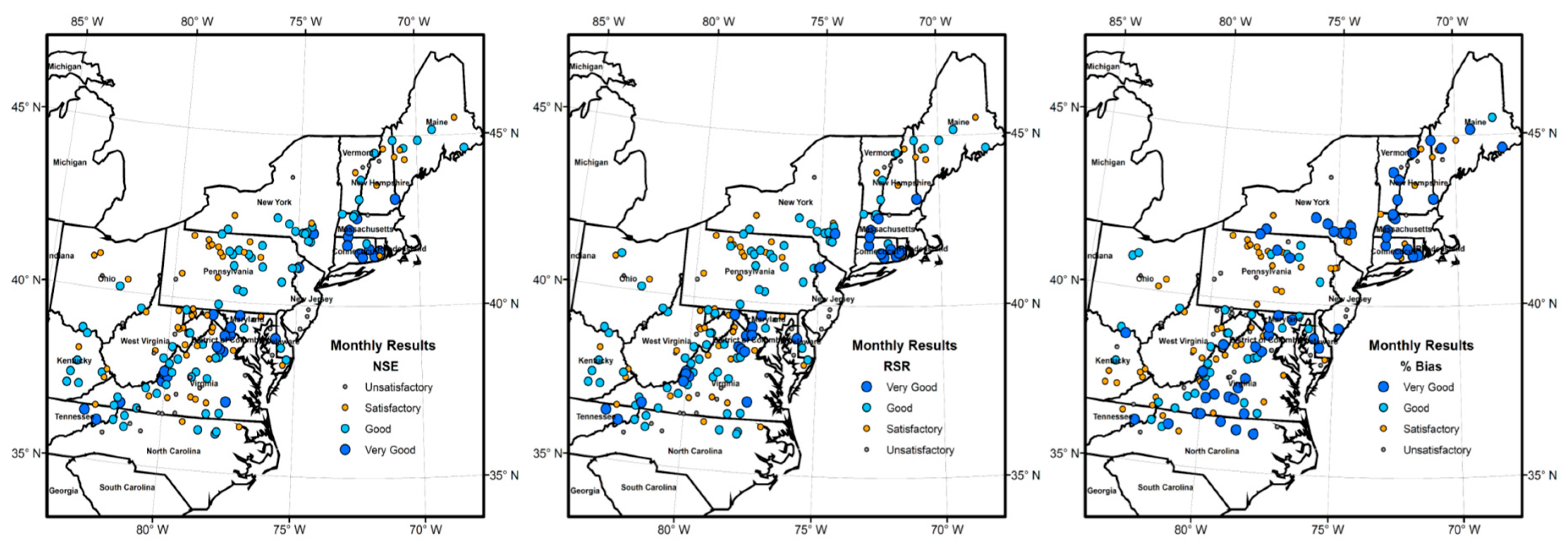
In Figure 5, we also show the performance of the model for monthly values for the period 1980 to 2015, using the nomenclature of Reference [40]. For NSE, 30 stations were very good, 77 stations were good, 55 were satisfactory, and 27 stations were unsatisfactory. For RSR, 30 stations were very good, 83 stations were good, 50 were satisfactory, and 26 stations were unsatisfactory. Finally, for PBias, 61 stations were very good, 34 stations were good, 61 were satisfactory, and 33 stations were unsatisfactory.
4.2. Changes in Streamflow and Water Budget Components
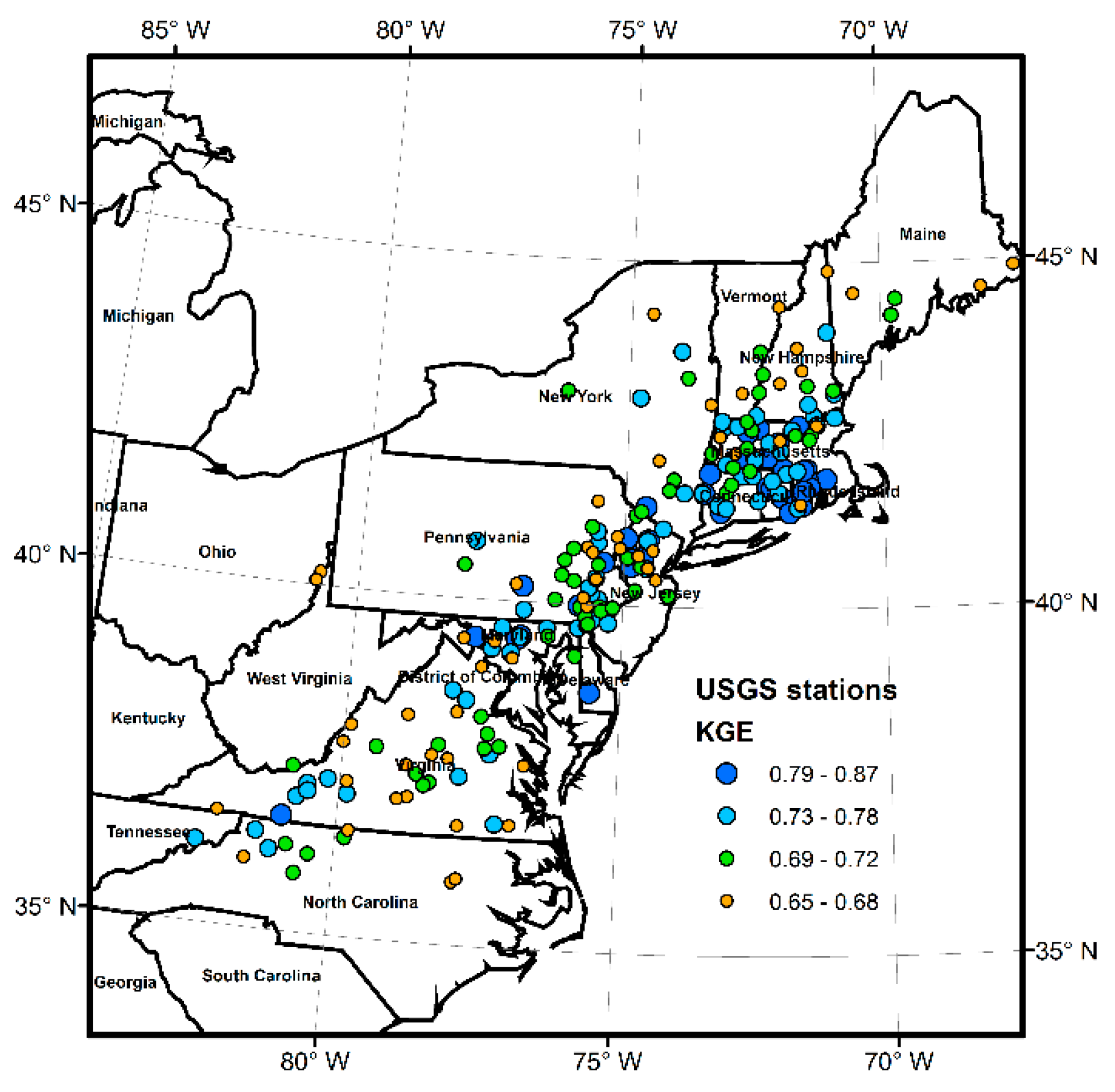
Considering the extent of our model, we increased the number of basins in which we did our analysis by comparing our results to 889 USGS Gage II references and non-references. From these 889 points, we selected the 242 points where our model’s results have a KGE above 0.65 for 35+ year time series; Figure 6 shows their geographical distribution. We estimated tendencies for Q3, Q7, and 5, and the water budget component (input, output, and accumulation) tendency. For the streamflow, we aggregated the result in three categories by area and three categories by latitude. With the former, we wanted to know if larger watersheds can reduce the effects of climate change, while the latter was designed to estimate if there is a south-north tendency gradient in the streamflow. We did this for the model results, as well as for the USGS observations, to show the ability of the model to capture such trends.
4.2.1. Three-Day Peak Flow (Q3)
The model overestimated the tendencies for Q3 (Figure 7); however, it could capture the general behavior of the changes. When we separated the results by latitude, the Q3 behaved similarly from south to north; however, when we compared by area, we could see that we had a result similar to Chezik et al. [16] since larger surfaces can buffer or reduce the effects of climate variability and do not show extreme changes (on average) compared to small catchments. The Q3 flows increased more during the late summer and early autumn for basins with areas lower than 250 km2.
4.2.2. Seven-Day Low Flow (Q7)
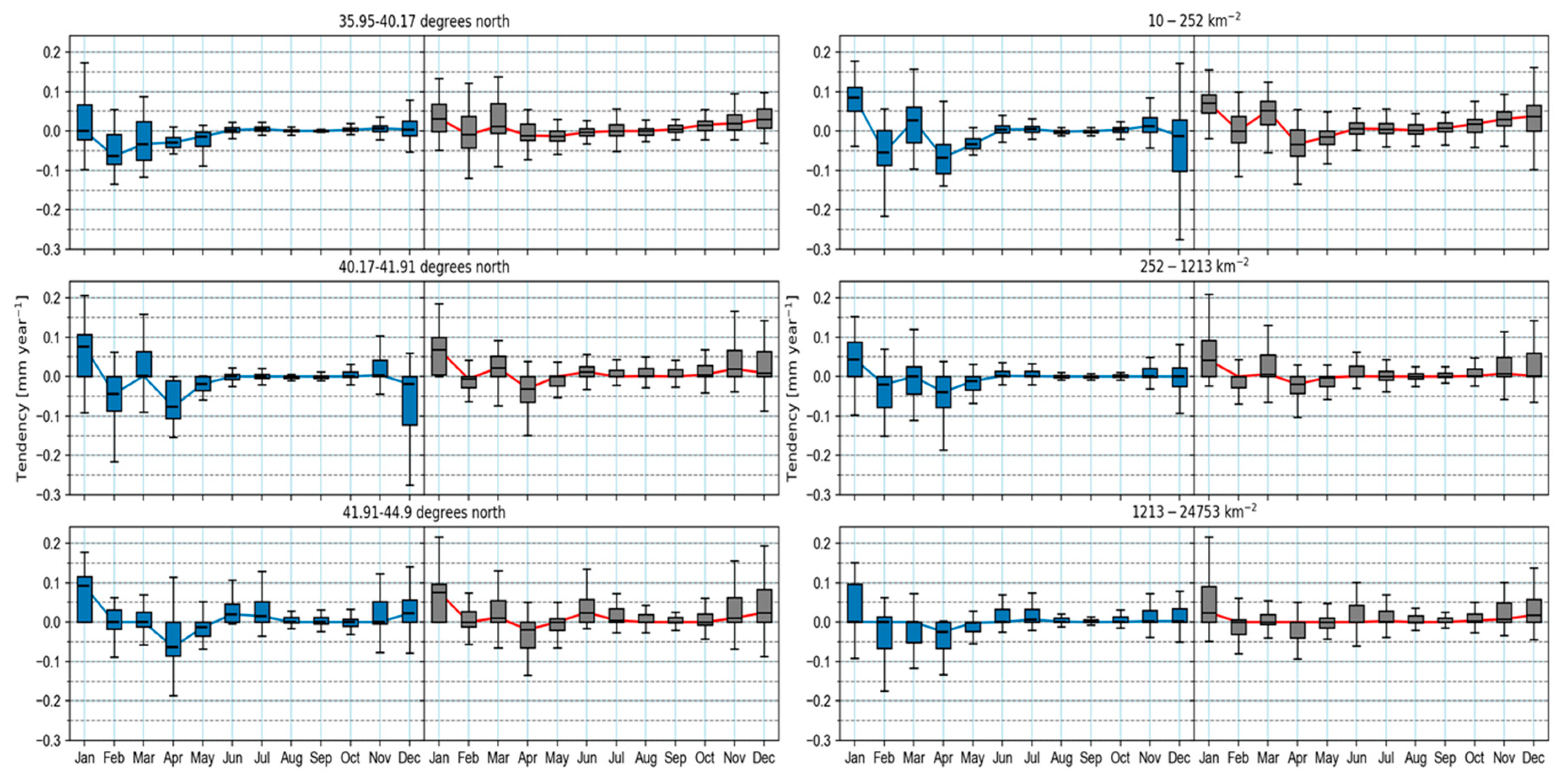
Trends in the observed and modelled results indicate there were more substantial changes in the Q7 for winter, especially for small catchments (Figure 8). We observed that larger basins had lower trends; although, in general, the trends indicated that, on average, there was an increase in low flows, with a favorable north-south gradient that coincided with the annual Q7 tendencies reported by Kam and Sheffield [18]. April was the only month that presented negative trends, which were captured in the model results. However, the model also estimated negative trends for February in middle and southern latitudes, which did not match the observations.
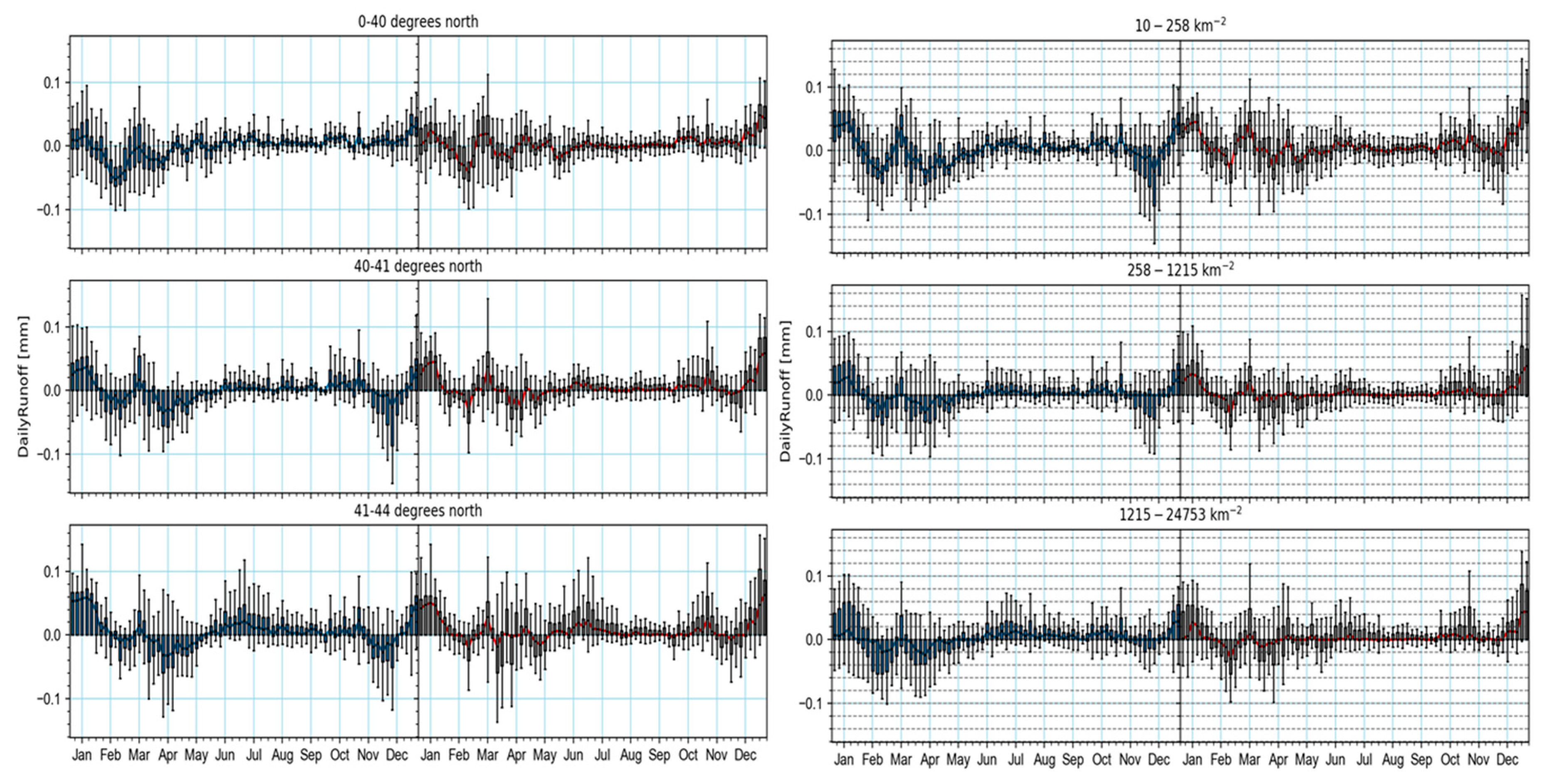
4.2.3. Five-Day Means (5)
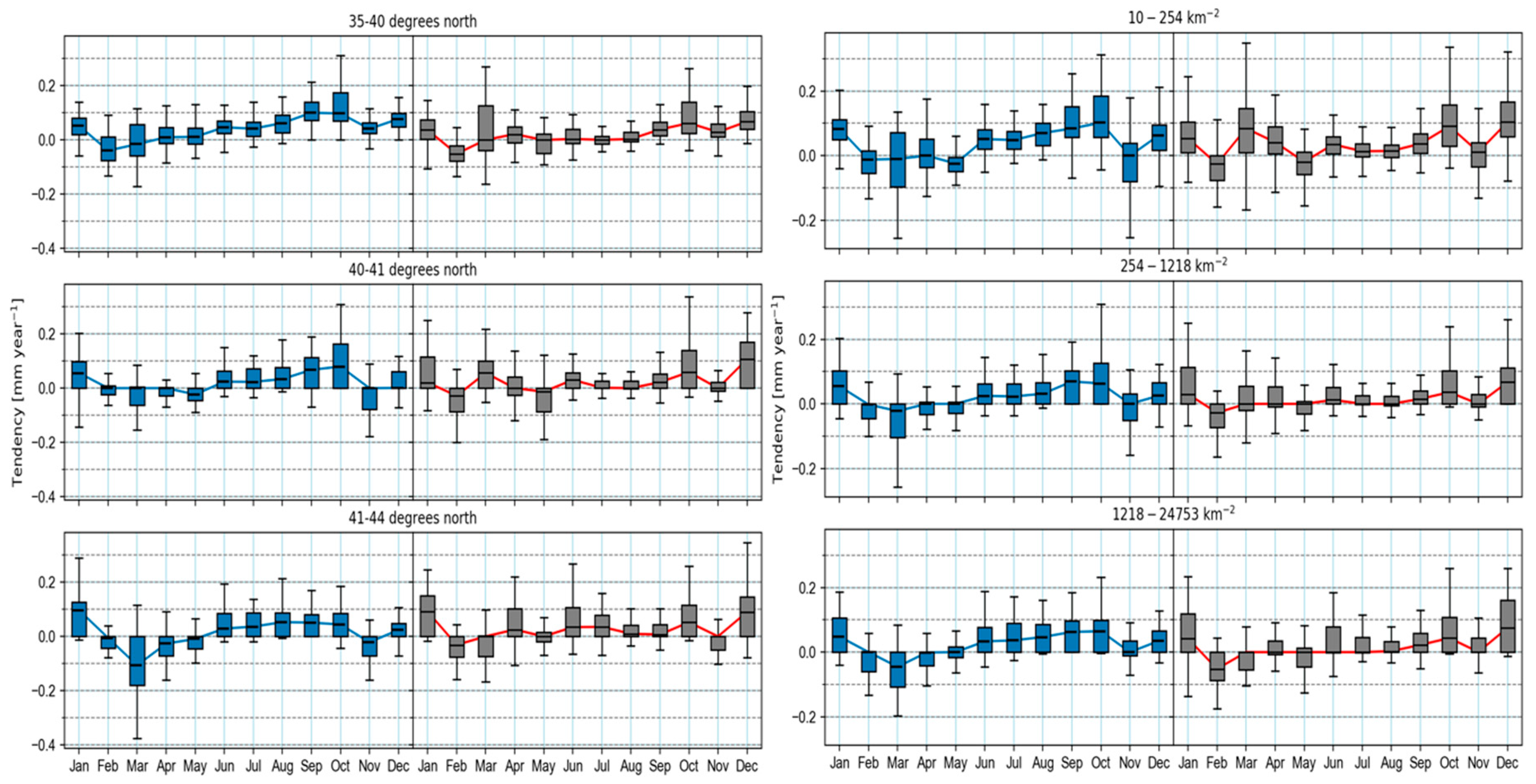
The model compared very well with the USGS observations for the 5 (Figure 9). We identified two major regions of change in streamflow: The first occurs during the months of November, December, and January, when streamflow volumes have increased, with an abrupt drop around February. These increases were larger in the northern basins, with the opposite happening during the February drop. We then identified that smaller basins had larger fluctuations in trends during the spring which were attenuated as the basin areas increased. Finally, basins located further north had more available water during the summer, but in general, the analysis indicated that more water was available through the year, except for the middle of the spring. The model also showed that there was a negative trend around April for middle and northern latitudes, which was not detected in the observations; however, this seemed to be due to a large negative trend that the NLDAS-2 precipitation had in the same month (Figure 10a).
4.3. Water Budget
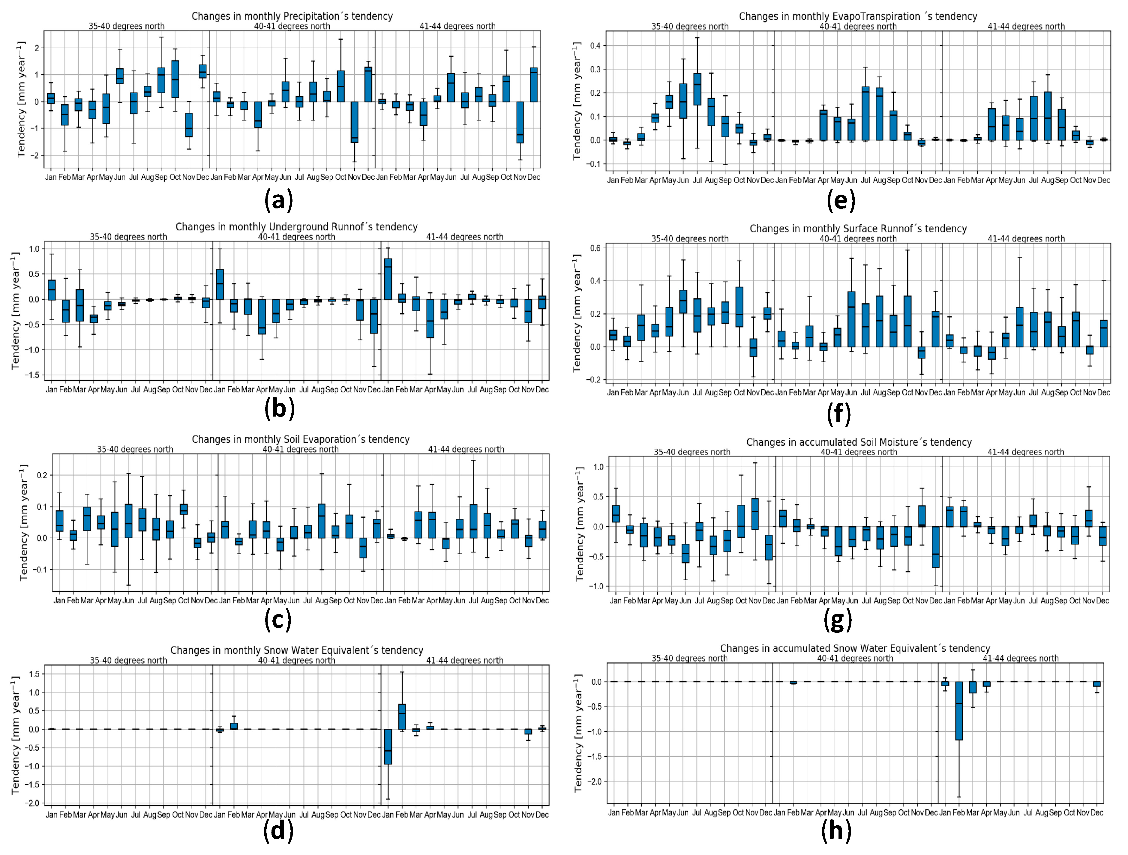
WRF-Hydro results were cumulative for the component of the water budget. Therefore, to obtain changes in a month, we had to subtract from the last day of the month when analyzing the results for the last day of the previous month. The water budget calculation used is as follows: the balance inputs = outputs + accumulation. The input in this study was precipitation (liquid and solid) corresponding to NLDAS-2 total precipitation, which originally drove the hydrological model (Figure 10a). The outputs were evapotranspiration (ET) (Figure 10e), surface runoff (Figure 10f), underground runoff (Figure 10b), and bare soil evaporation (Figure 10c). Finally, the accumulation was represented by canopy water content (liquid and frozen), which was not shown here because was very small, soil moisture (Figure 10g), snow water equivalent (SWE) monthly accumulations (Figure 10d), and SWE total accumulation (Figure 10h). When we calculated the annual water balance, the accumulation tended toward zero, which was expected and desired from the model.
Precipitation tendencies were mixed, with positive larger tendencies occurring during the summer and fall, except for November, and negative tendencies occurring during the middle of the winter to the middle of the spring, showing a clear change in the distribution of the precipitation toward the warmer seasons. Because of this, more water was available for evapotranspiration for the warmer months, which showed that there was a positive trend in most of the catchments to produce more evapotranspiration. For the runoff, there was a change in the fraction of runoff that went underground or stayed at the surface. Underground runoff decreased almost the entire year, except during January when less snow was accumulated and there was probably more water available to infiltrate. On the other hand, surface runoff increased, except for the early spring in mid-latitudes, which is explained by a reduction in precipitation, but the tendencies suggested that the increase in precipitation during the warm months went mostly to surface runoff. This change was also suggested by the tendencies in soil moisture that decreased for most of the year, which was a consequence of larger canopy evapotranspiration and soil evaporation and lower infiltration. For the SWE, we present two plots in Figure 10 (bottom row), the plot at the left showing the tendency for the total accumulated snow, which decreases for the entire season. The plot at the right shows the tendencies in the monthly accumulation for what we estimate to be the changes in snow accumulation during the month. The months where the trends are negative are straightforward for interpretation as a reduction in the snow accumulated during that month. However, in the months with positive trends, there is a mix of processes that explain the trend. First, the snow falls also decreased (less total precipitation and higher temperatures); however, what made it positive was that in those months when the snow started melting, there was less snow to melt due to the accumulation deficit from the previous month. Therefore, the normal negative changes in accumulation were reduced.
5. Discussion
5.1. Model Performance
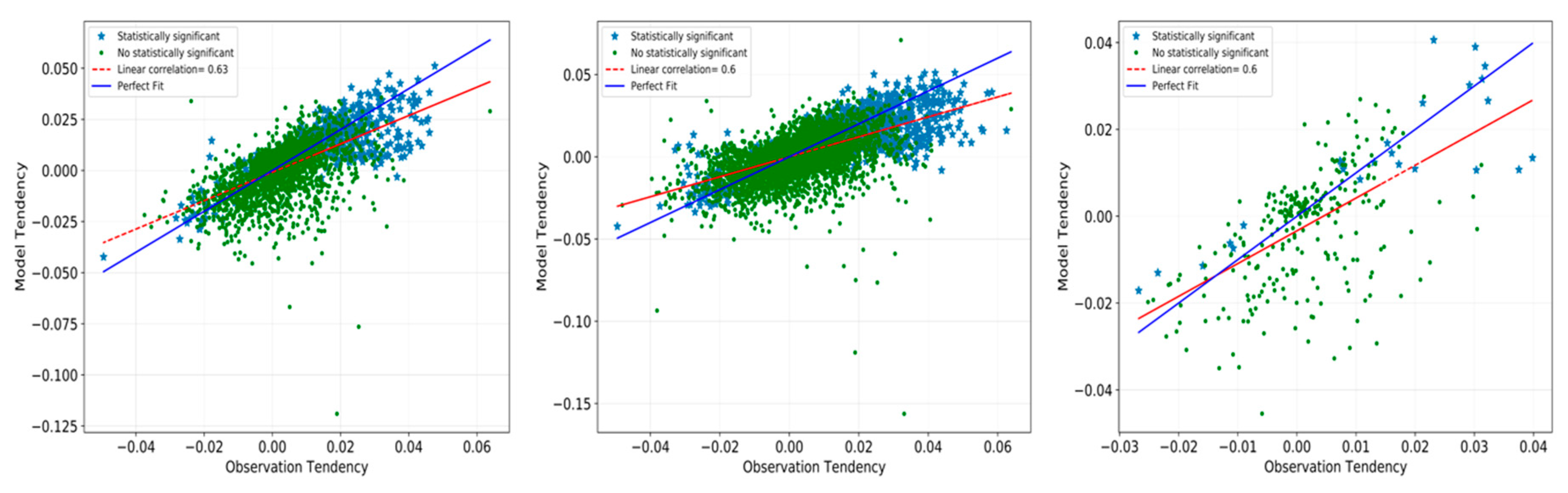
The model has good results across the domain of study, with better statistic scores for monthly streamflow than smoothed daily streamflow. The model performance, according to traditional standards [40], for 150 out of 191 stations is considered at least satisfactory for the validation period for smoothed daily values, and 160 stations are at least satisfactory for monthly results. However, when it comes to determining streamflow trends, the traditional performance evaluation criteria do not ensure that the model will capture well the slope of the trends. The dispersions around the perfect line in Figure 11 are not described by NSE, PCBias, correlation, or KGE, which are also dependent on the extent of the dataset, in our case 36 years. Therefore, there is a need to come up with a calibration metric that includes the estimation of the trends which are a common indicator to describe climate change. For example, in Figure 11, we plot the results filtered by KGE. The left graph shows the tendency values for KGE > 0.65, the middle KGE > 0.5, and the right KGE > 0.8. However, the correlation between the tendency for observation and the model are 0.66, 0.6, and 0.6, which indicates that having a better KGE does not imply that we will have a better estimation of the trend. What it is consistent is that positive larger trends are more often statistically significant (p < 0.05) than trends near zero, which are the majority of the trends.
5.2. Streamflow Tendency
To evaluate the tendencies of streamflow, we use three metrics: monthly three-day peak flow (Q3), monthly seven-day low flow (Q7), and five-day means (5). Q3 is a good indicator for peak flow and therefore useful for flood assessments; Q7 is a good indicator of low flows tendencies that can be useful in water management and ecological applications; and 5 is a good indicator of the changes, shifting in time and amplitude, of streamflow during a year. The three indicators increase during the winter months, which is a consequence of less solid precipitation, despite total precipitation increasing for that period. Our model results capture well the direction of changes during the last 40 years; however, it has a positive bias in the trends calculated for the summer Q3. Q3 also increases for the whole region in the month of October, which may be a consequence of tropical storms moving further north as a consequence of climate change during that period. The Northeast has experienced serious catastrophes in the late summer to early fall, with tropical storms and even hurricanes crossing the region. Small basins also experience an increase in high flows at the beginning of spring. Q7, on the other hand, has slightly increased, with a more pronounced augmentation in the winter. Q7 also has a major increase in March for small basins, which is not the case for larger basing, which suggests that, in the Northeast, larger basins can circumvent the effects of short term rainfall associated with climate change, which is similar to what Reference [16] found on the West Coast. For 5, the most significant positive trends are found in the winter, which can be observed in a reconstruction of the hydrographs for the years 1981 and 2015 (Figure S1). We use the Kendall-Theil slope and intercept to create the hydrographs and see what the differences are in streamflow between 1981 and 2015. In the hydrographs for 1981, we can clearly see that after mid-November, the streamflow decreases, which is due to the fact that, at the time, the solid precipitation fraction was larger; however, if we plot what would happen 34 years later, following the Kendall-Theil slope, the streamflow continues to increase until January, and then drops dramatically in February. Also, for 5, abrupt oscillations in tendencies decrease as the basins get larger.
5.3. Water Budget Tendencies
NLDAS-2 precipitation indicates that there is a positive tendency, which means that there is more water input in the Northeast region of the US. However, the extra water entering the system is not being distributed evenly among the output and accumulation component of the water budget. Streamflow volumes are increasing for most of the year, except for the end of winter, which is a consequence of less snow accumulation during the winter, and in November, which is the result of a decrease in precipitation in late fall. Therefore, in general, there is more water running in the rivers; however, the partition between underground runoff and surface runoff is altered. It seems that underground flow tends to decrease while surface runoff increases for most of the year. This translates to faster responses from the basins, which means that the concentration-time of the water reduces. This is the result of more intense rain that does not have enough time to infiltrate, which is suggested by the fact that soil moisture also decreases for most of the year. Hence, the soils can hold more water. The decrease in underground runoff is also enhanced by more canopy evapotranspiration and soil evaporation due to the increase in temperatures, which is more dramatic in southern latitudes. SWE volume decreases, while the accumulation season gets shorter. This translates into a decrease in spring runoff in the north portion of the study area where basins rely on snow accumulation to supply fresh water in spring.
In the construction of WRF-Hydro model, we did not include changes in land cover, which could be significant in 40 years of natural [47] and anthropogenic disturbances. Therefore, the trends reported here are only based on changes in climate from 1979 to 2016.
6. Conclusions
In this study, we present the application of the WRF-Hydro framework to estimate changes in the water budget for the last 40 years in the Northeast of the US. The model, when compared to streamflow, performs at least satisfactorily for most of the region, capturing aggregated tendencies and comparing well when we use traditional criteria to compare model and observations.
Changes in climate during the last 40 years has brought a redistribution of the water from precipitation within the different components of the water budget at the surface in the Northeast of the US. High, low and medium flow tendencies are mostly positive. Therefore, there is more water available. However, these changes are not evenly distributed during the year, nor between basins of different latitudes. More water is available during winter, but less during the spring. This is a consequence of the decrease in snow accumulation due to temperature increases in the north, and a decrease in precipitation in the south during the second half of the winter.
Although soils are becoming drier, infiltration is decreasing, so the surface runoff is increasing, and therefore, the time of responses of the watersheds are decreasing. Evapotranspiration is also increasing, which will produce more losses from the soil moisture, and less water in the subsurface is available for subsurface runoff or depth infiltration, affecting the storage during the year.
Finally, the effects of climate change in high and low flows seem to be smaller in larger basins. Therefore, efforts to mitigate the impacts of extreme events should be emphasized in smaller watersheds.
Supplementary Materials
The following are available online at https://www.mdpi.com/2073-4441/10/12/1709/s1, Figure S1: Synthetic hydrographs for 1981 (Blue) and 2015 (Red) for area and latitude.
Author Contributions
Conceptualization, M.A.S.-V.; formal analysis, M.A.S.-V.; investigation, M.A.S.-V.; methodology, M.A.S.-V.; resources, R.N.P.; writing—original draft, M.A.S.-V.
Funding
The project described in this publication was supported by Grant or Cooperative Agreement No. G12AC00001 from the United States Geological Survey. Its contents are solely the responsibility of the authors and do not necessarily represent the views of the Northeast Climate Adaptation Science Center (NECASC) or the USGS. This manuscript is submitted for publication with the understanding that the United States Government is authorized to reproduce and distribute reprints for Governmental purposes.
Acknowledgments
We thank the NECASC, specifically we would like to thank T. L. Morelli, A. R. Holland, M. Staudinger and J. Brown for their constant support, and the graduate fellows for their feedback and continuous engagement in interesting research.
Conflicts of Interest
The authors declare no conflict of interest, and the funders had no role in the design of the study, in the collection, analyses, or interpretation of data, in the writing of the manuscript, or in the decision to publish the results.
References
- Karmalkar, A.V.; Bradley, R.S. Consequences of Global Warming of 1.5 °C and 2 °C for Regional Temperature and Precipitation Changes in the Contiguous United States. PLoS ONE 2017, 12, e0168697. [Google Scholar] [CrossRef] [PubMed]
- Berton, R.; Driscoll, C.T.; Chandler, D.G. Changing climate increases discharge and attenuates its seasonal distribution in the northeastern United States. J. Hydrol. Reg. Stud. 2016, 5, 164–178. [Google Scholar] [CrossRef]
- Hayhoe, K.; Wake, C.P.; Huntington, T.G.; Luo, L.; Schwartz, M.D.; Sheffield, J.; Wood, E.; Anderson, B.; Bradbury, J.; DeGaetano, A.; et al. Past and future changes in climate and hydrological indicators in the US Northeast. Clim. Dyn. 2007, 28, 381–407. [Google Scholar] [CrossRef]
- Dudley, R.W.; Hodgkins, G.A.; McHale, M.R.; Kolian, M.J.; Renard, B. Trends in snowmelt-related streamflow timing in the conterminous United States. J. Hydrol. 2017, 547, 208–221. [Google Scholar] [CrossRef]
- Groisman, P.Y.; Knight, R.W.; Karl, T.R. Heavy precipitation and high streamflow in the contiguous United States: Trends in the twentieth century. Bull. Am. Meteorol. Soc. 2001, 82, 219–246. [Google Scholar] [CrossRef]
- Horton, R.; Yohe, G.; Easterling, W.; Kates, R.; Ruth, M.; Sussman, E.; Whelchel, A.; Wolfe, D.; Lipschultz, F. Chapter 16: Northeast. In Climate Change Impacts in the United States: The Third National Climate Assessment; Melillo, J.M., Richmond, T.T.C., Yohe, G.W., Eds.; U.S. Global Change Research Program: Washington, DC, USA, 2014. [Google Scholar]
- Bose, A.K.; Weiskittel, A.; Wagner, R.G. A three decade assessment of climate-associated changes in forest composition across the north-eastern USA. J. Appl. Ecol. 2017, 54, 1592–1604. [Google Scholar] [CrossRef]
- Sanders-DeMott, R.; McNellis, R.; Jabouri, M.; Templer, P.H. Snow depth, soil temperature and plant–herbivore interactions mediate plant response to climate change. J. Ecol. 2018, 106, 1508–1519. [Google Scholar] [CrossRef]
- Brin, L.D.; Goyer, C.; Zebarth, B.J.; Burton, D.L.; Chantigny, M.H. Changes in snow cover alter nitrogen cycling and gaseous emissions in agricultural soils. Agric. Ecosyst. Environ. 2018, 258, 91–103. [Google Scholar] [CrossRef]
- Contosta, A.R.; Burakowski, E.A.; Varner, R.K.; Frey, S.D. Winter soil respiration in a humid temperate forest: The roles of moisture, temperature, and snowpack. J. Geophys. Res. Biogeosci. 2016, 121, 3072–3088. [Google Scholar] [CrossRef] [Green Version]
- Patel, K.F.; Tatariw, C.; MacRae, J.D.; Ohno, T.; Nelson, S.J.; Fernandez, I.J. Soil carbon and nitrogen responses to snow removal and concrete frost in a northern coniferous forest. Can. J. Soil Sci. 2018, 12, 1–12. [Google Scholar] [CrossRef]
- Sanders-DeMott, R.; Sorensen, P.O.; Reinmann, A.B.; Templer, P.H. Growing season warming and winter freeze–thaw cycles reduce root nitrogen uptake capacity and increase soil solution nitrogen in a northern forest ecosystem. Biogeochemistry 2018, 137, 337–349. [Google Scholar] [CrossRef]
- Armstrong, W.H.; Collins, M.J.; Snyder, N.P. Hydroclimatic flood trends in the northeastern United States and linkages with large-scale atmospheric circulation patterns. Hydrol. Sci. J. 2014, 59, 1636–1655. [Google Scholar] [CrossRef] [Green Version]
- Armstrong, W.H.; Collins, M.J.; Snyder, N.P. Increased Frequency of Low-Magnitude Floods in New England. J. Am. Water Resour. Assoc. 2012, 48, 306–320. [Google Scholar] [CrossRef]
- Demaria, E.M.; Roundy, J.K.; Wi, S.; Palmer, R.N. The Effects of Climate Change on Seasonal Snowpack and the Hydrology of the Northeastern and Upper Midwest United States. J. Clim. 2016, 29, 6527–6541. [Google Scholar] [CrossRef]
- Chezik, K.A.; Anderson, S.C.; Moore, J.W. River networks dampen long-term hydrological signals of climate change. Geophys. Res. Lett. 2017, 44. [Google Scholar] [CrossRef]
- Hodgkins, G.A.; Dudley, R.W.; Huntington, T.G. Changes in the timing of high river flows in New England over the 20th Century. J. Hydrol. 2003, 278, 244–252. [Google Scholar] [CrossRef] [Green Version]
- Kam, J.; Sheffield, J. Changes in the low flow regime over the eastern United States (1962–2011): Variability, trends, and attributions. Clim. Chang. 2016, 135, 639–653. [Google Scholar] [CrossRef]
- Salas, F.R.; Somos-Valenzuela, M.A.; Dugger, A.; Maidment, D.R.; Gochis, D.J.; David, C.H.; Yu, W.; Ding, D.; Clark, E.P.; Noman, N. Towards Real-Time Continental Scale Streamflow Simulation in Continuous and Discrete Space. JAWRA J. Am. Water Resour. Assoc. 2017. [Google Scholar] [CrossRef]
- Lin, P.; Rajib, M.A.; Yang, Z.; Somos-Valenzuela, M.; Merwade, V.; Maidment, D.R.; Wang, Y.; Chen, L. Spatiotemporal Evaluation of Simulated Evapotranspiration and Streamflow over Texas using the WRF-Hydro-RAPID Modeling Framework. JAWRA J. Am. Water Resour. Assoc. 2017, 40–54. [Google Scholar] [CrossRef]
- Maidment, D.R. Conceptual Framework for the National Flood Interoperability Experiment. JAWRA J. Am. Water Resour. Assoc. 2017, 53, 245–257. [Google Scholar] [CrossRef]
- Gochis, D.; Yu, W.; Yates, D. WRF—Hydro Technical Description and User’s Guide Version 3; Center for Atmospheric Research (NCAR): Boulder, CO, USA, 2015. [Google Scholar]
- Yang, Z.; Cai, X.; Zhang, G.; Tavakoly, A.; Jin, Q.; Meyer, L.H.; Guan, X. The Community Noah Land Surface Model with Multi-Parameterization Options: Technical Description; Center for Integrated Earth System Science, The University of Texas at Austin: Austin, TX, USA, 2011. [Google Scholar]
- Yang, Z.-L.; Niu, G.-Y.; Mitchell, K.E.; Chen, F.; Ek, M.B.; Barlage, M.; Longuevergne, L.; Manning, K.; Niyogi, D.; Tewari, M.; et al. The community Noah land surface model with multiparameterization options (Noah-MP): 2. Evaluation over global river basins. J. Geophys. Res. 2011, 116, D12110. [Google Scholar] [CrossRef]
- David, C.H.; Maidment, D.R.; Niu, G.-Y.; Yang, Z.-L.; Habets, F.; Eijkhout, V. River Network Routing on the NHDPlus Dataset. J. Hydrometeorol. 2011, 12, 913–934. [Google Scholar] [CrossRef] [Green Version]
- David, C.H.; Yang, Z.L.; Hong, S. Regional-scale river flow modeling using off-the-shelf runoff products, thousands of mapped rivers and hundreds of stream flow gauges. Environ. Model. Softw. 2013, 42, 116–132. [Google Scholar] [CrossRef]
- Lin, P.; Yang, Z.-L.; Gochis, D.J.; Yu, W.; Maidment, D.R.; Somos-Valenzuela, M.A.; David, C.H. Implementation of a vector-based river network routing scheme in the community WRF-Hydro modeling framework for flood discharge simulation. Environ. Model. Softw. 2018, 107, 1–11. [Google Scholar] [CrossRef]
- Lin, P.; Yang, Z.; Cai, X.; David, C.H. Regional Studies Development and evaluation of a physically-based lake level model for water resource management: A case study for Lake. J. Hydrol. 2015, 4, 661–674. [Google Scholar] [CrossRef]
- Cai, X.; Yang, Z.; Xia, Y.; Huang, M.; Wei, H.; Leung, L.R.; Ek, M.B. Assessment of simulated water balance from Noah, Noah-MP, CLM, and VIC over CONUS using the NLDAS test bed. J. Geophys. Res. Atmos. 2014, 119, 13–751. [Google Scholar] [CrossRef]
- Givati, A.; Gochis, D.; Rummler, T.; Kunstmann, H. Comparing One-Way and Two-Way Coupled Hydrometeorological Forecasting Systems for Flood Forecasting in the Mediterranean Region. Hydrology 2016, 3, 19. [Google Scholar] [CrossRef]
- Yucel, I.; Onen, A.; Yilmaz, K.K.; Gochis, D.J. Calibration and evaluation of a flood forecasting system: Utility of numerical weather prediction model, data assimilation and satellite-based rainfall. J. Hydrol. 2015, 523, 49–66. [Google Scholar] [CrossRef] [Green Version]
- Houska, T.; Kraft, P.; Chamorro-Chavez, A.; Breuer, L. SPOTting model parameters using a ready-made python package. PLoS ONE 2015, 10, e0145180. [Google Scholar] [CrossRef] [PubMed]
- Senatore, A.; Mendicino, G.; Gochis, D.J.; Yu, W.; Yates, D.N.; Kunstmann, H. Fully coupled atmosphere-hydrology simulations for the central Mediterranean: Impact of enhanced hydrological parameterization for short and long time scales. J. Adv. Model. Earth Syst. 2015, 7, 1693–1715. [Google Scholar] [CrossRef] [Green Version]
- Niu, G.-Y. The Community Noah Land Surface Model (LSM) with Multi-Physics Options, User’s Guide; Center for Integrated Earth System Science, The University of Texas at Austin: Austin, TX, USA, 2011. [Google Scholar]
- Mitchell, K.; Ek, M.; Wong, V.; Lohmann, D.; Koren, V.; Schaake, J.; Duan, Q.; Gayno, G.; Moore, B.; Grunmann, P.; et al. Noah Land Surface Model (LSM) User’s Guide; Noah: Corvallis, OR, USA, 2005. [Google Scholar]
- Déry, S.J.; Stahl, K.; Moore, R.D.; Whitfield, P.H.; Menounos, B.; Burford, J.E. Detection of runoff timing changes in pluvial, nival, and glacial rivers of western Canada. Water Resour. Res. 2009, 45, 1–11. [Google Scholar] [CrossRef]
- Demaria, E.M.; Palmer, R.N.; Roundy, J.K. Regional climate change projections of streamflow characteristics in the Northeast and Midwest U.S. J. Hydrol. Reg. Stud. 2016, 5, 309–323. [Google Scholar] [CrossRef]
- Gupta, H.V.; Kling, H.; Yilmaz, K.K.; Martinez, G.F. Decomposition of the mean squared error and NSE performance criteria: Implications for improving hydrological modelling. J. Hydrol. 2009, 377, 80–91. [Google Scholar] [CrossRef] [Green Version]
- Pushpalatha, R.; Perrin, C.; Le Moine, N.; Andréassian, V. A review of efficiency criteria suitable for evaluating low-flow simulations. J. Hydrol. 2012, 420–421, 171–182. [Google Scholar] [CrossRef]
- Moriasi, D.N.; Arnold, J.G.; van Liew, M.W.; Bingner, R.L.; Harmel, R.D.; Veith, T.L. Model Evaluation Guidelines for Systematic Quantification of Accuracy in Watershed Simulations. Trans. ASABE 2007, 50, 885–900. [Google Scholar] [CrossRef]
- Maurer, E.P.; Adam, J.C.; Wood, A.W. Climate model based consensus on the hydrologic impacts of climate change to the Rio Lempa basin of Central America. Hydrol. Earth Syst. Sci. 2009, 13, 183–194. [Google Scholar] [CrossRef] [Green Version]
- Maurer, E.P.; Brekke, L.D.; Pruitt, T. Contrasting lumped and distributed hydrology models for estimating climate change impacts on California watersheds. J. Am. Water Resour. Assoc. 2010, 46, 1024–1035. [Google Scholar] [CrossRef]
- Das, T.; Dettinger, M.D.; Cayan, D.R.; Hidalgo, H.G. Potential increase in floods in California’s Sierra Nevada under future climate projections. Clim. Chang. 2011, 109, 71–94. [Google Scholar] [CrossRef]
- WMO. Manual on Low-Flow Estimation and Prediction; WMO: Geneva, Switzerland, 2008; ISBN 9789263110299. [Google Scholar]
- Helsel, D.R.; Hirsch, R.M. Statistical Methods in Water Resources. In Techniques of Water-Resources Investigations, Book 4; Chapter A3; U.S. Geological Survey: Reston, VA, USA, 2002. [Google Scholar]
- Liuzzo, L.; Freni, G. Analysis of Extreme Rainfall Trends in Sicily for the Evaluation of Depth-Duration-Frequency Curves in Climate Change Scenarios. J. Hydrol. Eng. 2015, 20, 04015036. [Google Scholar] [CrossRef]
- Seyednasrollah, B.; Swenson, J.J.; Domec, J.C.; Clark, J.S. Leaf phenology paradox: Why warming matters most where it is already warm. Remote Sens. Environ. 2018, 209, 446–455. [Google Scholar] [CrossRef]
Figure 1.
Model domain with routing implemented in six Hydrological Units Code level 2 (HUC-2) from the National Hydrography Dataset Plus version 2 (NHDPlusV2).
Figure 1.
Model domain with routing implemented in six Hydrological Units Code level 2 (HUC-2) from the National Hydrography Dataset Plus version 2 (NHDPlusV2).

Figure 2.
Schematic of the WRF-Hydro architecture showing the various model components (see Gochis et al. [22] for technical details).
Figure 2.
Schematic of the WRF-Hydro architecture showing the various model components (see Gochis et al. [22] for technical details).

Figure 3.
Nash Sutcliffe efficiency, percentage bias and correlation of smoothed daily streamflow for the calibration year 1980.
Figure 3.
Nash Sutcliffe efficiency, percentage bias and correlation of smoothed daily streamflow for the calibration year 1980.

Figure 4.
Nash Sutcliffe efficiency, percentage bias and correlation of smoothed daily streamflow for the validation period of 1981–1990.
Figure 4.
Nash Sutcliffe efficiency, percentage bias and correlation of smoothed daily streamflow for the validation period of 1981–1990.

Figure 5.
Nash Sutcliffe efficiency, root mean square error (RMSE) - observations standard deviation ratio, and percentage bias monthly streamflow for the period of 1980–2015, according to Table 4 from Reference [40].
Figure 5.
Nash Sutcliffe efficiency, root mean square error (RMSE) - observations standard deviation ratio, and percentage bias monthly streamflow for the period of 1980–2015, according to Table 4 from Reference [40].

Figure 6.
The 222 stations with a Kling–Gupta efficiency (KGE) above 0.65 used in the analysis of streamflow and water budget component trends.
Figure 6.
The 222 stations with a Kling–Gupta efficiency (KGE) above 0.65 used in the analysis of streamflow and water budget component trends.

Figure 7.
Three-day peak flow tendency by latitude (left) and area (right) for the model results (blue line) and US Geological Survey (USGS) streamflow Geospatial Attributes of Gages for Evaluating Streamflow II (Gages II) (red).
Figure 7.
Three-day peak flow tendency by latitude (left) and area (right) for the model results (blue line) and US Geological Survey (USGS) streamflow Geospatial Attributes of Gages for Evaluating Streamflow II (Gages II) (red).

Figure 8.
Seven-day low flow tendency by latitude (left) and area (right) for the model results (blue line) and USGS streamflow Gages II (red).
Figure 8.
Seven-day low flow tendency by latitude (left) and area (right) for the model results (blue line) and USGS streamflow Gages II (red).

Figure 9.
Five-day means (5) tendencies by latitude (left) and area (right) for the model results (blue line) and USGS streamflow Gages II (red).
Figure 9.
Five-day means (5) tendencies by latitude (left) and area (right) for the model results (blue line) and USGS streamflow Gages II (red).

Figure 10.
Monthly tendency in the water budget components: precipitation (a), underground runoff (b), soil evaporation (c), snow water equivalent (SWE) accumulation (d), evapotranspiration (ET) (e), surface runoff (f), soil moisture content (g), and SWE (h).
Figure 10.
Monthly tendency in the water budget components: precipitation (a), underground runoff (b), soil evaporation (c), snow water equivalent (SWE) accumulation (d), evapotranspiration (ET) (e), surface runoff (f), soil moisture content (g), and SWE (h).

Figure 11.
Monthly streamflow tendencies for values with KGE > 0.65 (left), KGE > 0.5 (middle), and KGE > 0.8 (right).
Figure 11.
Monthly streamflow tendencies for values with KGE > 0.65 (left), KGE > 0.5 (middle), and KGE > 0.8 (right).


Table 1.
Namelist of physics options selected.
| Physic’s Name | Model Selected in the Namelist |
|---|---|
| Dynamic Vegetation Option | 1-> Table LAI |
| Canopy Stomatal Resistance Option | 2-> Jarvis |
| Soil moisture factor for stomatal resistance | 1-> Noah |
| Runoff and groundwater | 3->Schaake96 |
| Surface layer drag coefficient | 1-> M-O |
| Frozen soil permeability | 1-> NY06 |
| Supercooled liquid water | 1-> NY06 |
| Radiation transfer | 1-> gap = F(3D, cosz) |
| Snow surface albedo | 2-> CLASS |
| Rainfall & snowfall | 1-Jordan91 |
| Lower boundary of soil temperature | 2-> Noah |
| snow/soil temperature time scheme | 1-> semi-implicit |
© 2018 by the authors. Licensee MDPI, Basel, Switzerland. This article is an open access article distributed under the terms and conditions of the Creative Commons Attribution (CC BY) license (http://creativecommons.org/licenses/by/4.0/).
Share and Cite
MDPI and ACS Style
Somos-Valenzuela, M.A.; Palmer, R.N. Use of WRF-Hydro over the Northeast of the US to Estimate Water Budget Tendencies in Small Watersheds. Water 2018, 10, 1709. https://doi.org/10.3390/w10121709
AMA Style
Somos-Valenzuela MA, Palmer RN. Use of WRF-Hydro over the Northeast of the US to Estimate Water Budget Tendencies in Small Watersheds. Water. 2018; 10(12):1709. https://doi.org/10.3390/w10121709
Chicago/Turabian StyleSomos-Valenzuela, Marcelo A., and Richard N. Palmer. 2018. "Use of WRF-Hydro over the Northeast of the US to Estimate Water Budget Tendencies in Small Watersheds" Water 10, no. 12: 1709. https://doi.org/10.3390/w10121709
Note that from the first issue of 2016, this journal uses article numbers instead of page numbers. See further details here.