Irrigation Salinity Risk Assessment and Mapping in Arid Oasis, Northwest China
by
Jumeniyaz Seydehmet
1,2,3, 
Guang-Hui Lv
1,2,*,
Abdugheni Abliz
1,
Qing-Dong Shi
1,2,
Abdulla Abliz
4 and
Abdusalam Turup
2,5 1
Institute of Arid Ecology and Environment, Xinjiang University, Shengli Road 666, Urumqi 830046, China
2
Ministry of Education Key Laboratory of Oasis Ecology, Xinjiang University, Shengli Road 666, Urumqi 830046, China
3
Hotan Regional Environmental Monitoring Station, Hotan Regional Environmental Protection Bureau, Gujan South Road 277, Hotan 848000, China
4
College of Tourism, Xinjiang University, Yanan Road 1230, Urumqi 830046, China
5
College of Resources and Environmental Science, Xinjiang University, Shengli Road 666, Urumqi 830046, China
*
Author to whom correspondence should be addressed.
Water 2018, 10(7), 966; https://doi.org/10.3390/w10070966
Submission received: 16 April 2018
/
Revised: 16 July 2018
/
Accepted: 17 July 2018
/
Published: 23 July 2018
(This article belongs to the Section Water Quality and Contamination)
Abstract
:Irrigation salinity is a common environmental threat for sustainable development in the Keriya Oasis, arid Northwest China. It is mainly caused by unreasonable land management and excessive irrigation. The aim of this study was to assess and map the salinity risk distribution by developing a composite risk index (CRI) for seventeen risk parameters from traditional and scientific fields, based on maximizing deviation method and analytic hierarchy process, the grey relational analysis and the Pressure-State-Response (PSR) sustainability framework. The results demonstrated that the northern part of the Shewol and Yeghebagh village has a very high salinity risk, which might be caused by flat and low terrain, high subsoil total soluble salt, high groundwater salinity and shallow groundwater depth. In contrast, the southern part of the Oasis has a low risk of salinity because of high elevation, proper drainage conditions and a suitable groundwater table. This achievement has shown that southern parts of the Oasis are suitable for irrigation agriculture; for the northern area, there is no economically feasible solution but other areas at higher risk can be restored by artificial measures. Therefore, this study provides policy makers with baseline data for restoring the soil salinity within the Oasis.
1. Introduction
The arid northwestern China, particularly Xinjiang Uyghur Autonomous Region (XUAR), is one of the most critical areas for agricultural and cotton production. The total area of salt-affected cultivated land in XUAR is about 1.47 M ha, which accounts to 31.1% of the total cultivated land which suffered from wide-spread salinized soil [1,2]. The irrigation salinity mainly results from unreasonable land reclamation and excessive irrigation due to the promotion of groundwater salinity moving along the soil capillary pores to the surface and a lack of enough drainage for the leaching of salts [3,4,5], supposing that groundwater salinity moves to the surface due to the replacement of native vegetation with shallow rooted crops, then dry land salinity occurs [6,7], they both are belongs to secondary salinization. They are different from primary soil salinization, which occurs naturally when salt stored in the soil or groundwater is mobilized to the land surface in the natural processes of a landscape [7,8]. The secondary salinization, especially irrigation salinity is common environmental problem in the arid China.
Irrigation salinity is an important factor threatening agricultural safety and regional stability in the arid Oasis. Negative impacts of irrigation salinity on environmental quality and human welfare are including the decrease of food production, deterioration of stream water quality, loss of biodiversity, increase of flood risk, increase of infrastructure failure risk and desertification [9,10,11]. In the future, to meet the demand of an increasing world population, more lands will be converted into farmland, thus expanding the area at risk of irrigation salinity [12].
The irrigation salinity is a one of the complex environmental problem of sustainability, which occurs mainly due to pressures of the anthropogenic activities with the interactions between climate, hydrology, topography and geology [8,13,14,15]. Apparently, the irrigation salinity is very complex and a dynamic environmental problems [16], including four dimensions of timeframe, biophysical risk, management risk and assets. The concept behind the salinity research is very similar to the concepts of diagnosis used by physicians for diseases [17]. For this reasons, to promote the understanding and to achieve more effective and accurate estimations, many scholars have been developed the various concepts of a composite risk index of the soil salinity hazards [7,8,10,18,19]. But the knowledge of the extent, variations and controlling of land salinization is generally poor [20]. And there are no perfect indicator sets that apply to all region’s environmental sustainability assessment [21].
In the recent decades, the salinization affects the 31.1% of the total catchment area, which became a constant threat for the socio-ecological sustainability. Particularly, the land reclamation and land abandonment has been common behavior due to drought or salinity events [22]. The inefficient irrigation and irrational use of water and land resources aggravated this crucial problem [1,2]. Previous studies about the Oasis have focused on monitoring the spatial distribution of salinization [1], the spatial distribution of land use, land cover change and its anthropogenic drivers [22], the interaction of ground water salinity and top soil salinity distribution [2] and soil quality under different land use type [23]. However, those studies either focus on surface salt content, or the dynamic relation of groundwater and surface salinity. Essentially, salinity hazard assessment requires composite assessments of multiple criteria from anthropogenic and natural systems [13,24]. Thus, previous studies are not enough to determine salinity risk map rationally. Consequently, decision makers faced huge challenges in salinity management and regional ecological designing.
Therefore, the study was conducted with the following objectives: (1) To identify the environmental composite risk index for irrigation salinity using the PSR conceptual framework; and (2) to map the spatial distribution of salinity risk by using the CRI values and spatial analyst tool of Arc GIS10.1. Finally provides policy makers with the baseline data for ecological designing of land and water resources and improving the soil salinity over the area.
2. Composite Risk Index for Irrigation Salinity Hazard
In multiple criteria problems as soil salinization assessment, two problems need to be considered.
The first problem is the development of the composite risk index. The first composite indices were composed of five risk factors including the current presence and extent of salinity, soil drainage, aridity, topography and land use, later it was modified and updated in the context of assessing soil quality and its impact on agricultural sustainability in the Canadian Prairies [25]. For example, the nine major relevant indicators for soil salinization were proposed during the study about features of soil salinity, land degradation and its global causes [21,26,27]. The eleven socio-industrial parameters were determined during the study of soil salinization in the Yellow River Delta [28]. The fourteen parameters as a composite risk index of Irrigation salinization was proposed and employed in the assessment of salinization in the Yinchuan Plain [8,24]. Although these studies have identified the main anthropogenic and natural causes of salinity and the mechanisms behind them [29]. However, sustainable development is the holistic approach, including the three major divisions of economy, social and environment, so there is a huge requirement to excavate the indicators [30,31,32,33]. Therefore, scientific effort should not only be put into scientific indicator sources but should also be directed towards traditional information sources, since traditional knowledge may be holistic in outlook and adaptive by nature. The indigenous groups could offer alternative knowledge and perspectives to scientific knowledge based on their own locally developed practices of resource use and monitoring the status of it [34,35].
The second problem is that the weight determination for every selected factor of CRI is a critical stage of the whole assessing process. There are two main categories of weight assignment as subjective and objective. In the subjective weight assignment, the weights of relative importance of the parameters may be assigned based on the expert’s preferences for the considered application, it has poor sense of interdependent criteria [36,37,38]. In the objective weight assignment, the weights of parameter’s relative importance can be calculated by means of conventional statistical measures, it has poor sense of expert’s preferences [33,34]. Therefore, it is rational to suppose that the combined use of subjective and objective weight assignment in soil salinity risk assessment is an interesting attempt.
2.1. Developing a PSR Based Risk Index for Irrigation Salinity
The PSR sustainable framework indicates the categorization of indicators and mechanism between them, the definition of each PSR component clearly states the concept of each category. The pressures are consequences of human activities and bio-physical agents, which contribute to adverse effects on the environment. The states are the quantity of biological, physical and chemical features of ecosystems and their functions, the response is an action, which attempts to eliminate, prevent, compensate, reduce or adapt to states and their consequences [39]. Identifications of parameters for each component of the PSR not only rely on these definitions but also depend on the research scale. Taking population growth as an example, it can be categorized into the pressures in the scale of the whole Keriya Oasis; but, in the background of village scale for a Keriya County, it can be attributed to the responses group. In addition, the biggest advantage of using the PSR framework is that it purposely selects a set of risk parameters rather than randomly selecting and availability, representativeness, understandable and measurable was considered during selecting the parameter sets [8].
2.2. Calculating Grey Relational Coefficients for Risk Parameters
After a set of risk parameters were identified for Keriya Oasis under the PSR framework [8], weighted linear model were used for calculation of the composite risk index (CRI) as below in Equation (1) [37,40,41,42].
where CRIi represents the composite risk index; m is the total number of risk parameters selected; wj is the weight assigned to the jth risk variable; and the rij’s are the grey relational coefficients between the two normalized sequences Ai0 and Aij. The rij reflects the closeness between the two sequences, calculated by the gray model [43]. In gray model, Ai0 is often termed the parent sequence and Aij is called to as the offspring sequence. In the context of this study, Aij is the normalized sequence of the jth risk variable that affected soil salinization; Ai0 is the normalized sequence of top soil salinization (an impact receptor). The rij’s of a grey model are calculated by using Equation (2) [40,44]:
Apparently, the rij’s take values interval of 0 and 1, with higher values explaining a stronger relationship between Aij and Ai0. Where distinguishing coefficient b taking values between 0 and 1. Its aim is to weaken the influence of the maximum absolute difference between Aij and Ai0 in Equation (2), value of 0.5 was used for the b in generally [8,45,46].
Before calculating the rij, these series data can be dealt with by pre-processing with normalization by maximum value and minimum objective value [8,45,46]. In this study, according to field investigation, it is recognized that the A1, A2, A4, A5, A8, A11, A13, A15 and A16 were related to AA negatively and A0, A3, A6, A7, A9, A10, A12 and A14 were related to AA positively, for details refer to Section 3.3.3.
2.3. Determining Weights for Risk Parameters
Generally, the weights of relative importance of the parameters may be determined by three kinds of approaches, first kind is subjective weight assignment, second kind is objective weight assignment and last kind is comprehensive weight assignment from subjective and objective weight, these three cases are explained below.
2.3.1. Subjective Weight Assignment
The weights of relative importance of the parameters were assigned based on the expert’s preferences over the parameters for the considered application. They may assign the weights of importance arbitrarily as per their preferences or may use any of the systematic methods of assigning relative importance such as analytic hierarchy process (AHP) method [8,36,47], this study applying the AHP to calculate the weights for parameters.
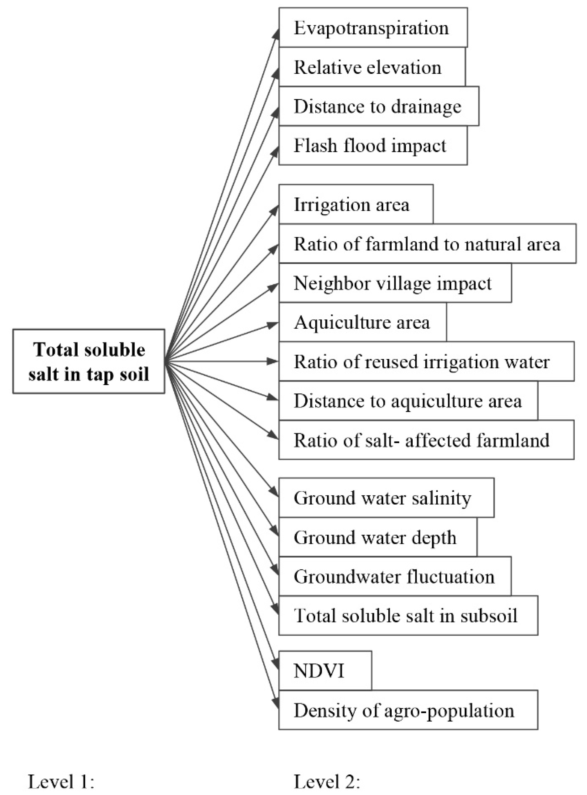
To solving the multi-criteria decision making problems as salinization, it is reasonable to use the AHP is a decision analysis method, which decomposing a complex problem into a hierarchical structure and estimates the relative importance of decision criteria (alternatives), a typical AHP has a three-level hierarchy, pairwise comparisons were using for setting priorities at each level [36]. In this study, a two-level hierarchy was developed (Figure 1)—the irrigation soil salinity risk is level 1 and the selected risk parameters are level 2. Employing AHP involves the following steps, for details refer to Reference [36]:
Step1: Structuring the issue in to a hierarchical model, this stage includes decomposing a complex issue into elements based on their characteristics and compose different level of model.
Step2: Making pair-wise comparison and obtaining a judgement matrix—at this stage, comparison of a pair of elements on each level by applying a nine-point scale. Due to some degree of subjectivity, the consistency of the pair-wise comparison matrix is checked, called consistency ratio (CR).
Step3: Aggregate the expert’s judgement, since each expert produce his or her own pair-wise comparison matrix, therefore, it is necessary to aggregate them into a group comparison by using weighted mean of comparisons is expressed as below in Equation (3):
where, the kth expert’s pair-wise comparison value is presented by , the number of expert is n and the kth expert’s weight is wk. In this work, all experts were assumed that they have equal expertise in their judgements. Then the final weight of all seventeen elements were obtained.
2.3.2. Objective Weight Assignment
In the objective weight assignment, the weights of relative importance of the parameters were calculated based on the curtain statistical method [33,48], that gives invaluable information about the data distribution. In this study, the maximizing deviation method (MDM) is selected to calculate the weights for parameters, because of the best reliability than method of standard deviation between classes, criteria importance through inter-criteria correlation and entropy method. Detailed information about this method can be found here [49,50]. The attribute weight W is equivalent to solving Equation (4), where Z is attribute matrix of data set to variable set.
2.3.3. Comprehensive Weight Assignment
The method of subjective assignment has randomness, while the objective method cannot reflect the importance of the index itself relative to the evaluation results [38]. Therefore, this study combines these two kinds of weights to get the comprehensive weights of each variable, attempt to makes a good use of measured data and to avoid the artificial effects on assessment, provide the decision maker with more accurate options to depend on.
The subjective and objective combination weighting were calculated by following methods (Equation (5)) [51]:
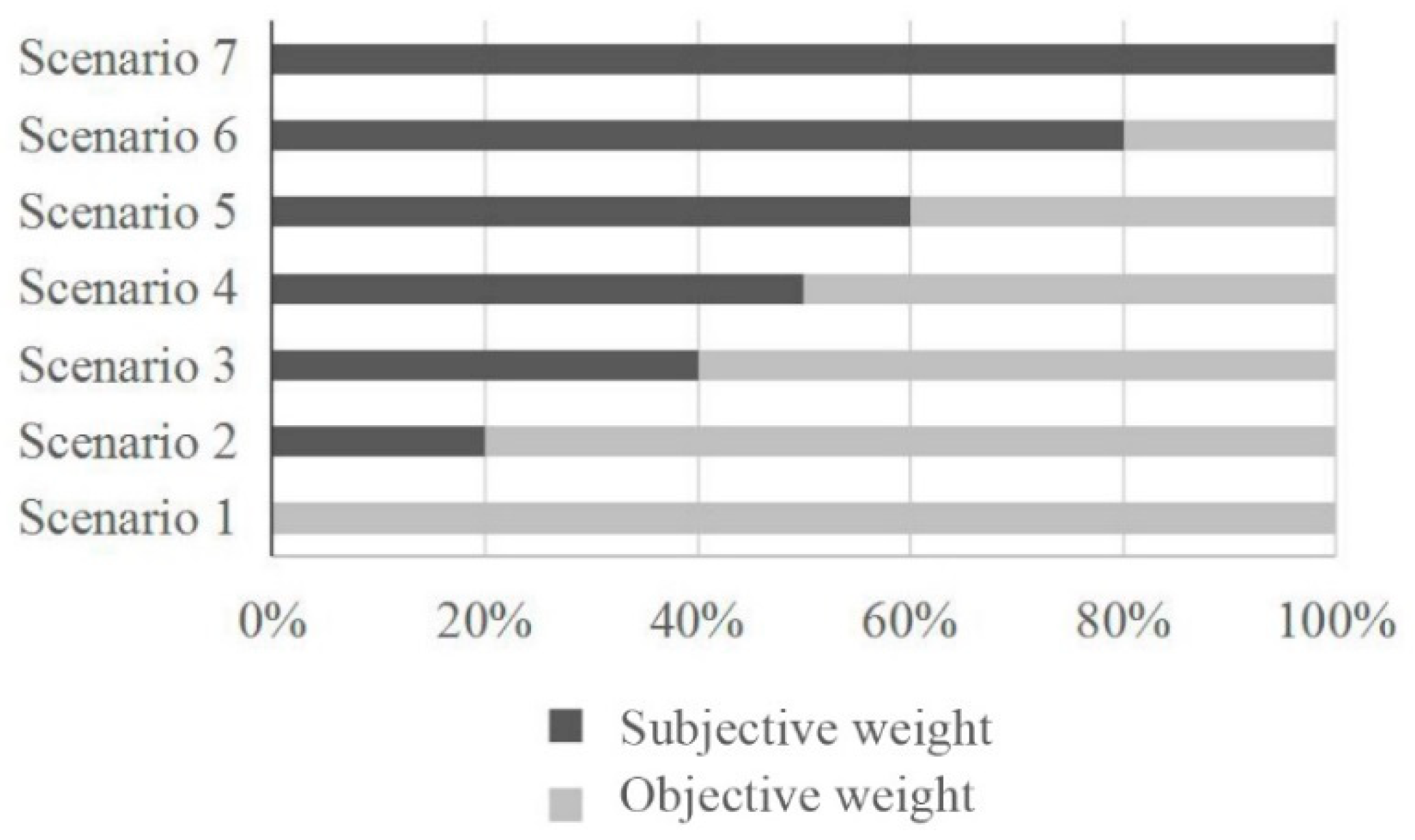
where, Wji is the integrated weight of jth variable and Ws and Wo are the weightages given to the objective and subjective weights respectively in different scenarios and the values of Ws and Wo are between 0 and 1. It indicates how much importance to assign to the objective and subjective weights of the jth variable. Under the different scenario, the few salinity risk maps were resulted, so to identify the most accurate salinity risk map, the scenario validation is necessary.
3. A Case Study on Keriya Oasis
3.1. Material and Methods
3.1.1. Study Area
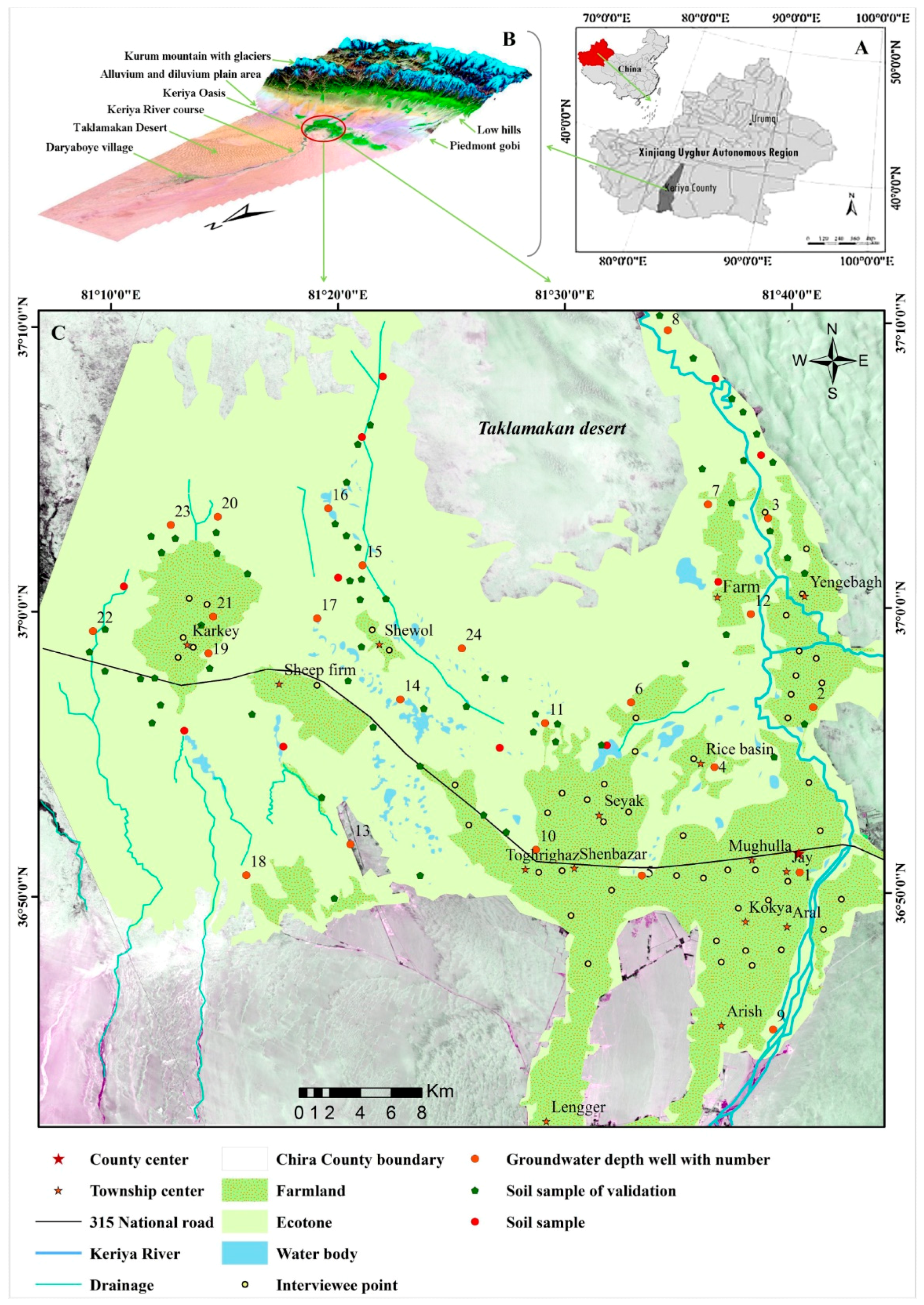
The Keriya Oasis is a County of the Xinjiang Uyghur Autonomous Regions. The Oasis is located on the alluvium and diluvium plain area between the southern margin of Taklimakan desert and the northern slope of Kurum (Kunlun in Chinese pinyin) mountain (Figure 2). The Oasis is surrounded by wide ecotone, which referring to the areas that located belt between neighboring deserts and an oasis in arid regions (Figure 2C). The ecotone are interactive zones between the natural ecosystem and irrigation activities [52]. The Oasis is characterized by dry warm climate (11.7 °C annually), scarce precipitation (45 mm annually), intensive potential evaporation (2500 mm annually), loose soil, highly mineralized underground water, high salt concentrations, lack of soil fertility and relatively flat topography [23]. The basin consists of five major landforms which include, in ascending order from north to south, the high mountains, low hills, piedmont gobi, alluvium and diluvium plain area and a large desert (Figure 1B). The agriculture providing most of the income and employment for population approximately about 250,000, the main crops are wheat, maize, cotton, rice and grapes. Agricultural activities mainly depends on water resources of the Keriya River, which is supplied by 430 glaciers in the Mountains [53]. The river disappears in the Derya Boyi village after approximately 700 km of flow [2]. Increasing socio-economic development have driven the expansion of the Oasis deep into the marginal ecotone zone [54,55]. Irrational using of water and land resources has caused water shortages in some areas, meanwhile caused soil salinization in others in the Oasis.
3.1.2. Risk Parameters of Composite Risk Index for Irrigation Salinity
The seventeen risk parameters were selected from the socio-environmental dimension but the economical dimension was ignored, since there is no noticeable difference in economic conditions among neighbor villages in the Oasis, which was proven by local official statistical data. The seventeen risk parameter include sixteen impacted factors and one impact receptor; among them, the eleven parameters as A0, A1, A2, A7, A8, A11, A12, A13, A14, A15 and A16 were identified from previous study; the five parameters as A3, A4, A6, A9 and A10 were suggested by stake holders; and one parameter as A5 was determined by expert suggestion (Table 1).
3.1.3. Data Collection and Analysis
Traditional Knowledge
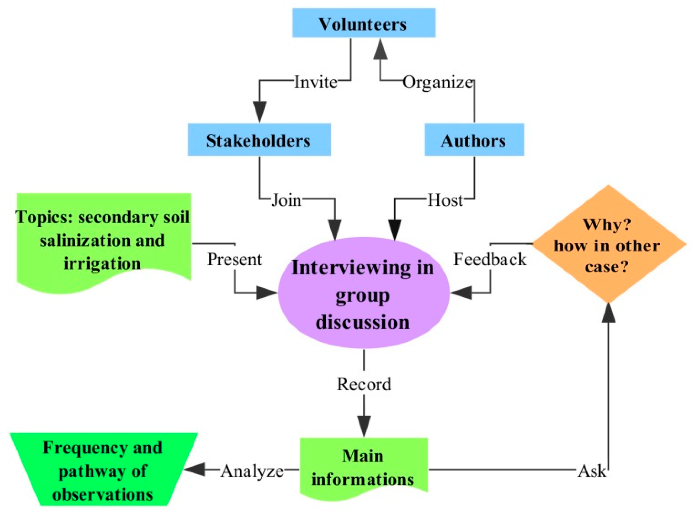
Stakeholder suggestions can provide supplemental sources of knowledge. To achieve traditional knowledge, semi-structured questionnaires were used during group consultations. This technique not only extracts useful potential information but also corrects and verifies information discussed in the group [58]. To achieve the effective interviewing, the volunteer assistants (students whom local to the Keriya Oasis) were organized. The 354 male farmers (according to traditional values, farm work is done by men) were visited randomly during February 201. A total of 51 interviews were held, with 6–9 attendees for each (Figure 1C). Farmer ages were <40 years (21%), 40–60 years (56%) and >60 years (23%), all people had a primary education at least. The main question discussed was, “what is the Oasis’s soil salinization trend during 1950–2010s?” Based on the stakeholder’s opinion, feedback questions were asked about the trend, locations and reasons for the trend of each observation—for instance, asking them if they think the soil salinization in the oasis is expanding and if the response is yes, to then ask them where. And what reasons caused this trend. The Figure 3 illustrates the steps and routines of collecting stakeholder’s opinion.
Soil and Groundwater Data
Ten field surveys were carried out between 2011 and 2015, mainly during dry seasons (from May to October). Thirty-five field investigation sites were selected for soil sampling (Figure 1C), which covers a range of land covers and soil characteristics. Each time the 50 g soil samples were collected in aluminum sampling boxes of 35 soil–sampling profiles (0.0–0.1 m, 0.1–0.2 m, 0.2–0.4 m, 0.4–0.6 m, 0.6–0.8 m and 0.8–1.0 m depth); electrical conductivity (EC) was measured by a field instrument (Hydra probe II, ds/m) for verification with laboratory measurements. In the laboratory, the total soluble salt content (in g/kg) was calculated by using a regression equation established between EC and total soluble salt [1]. The data from the first field survey were used for this study, others were referenced with this. In addition, in October 2015, another sixty soil samples were taken randomly from the topsoil (0–20 cm) (Figure 1C); they were used for validation and accuracy assessment of the scenario results. The 24 groundwater observation wells were used to collect the groundwater salinity (mS/cm) and depth (m), each well was equipped with HOBO U24-002-C and HOBO Barometric Sensor, all of them drilled in April 2012, sampling range of about 4–8 km. The datasets for the period of May 2012 to May 2013 are compiled in this study. The soil sampling sites and groundwater observation wells were positioned with a handheld GPS (Garmin, eTrex H, Olathe, KS, USA) [2] (Figure 1C).
3.2. Spatial Distribution of Risk Parameters
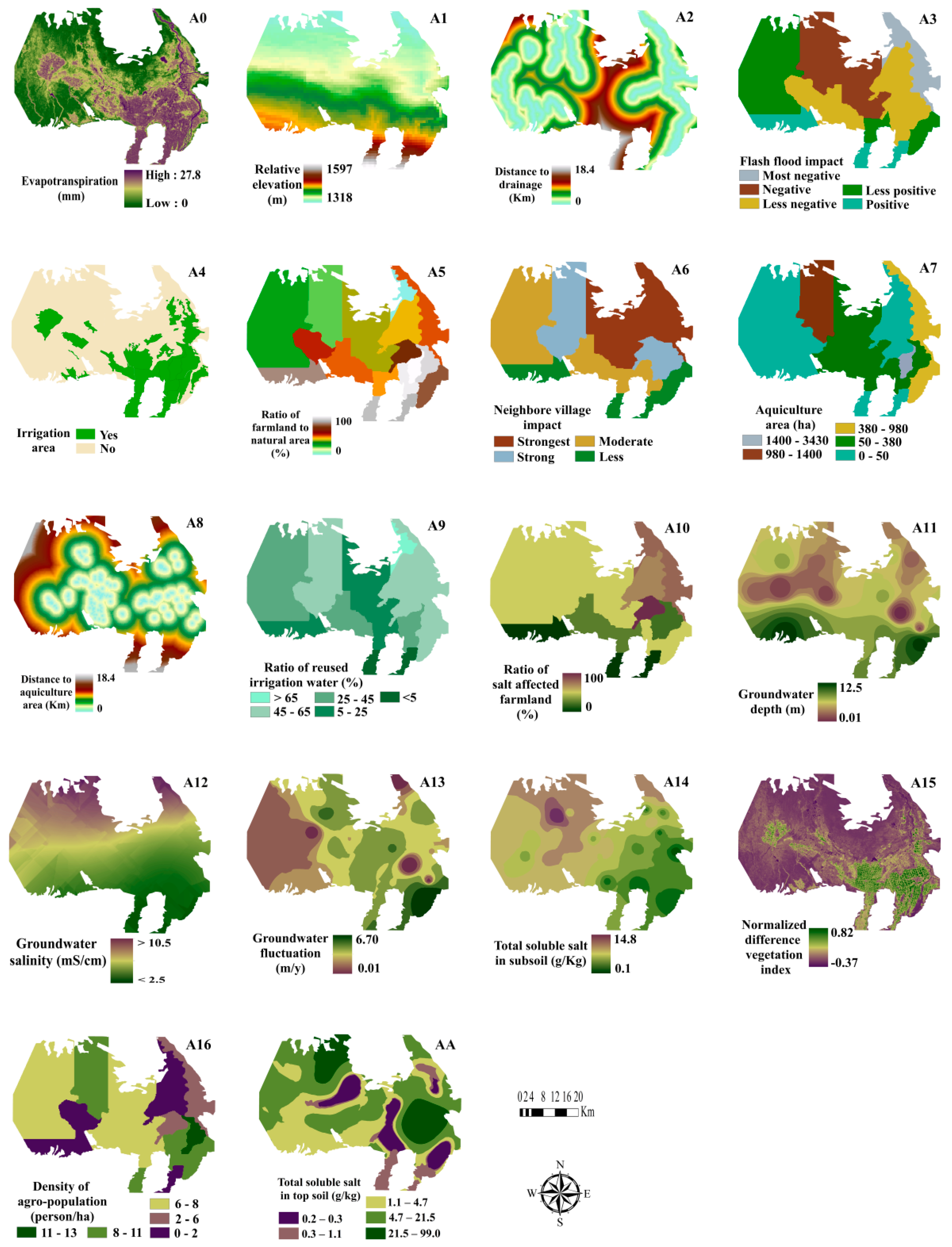
In this research, we used Arc GIS 10.1 and ENVI 5.1 for producing visualized spatial distribution of salinity risk parameters (in Figure 4); the data sources are presented in Table 1. In detail, the granger method was employed for estimating A0, which applied a conventional evapotranspiration model, estimates daily actual evapotranspiration, further details and steps referring to this can be found in Reference [56]. The A1 is built from freely available online data in 3D analysis tool (Table 1). The A0, A1 and A15 were visualized in the raster calculation tool. For example, the A2 and A8 were visualized by following steps: Spatial analyst → distance → straight line. The A3, A4, A6 were qualified and A5, A7, A9, A10, A16 were quantified thematic maps. Regarding the qualified maps, the literature was translated into numbers (in A6, strongest, strong, moderate and less were represented by 4, 3, 2 and 1, respectively). The kriging method (Spherical model) for spatial interpolation was performed with the geostatistical Wizard to calculate the Oasis-wide distribution of A11, A12, A13, A14 and AA [2], it estimates the value of parameters at unsampled locations based on the weighted average of the samples around it. In here, Gaussian distributions test was conducted for data sets in SPSS 20 before being used in the Spherical model, results that each Sig. of A11, A12, A13, A14 and AA were all less than 0.55, statistically acceptable. Then model predictions accuracy was estimated by the root-mean-square error (RMSE) which should be as small as possible and the standardized mean error (ME) which should be close to zero, in this work, the each RMSE and ME of A11, A12, A13, A14 and AA were all less than 6.0 and −0.25, respectively.
3.3. Calculation of Parameter and Weights
3.3.1. Weights of AHP
The pairwise comparison matrix was established by interviewing fourteen relevant specialists in the topic field and used for calculation of the weights of seventeen parameters (Table 2), each of the hierarchical level be weighted in terms of an overall criterion in a direct comparison between pairs of criteria. 1 is the equal significance; 2 is somewhat more significant; 5 is considerable significant; 7 is extremely more significant; 9 is absolutely dominant significance; and 2, 4, 6, 8 were intermediate values [60]. In this study, the issue decomposed into seventeen elements, so sub-points were inserted into the nine-point scale (Table 2).
3.3.2. Parameter Calculation
When spatial distribution of each parameter was completed in Arc GIS 10.1 [61], the risk receptor (total soluble salt of 35 sampling point) were added into the each parameter in Arc GIS10.1, then used the extraction tool, calculate the A0, A1, A11, A12, A13, A14 and A15; used the distance measuring tool to calculate the A2 and A8; and the A3, A4, A5, A6, A7, A9, A10 and A16 were the thematic maps in village level, means all point placed in a village has equal futures but during the field observation, we witnessed that a village also has diverse features of eco-environment, in order to match to real condition, the 35 sample points were assigned the values at by following principle: first step was divided the 35 sample point in to curtain group by value of thematic map, assign them equal value, then according to expert suggestions whose familiar well to the Oasis and attended the field investigation, the minor adjustment to sampling point of each group were conducted subjectively.
3.3.3. Calculation of MDM, rij and CRI
The MDM, rij and CRI were calculated by Equations (1)–(3) from various sources of data, those data sets were in different units and in different feature. So for this reason, normalization is crucial for rational statistics and comparison. There are many normalization methods, in this work, we normalized the data sets by using the Equations (5) and (6) as following [61]:
According to actual correlation of each parameter with top soil salinity, the parameters were grouped in to two groups, one is negatively related to top soil salinity (e.g., A1, A2, A4, A5, A8, A11, A13, A15 and A16); another is positively related to it (e.g., A0, A3, A6, A7, A9, A10, A12 and A14). The Equation (5) was used in first group, since negative impacts became larger, then the salinity risk is lower; and The Equation (4) was used in second group, since positive impact became larger, then the salinity risk is lower.
3.3.4. Spatial Distribution of CRI
When the values of CRI were calculated by the methods of the above section, then a spatial visualization of CRI was performed in Arc GIS10.1 according to the following steps: the first step was to reclassify the seventeen parameters presented in Section 3.2; the second step was to calculate the CRI of each scenario by using Equation (4); the third step was to combine the reclassified spatial parameters and calculate the CRI by using the raster calculator in a spatial analyst tool with Equation (7).
where Goal represents the spatial distribution of CRI of irrigation salinity, An represents the spatial distribution of every parameter and CRIAn represents the CRI value of the An parameter.
Goal = A1 × CRIA1 + A2 × CRIA2 + … + An × CRIAn n = 0, 1, 2, …, 16
3.4. Scenario Validation
The definition of risk is “possibility of loss or injury” that inferred the risk has prediction means of result. In this study, for validating the most accurate salinity risk map from seven maps of scenarios, additional 60 surface soil samples (0~20 cm) were collected in October 2015 (Figure 1C), four years later than research data (sampled in May 2011), this time gap produces a rational time interval of predicting the trend of soil salinity risk. The grey relational coefficients (rij) in Equation (2) were used to analyze the closeness between the CRI value and measured salt content and the higher rij value means higher accuracy.
4. Results
4.1. Composite Risk Index Values MDM, rij and CRI
The values for CRI are shown in Table 3. The evapotranspiration (A0), ground water depth (A11), ground water salinity (A12) and total soluble salt in subsoil (A14) have the greatest weight in calculation by AHP. Whilst aquiculture area (A7), ratio of reused irrigation water (A9) and ground water salinity (A12) have the greatest weight in calculation by MDM. This differences between AHP and MDM may be caused by subjectivity and objectivity of weight assignment. In addition, the greatest rij are found in total soluble salt in subsoil (A14), evapotranspiration (A0), irrigation area (A4), aquiculture area (A7), ratio of salt-affected farmland (A10), ground water salinity (A12), subsoil salinity (A14), those signifies the irrigation-induced salinity in the Oasis.
4.2. Scenario Validation
The CRI value was calculated using comprehensive assignment from the objective and subjective weight (Figure 5). Notably, in scenario 1, the CRI value was calculated using objective weights, and in scenario 7, it was calculated using subjective weights. The validation result indicated that (Figure 6), the map of scenario 5 reflected a higher rij than others, which means that it has higher closeness to reality of salinity risk distribution.
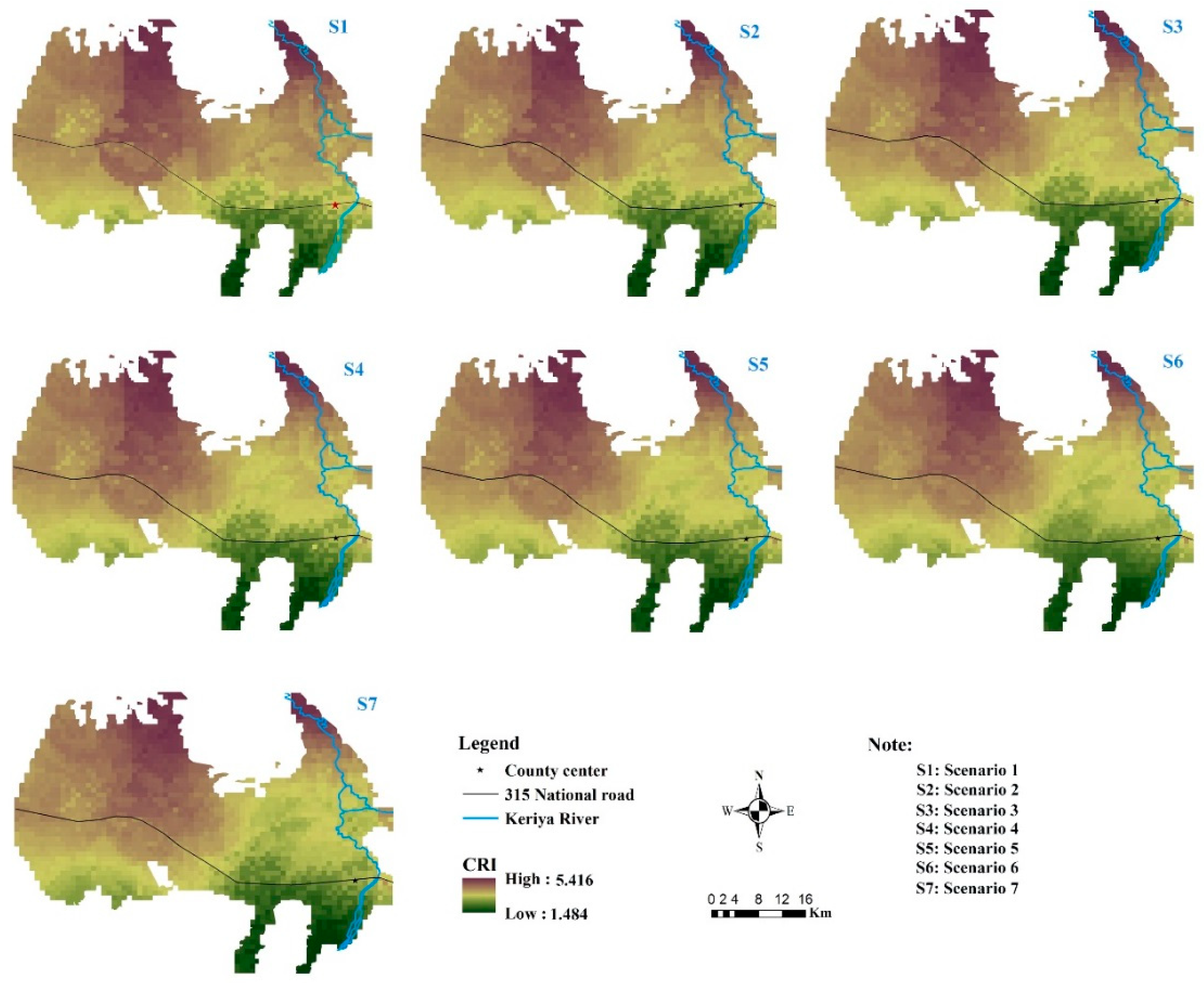
Figure 7 displays the spatial distribution of the CRI values of seven scenarios calculated using the comprehensive weights methodology for the Keriya Oasis. When looking at the spatial distributions, it is evident that salinity risk of the seven scenarios has regional characteristics of distribution; the general trend is similar among them. However, there is an obvious difference in salinity intensity between them. This explains that the salinity risk distribution maps are sensitive to changes of variable weights; simultaneously, it requires validation of these maps for determining the most accurate map.
This map of scenario 5 was most accurate one, characterized by clear grade in distribution of CRI density, soil salinity is very sensitive to earth surface, it is proved even one meter differences in surface can cause huge differences in salt content [62]. In addition, during field-work it was found that the Keriya Oasis ground surface is uneven. Thus, we are confident to say that the map of scenario 5 is the best map. Besides, this result proved that the combination of 40% of objective weight and 60% of subjective weight is the best weight assignment approach to salinity risk assessment in the Keriya Oasis.
4.3. Spatial Distribution of Salinity Risk Index
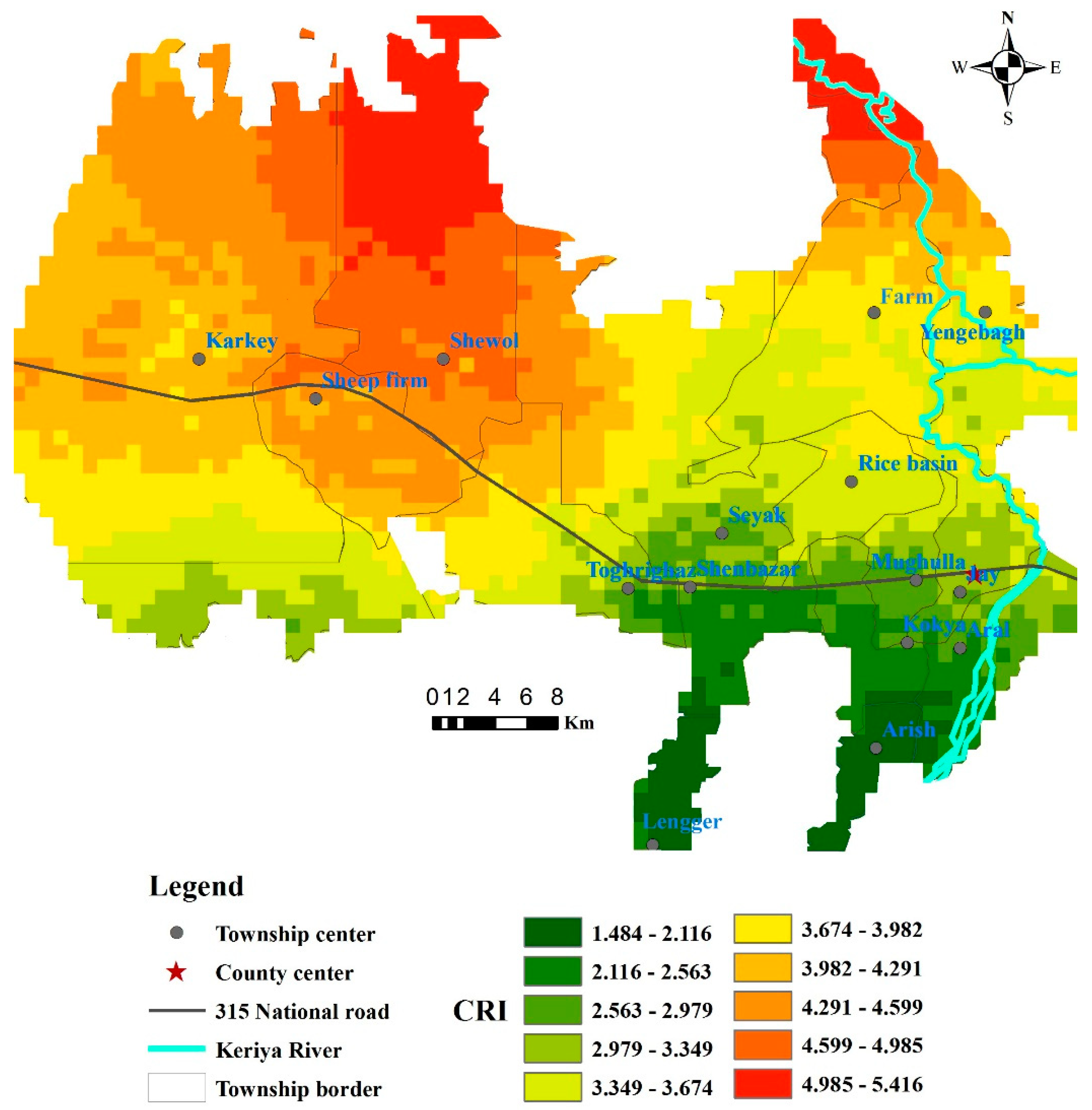
The spatial distribution of the CRI values for the Keriya Oasis was displayed in Figure 8. The values of CRI ranged between 1.484 and 5.416. To achieve effective analysis, the continuous CRI values were classified into ten classes. The distribution map of CRI indicated that irrigation salinity risk in the Keriya Oasis has regional features. The northwestern region has highest salinity risk, particularly, northern part of Shewol and Yeghebagh village (CRI is 4.985–5.416). The southern part of Shewol and the northeast part of Karkey and some areas of Yengebagh have a high risk of salinity (CRI is 4.599–4.985). And northern part of Karkey and sheep firm has moderate salinity risk (CRI is 4.291–4.599). Yet other regions (CRI of 4.291–3.349) has less salinity risk, these regions were characterized by the shallowest and constant groundwater table, low and flat enclosed terrain, large aquiculture area, lowest NDVI values, highest total soluble salt in subsoil and groundwater (refer to Figure 3). The southern region of the Oasis has lowest salinity risk with CRI of 3.349–1.484, where has higher relative elevation, deep high groundwater table, low soluble salt in subsoil and groundwater, all of them is former cultivated land (referring to Figure 3). Namely, the Lenger, Arish, Kokya, Aral, Shenbazar, Mughulla, Jay and southern part of Toghrighaz were more favorable to natural conditions for irrigation agriculture by low salinity risk.
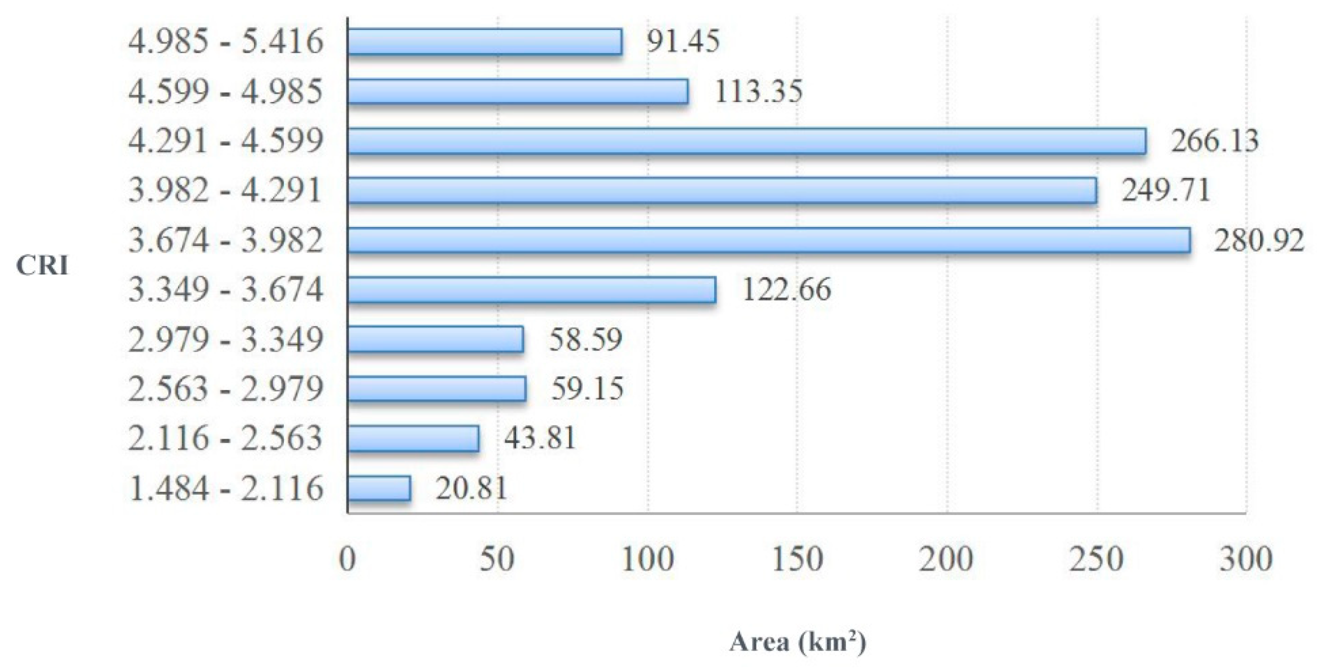
Summing up, salinity risk of Keriya Oasis characterized by less salinized and severe salinized areas occupy minor areas respectively and moderate salinized area form majority of whole Oasis (Figure 9).
5. Discussion
The Keriya Oasis’s ecosystem is very fragile and salinization and desertification threatens Oasis constantly, it has experienced frequent land reclamation and land abandonment due to soil salinity events [1,2,22]. The aim of our study was to show the spatial distribution of salinity hazard, the methodology combined use the maximizing deviation method and the analytical hierarchy process during integration of traditional and scientific knowledge by using the PSR framework and the grey relational analysis. The idea of this study is the first attempt to combined use subjective and objective weight assignment in the topic [34,35,63,64]. With diverse parameters by observing within broader view of study, this results even close to the actual situation of salinity risk.
It is proved again that the PSR framework not only has a systematic way to select parameters for irrigation salinity risk assessment and mapping but also helps to describe the threating problem for regional sustainability across the full spectrum rather a few individual parameters that only explains a portion of the issue (Table 4) [14,17,19,21,65]. However, using the PSR framework for risk index development has some limitations as well, over simplification may fail to indicate how the mechanism between parameters in real multi-level problems [66]. For instance, an irrigation area can be considered as a pressure if it is perceived to increase the ground water table, or a state of salinity hazard when it is thought to reflect the land's favorability for agriculture but these limitations can be solved by reviewing relevant research results.
The employed methodology is that it combines the objective weight assignment (MDM) and subjective weight assignment (AHP) to derive a weight calculative method for irrigation salinity risk assessment and mapping. in the AHP, the relative importance of risk parameters perceived by expert preference subjectively, lack of randomness and objectivity [8] and in the MDM, the relative importance of risk parameters calculated by curtain statistical approach objectively, lack of expert knowledge and experience about the local salinity problem [49]. Therefore, our proposed method combines the knowledge-based AHP and data-driven MDM, attempt to complement one another in approaches.
The Keriya Oasis’s salinity risk map (Figure 6) developed in this study is more reasonable than less accurate data derived remote-sensing images (Table 4) but this result can be improved if the data were collected in further high resolution, for example, Karkey village is so large in area, this may produce some bias in risk mapping when using the anthropogenic data. Although the salinity risk map of Keriya Oasis (Figure 6) was determined from seven maps (Figure 5) by validation approach and by actual measured data, result shows that the combination of objective and subjective weight assignment is the best weight assignment approach. However, there is some imparity between the risk data and the measured data, it is worth considering further validation when the new approaches were available.
The salinity risk map provides basic data for ecological designing and managing the Keriya Oasis. It is evident that different level of salinity risk must be applied different salinity control measures. Our results demonstrated that the northern part of the Shewol and Yeghebagh village have very high levels of salinity (Figure 6) which might be caused by a combined influence of flat and low enclosed terrain, shallow groundwater table, high total soluble salt in subsoil and groundwater. From above, we can conclude that the Oasis had inherent salinity problem, which may pose very big challenge for us that it is economically unfeasible to restore the salinized lands in this region. In comparison, the region with high salinity risk caused by excessive water logging and large aquiculture area (Figure 6), the main approach is to decrease the water body area by reducing water inlet to the area and increase water withdrawing by pumping or build drainage channel. In addition, the areas (Figure 6) were mainly subjected to a higher groundwater table, reused irrigation water (poor in quality) and poor drainage. The best approach may be to withdraw water by pumping, building drainage and plant salt tolerant plants. Besides, another approach to controlling salinity in this Oasis may be to reduce the use of irrigation water quantity, so deep percolation was decreased to maintain groundwater table depth whole oasis scale. For example, in the rice basin, rice cultivation is the dominant land use, it is suggested that alter the basin to dry land crops. In addition to this, according to stakeholders, irrigation activities in the southern part of Oasis can increase salinity risk to the northern part by water seepage, therefore, it is necessary to implement ecological designing plan about irrigation and drainage [52].
6. Conclusions
Our research assessed and mapped the spatial distribution of irrigation salinity risk in the Keriya Oasis by using seventeen relative parameters from traditional and scientific knowledge along with interdisciplinary and comprehensive methodology. The northern part of the Shewol and Yeghebagh village has a very high salinity risk; this might be caused by a combination of flat and low enclosed terrain, high total soluble salt in subsoil and groundwater and a shallow groundwater level. It is suggested that there is no economically feasible solution to this problem. In addition, a few other regions in the northern part of the Oasis have a relatively higher salinity risk. It is possible to restore the salinized area by artificial measures such as building drainage and decreasing the water logging. Therefore, the outcome is basic data for regional salinity management in the Keriya Oasis. In addition, the southern part of the Oasis has a relative low salinity risk and is suitable for irrigation agriculture.
Author Contributions
J.S. designed and wrote this paper, performed the experiments and fieldwork; G.-H.L. conceived this study; A.A. performed the experiments and fieldwork; Q.-D.S. was responsible expert’s knowledge; A.A. performed the fieldwork and ET calculation; A.T. performed the fieldwork.
Funding
This research was funded by [National Natural Science Foundation of China] grant number [31560131] and [National Natural Science Foundations of China] grant number [41671348].
Acknowledgments
We extend our gratitude to the field work assistants, hospitable interviewees. We also acknowledge the anonymous reviewers for their valuable comments.
Conflicts of Interest
The authors declare no conflict of interest.
References
- Nurmemet, I.; Ghulam, A.; Tiyip, T.; Elkadiri, R.; Ding, J.L.; Maimaitiyiming, M.; Abliz, A.; Sawut, M.; Zhang, F.; Abliz, A.; et al. Monitoring soil salinization in Keriya River Basin, Northwestern China using passive reflective and active microwave remote sensing data. Remote Sens. 2015, 7, 8803–8829. [Google Scholar] [CrossRef]
- Abliz, A.; Tiyip, T.; Ghulam, A.; Halik, Ü.; Ding, J.L.; Sawut, M.; Zhang, F.; Nurmemet, I.; Abliz, A. Effects of shallow groundwater table and salinity on soil salt dynamics in the Keriya Oasis, Northwestern China. Environ. Earth Sci. 2016, 75, 260. [Google Scholar] [CrossRef]
- Peck, A.J.; Hatton, T. Salinity and the discharge of salts from catchments in Australia. J. Hydrol. 2003, 272, 191–202. [Google Scholar] [CrossRef]
- Herrero, J.; Pérez-Coveta, O. Soil salinity changes over 24 years in a Mediterranean irrigated district. Geoderma 2005, 125, 287–308. [Google Scholar] [CrossRef] [Green Version]
- Corwin, D.L.; Rhoades, J.D.; Šimůnek, J. Leaching requirement for soil salinity control: Steady-state versus transient models. Agric. Water Manag. 2007, 90, 165–180. [Google Scholar] [CrossRef]
- Pannell, D.J.; Ewing, M.A. Managing secondary dryland salinity: Options and challenges. Agric. Water Manag. 2006, 80, 41–56. [Google Scholar] [CrossRef]
- Wiebe, B.H.; Eilers, R.G.; Eilers, W.D.; Brierley, J.A. Application of a risk indicator for assessing trends in dryland salinization risk on the Canadian Prairies. Can. J. Soil Sci. 2007, 87, 213–224. [Google Scholar] [CrossRef] [Green Version]
- Zhou, D.; Lin, Z.; Liu, L.; Zimmermann, D. Assessing secondary soil salinization risk based on the PSR sustainability framework. J. Environ. Manag. 2013, 128, 642–654. [Google Scholar] [CrossRef] [PubMed]
- Aragüés, R.; Urdanoz, V.; Çetin, M.; Kirda, C.; Daghari, H.; Ltifi, W.; Lahlou, M.; Douaik, A. Soil salinity related to physical soil characteristics and irrigation management in four Mediterranean irrigation districts. Agric. Water Manag. 2011, 98, 959–966. [Google Scholar] [CrossRef] [Green Version]
- Hamzeh, S.; Naseri, A.A.; AlaviPanah, S.K.; Mojaradi, B.; Bartholomeus, H.M.; Clevers, J.G.P.W.; Behzad, M. Estimating salinity stress in sugarcane fields with spaceborne hyperspectral: Vegetation indices. Int. J. Appl. Earth Obs. Geoinf. 2012, 21, 282–290. [Google Scholar] [CrossRef]
- Wang, Q.; Li, P.; Chen, X. Modeling salinity effects on soil reflectance under various moisture conditions and its inverse application: A laboratory experiment. Geoderma 2012, 170, 103–111. [Google Scholar] [CrossRef]
- Metternicht, G.I.; Zinck, J.A. Remote sensing of soil salinity: Potentials and constraints. Remote Sens. Environ. 2003, 85, 1–20. [Google Scholar] [CrossRef]
- Akramkhanov, A.; Martius, C.; Park, S.J.; Hendrickx, J.M.H. Environmental factors of spatial distribution of soil salinity on flat irrigated terrain. Geoderma 2011, 163, 55–62. [Google Scholar] [CrossRef]
- Akramkhanov, A.; Brus, D.J.; Walvoort, D.J.J. Geostatistical monitoring of soil salinity in Uzbekistan by repeated EMI surveys. Geoderma 2014, 213, 600–607. [Google Scholar] [CrossRef]
- Huang, J.; Prochazka, M.J.; Triantafilis, J. Irrigation salinity hazard assessment and risk mapping in the lower Macintyre Valley, Australia. Sci. Total Environ. 2016, 551–552, 460–473. [Google Scholar] [CrossRef] [PubMed]
- Niemeijer, D.; de Groot, R.S. A conceptual framework for selecting environmental indicator sets. Ecol. Indic. 2008, 8, 14–25. [Google Scholar] [CrossRef]
- Grundy, M.J.; Silburn, D.M.; Chamberlain, T. A risk framework for preventing salinity. Environ. Hazards 2007, 7, 97–105. [Google Scholar] [CrossRef]
- Yao, R.; Yang, J. Quantitative evaluation of soil salinity and its spatial distribution using electromagnetic induction method. Agric. Water Manag. 2010, 97, 1961–1970. [Google Scholar] [CrossRef]
- Zhou, D.; Lin, Z.; Liu, L.; State, N.D.; Dakota, N. Developing a Composite Risk Index for Secondary Soil Salinization Based on the PSR Sustainability Framework. Ph.D. Thesis, International Environmental Modelling and Software Society (iEMSs), Manno, Switzerland, 2012. [Google Scholar]
- Lobell, D.B.; Lesch, S.M.; Corwin, D.L.; Ulmer, M.G.; Anderson, K.A.; Potts, D.J.; Doolittle, J.A.; Matos, M.R.; Baltes, M.J. Regional-scale assessment of soil salinity in the Red River Valley using multi-year MODIS EVI and NDVI. J. Environ. Qual. 2010, 39, 35–41. [Google Scholar] [CrossRef] [PubMed]
- Huang, H.F.; Kuo, J.; Lo, S.L. Review of PSR framework and development of a DPSIR model to assess greenhouse effect in Taiwan. Environ. Monit. Assess. 2011, 177, 623–635. [Google Scholar] [CrossRef] [PubMed]
- Eziz, M.; Yimit, H.; Mohammad, A.; Huang, Z. Oasis land-use change and its effects on the oasis eco-environment in Keriya Oasis, China. Int. J. Sustain. Dev. World Ecol. 2010, 17, 244–252. [Google Scholar] [CrossRef]
- Gong, L.; Ran, Q.; He, G.; Tiyip, T. A soil quality assessment under different land use types in Keriya river basin, Southern Xinjiang, China. Soil Tillage Res. 2015, 146, 223–229. [Google Scholar] [CrossRef]
- Zhou, D.; Lin, Z.; Liu, L. Regional land salinization assessment and simulation through cellular automaton-Markov modeling and spatial pattern analysis. Sci. Total Environ. 2012, 439, 260–274. [Google Scholar] [CrossRef] [PubMed]
- Huffman, E.; Eilers, R.G.; Padbury, G.; Wall, G.; MacDonald, K.B. Canadian agri-environmental indicators related to land quality: Integrating census and biophysical data to estimate soil cover, wind erosion and soil salinity. Agric. Ecosyst. Environ. 2000, 81, 113–123. [Google Scholar] [CrossRef]
- Kairis, O.; Kosmas, C.; Karavitis, C.; Ritsema, C.; Salvati, L.; Acikalin, S.; Alcalá, M.; Alfama, P.; Atlhopheng, J.; Barrera, J.; et al. Evaluation and selection of indicators for land degradation and desertification monitoring: Types of degradation, causes, and implications for management. Environ. Manag. 2013, 54, 971–982. [Google Scholar] [CrossRef] [PubMed]
- Kosmas, C.; Kairis, O.; Karavitis, C.; Acikalin, S.; Alcalá, M.; Alfama, P.; Atlhopheng, J.; Barrera, J.; Fernandez, F.; Gokceoglu, C.; et al. An exploratory analysis of land abandonment drivers in areas prone to desertification. Catena 2014, 128, 252–261. [Google Scholar] [CrossRef]
- Zhang, T.-T.; Zeng, S.-L.; Gao, Y.; Ouyang, Z.-T.; Li, B.; Fang, C.-M.; Zhao, B. Assessing impact of land uses on land salinization in the Yellow River Delta, China using an integrated and spatial statistical model. Land Use Policy 2011, 28, 857–866. [Google Scholar] [CrossRef]
- Maxim, L.; Spangenberg, J.H.; O’Connor, M. An analysis of risks for biodiversity under the DPSIR framework. Ecol. Econ. 2009, 69, 12–23. [Google Scholar] [CrossRef]
- Böhringer, C.; Jochem, P.E.P. Measuring the immeasurable—A survey of sustainability indices. Ecol. Econ. 2007, 63, 1–8. [Google Scholar] [CrossRef]
- Kondyli, J. Measurement and evaluation of sustainable development: A composite indicator for the islands of the North Aegean region, Greece. Environ. Impact Assess. Rev. 2010, 30, 347–356. [Google Scholar] [CrossRef]
- Floridi, M.; Pagni, S.; Falorni, S.; Luzzati, T. An exercise in composite indicators construction: Assessing the sustainability of Italian regions. Ecol. Econ. 2011, 70, 1440–1447. [Google Scholar] [CrossRef]
- Shaker, R.R. A mega-index for the Americas and its underlying sustainable development correlations. Ecol. Indic. 2018, 89, 466–479. [Google Scholar] [CrossRef]
- Berkes, F.; Colding, J.; Folke, C. Rediscovery of traditional ecological knowledge as adaptive management. Ecol. Appl. 2010, 10, 1251–1262. [Google Scholar] [CrossRef]
- Ambrose, W.G.; Clough, L.M.; Johnson, J.C.; Greenacre, M.; Griffith, D.C.; Carroll, M.L.; Whiting, A. Interpreting environmental change in coastal Alaska using traditional and scientific ecological knowledge. Front. Mar. Sci. 2014, 1, 40. [Google Scholar] [CrossRef]
- Gupta, S.; Kumar, U. An analytical hierarchy process (AHP)—Guided decision model for underground mining method selection. Int. J. Min. Reclam. Environ. 2014, 26, 324–336. [Google Scholar] [CrossRef]
- Rao, R.V. Decision Making in Manufacturing Environment Using Graph Theory and Fuzzy Multiple Attribute Decision Making Methods; Springer-Verlag: London, UK, 2013; Volume 2, p. 4471. ISBN 978-1-4471-4375-8. [Google Scholar]
- Zhao, J.; Jin, J.; Zhu, J.; Xu, J.; Hang, Q.; Chen, Y.; Han, D. Water resources risk assessment model based on the subjective and objective combination weighting methods. Water Resour. Manag. 2016, 30, 3027–3042. [Google Scholar] [CrossRef]
- Spangenberg, J.H.; Douguet, J.M.; Settele, J.; Heong, K.L. Escaping the lock-in of continuous insecticide spraying in rice: Developing an integrated ecological and socio-political DPSIR analysis. Ecol. Model. 2015, 295, 188–195. [Google Scholar] [CrossRef]
- Dubey, A.K.; Yadava, V. Multi-objective optimization of Nd:YAG laser cutting of nickel-based superalloy sheet using orthogonal array with principal component analysis. Opt. Lasers Eng. 2008, 46, 124–132. [Google Scholar] [CrossRef]
- Singh, S. Optimization of machining characteristics in electric discharge machining of 6061Al/Al2O3p/20P composites by grey relational analysis. Int. J. Adv. Manuf. Technol. 2012, 63, 1191–1202. [Google Scholar] [CrossRef]
- Liu, S.; Yang, Y.; Forrest, J. Sequence Operators and Grey Data Mining. In Grey Data Analysis; Springer: Singapore, 2017; pp. 45–65. ISBN 978-981-10-1841-1. [Google Scholar]
- Deng, J.L. Control Problem of Grey Systems. Syst. Control Lett. 1982, 1, 288–294. [Google Scholar]
- Zeng, G.; Jiang, R.; Huang, G.; Xu, M.; Li, J. Optimization of wastewater treatment alternative selection by hierarchy grey relational analysis. J. Environ. Manag. 2007, 82, 250–259. [Google Scholar] [CrossRef] [PubMed]
- Pai, T.Y.; Hanaki, K.; Ho, H.H.; Hsieh, C.M. Using grey system theory to evaluate transportation effects on air quality trends in Japan. Transp. Res. Part D Transp. Environ. 2007, 12, 158–166. [Google Scholar] [CrossRef]
- Li, Z.-Z.; Li, W.-D.; Shi, H.-H.; Jia, X.-H. Gray model for ecological risk assessment and its application in salinization oasis agroecosystem. J. Desert Res. 2002, 22, 617–622. (In Chinese) [Google Scholar]
- Veisi, H.; Liaghati, H.; Alipour, A. Developing an ethics-based approach to indicators of sustainable agriculture using analytic hierarchy process (AHP). Ecol. Indic. 2016, 60, 644–654. [Google Scholar] [CrossRef]
- Wang, W.-D.; Guo, J.; Fang, L.-G.; Chang, X.-S. A subjective and objective integrated weighting method for landslides susceptibility mapping based on GIS. Environ. Earth Sci. 2012, 65, 1705–1714. [Google Scholar] [CrossRef]
- Wei, G.-W. Maximizing deviation method for multiple attribute decision making in intuitionistic fuzzy setting. Knowl.-Based Syst. 2008, 21, 833–836. [Google Scholar] [CrossRef]
- Zhang, H.; Mao, H. Comparison of four methods for deciding objective weights of features for classifying stored-grain insects based on extension theory. Trans. CSAE 2009, 25, 132–136. (In Chinese) [Google Scholar]
- Hashemi, H.; Mousavi, S.M.; Zavadskas, E.K.; Chalekaee, A.; Turskis, Z. A new group decision model based on Grey-Intuitionistic Fuzzy-ELECTRE and VIKOR for contractor assessment problem. Sustainbility 2018, 10, 1635. [Google Scholar] [CrossRef]
- Wang, Y.; Li, Y. Land exploitation resulting in soil salinization in a desert-oasis ecotone. Catena 2013, 100, 50–56. [Google Scholar] [CrossRef]
- Halik, W.; Tiyip, T.; Yimit, H.; He, L. Water resources utilization and eco-environmental changing research in Keriya Valley. Syst. Sci. Compr. Stud. Agric. 2006, 22, 283–287. (In Chinese) [Google Scholar]
- Jiang, Y.; Zhou, C.-H.; Cheng, W.-M. Streamflow trends and hydrological response to climatic change in Tarim headwater basin. J. Geogr. Sci. 2007, 17, 51–56. [Google Scholar] [CrossRef]
- Lu, F.; Xu, J.-H.; Chen, Y.-N.; Li, W.-H.; Zhang, L.-J. Annual runoff change and it’s response to climate change in the headwater area of the Yarkand River in the recent 50 years. Quat. Sci. 2010, 30, 152–158. (In Chinese) [Google Scholar] [CrossRef]
- Tsouni, A.; Kontoes, C.; Koutsoyiannis, D.; Elias, P.; Mamassis, N. Estimation of actual evapotranspiration by remote sensing: Application in Thessaly Plain, Greece. Sensors 2008, 8, 3586–3600. [Google Scholar] [CrossRef] [PubMed]
- Wei, Y.-L.; Wang, H.; Li, N. Keriya County Annals, 1st ed.; Xinjiang People’s Press: Urumqi, China, 2006; pp. 142–148, 162–164, 173–181, 300–313. ISBN 7-228-09260-0. (In Chinese) [Google Scholar]
- Huntington, H.P. Using Traditional Ecological Knowledge in Science: Methods and Applications. Ecol. Appl. 2000, 10, 1270–1274. [Google Scholar] [CrossRef]
- Seydehmet, J.; Lv, G.H.; Nurmemet, I.; Aishan, T.; Abliz, A.; Sawut, M.; Abliz, A.; Eziz, M. Model prediction of secondary soil salinization in the Keriya Oasis, Northwest China. Sustainability 2018, 10, 656. [Google Scholar] [CrossRef]
- Weck, M.; Klocke, F.; Schell, H.; Rüenauver, E. Evaluating alternative production cycles using the extended fuzzy AHP method. Eur. J. Oper. Res. 1997, 100, 351–366. [Google Scholar] [CrossRef]
- Forsythe, K.W.; Marvin, C.H.; Valancius, C.J.; Watt, J.P.; Aversa, J.M.; Swales, S.J.; Jakubek, D.J.; Shaker, R.R. Geovisualization of mercury contamination in Lake St. Clair Sediments. J. Mar. Sci. Eng. 2016, 4, 19. [Google Scholar] [CrossRef]
- Fan, Z.; Ma, Y.; Zhang, H.; Wang, R.; Zhao, Y.; Zhou, H. Research of eco-water table and rational depth of groundwater of Tarim River Drainage Basin. Arid Land Geogr. 2004, 27, 8–13. (In Chinese) [Google Scholar]
- Carter, B.T.G.; Nielsen, E.A. Exploring ecological changes in Cook Inlet beluga whale habitat though traditional and local ecological knowledge of contributing factors for population decline. Mar. Policy 2011, 35, 299–308. [Google Scholar] [CrossRef]
- Liedloff, A.C.; Woodward, E.L.; Harrington, G.A.; Jackson, S. Integrating indigenous ecological and scientific hydro-geological knowledge using a Bayesian Network in the context of water resource development. J. Hydrol. 2013, 499, 177–187. [Google Scholar] [CrossRef]
- Benyamini, Y.; Mirlas, V.; Marish, S.; Gottesman, M.; Fizik, E.; Agassi, M. A survey of soil salinity and groundwater level control systems in irrigated fields in the Jezre’el Valley, Israel. Agric. Water Manag. 2005, 76, 181–194. [Google Scholar] [CrossRef]
- Taylor, P.; Carr, E.R.; Wingard, P.M.; Yorty, S.C.; Thompson, M.C.; Jensen, N.K.; Roberson, J. Applying DPSIR to sustainable development. Int. J. Sustain. Dev. World Ecol. 2009, 14, 543–555. [Google Scholar] [CrossRef]
Figure 1.
Two-level structure of the AHP model for the Irrigation Salinity Risk Assessment and Mapping.
Figure 1.
Two-level structure of the AHP model for the Irrigation Salinity Risk Assessment and Mapping.

Figure 2.
Location map of the Keriya County of China and the Xinjiang Uyghur Autonomous Region (XUAR) (A); topographic map of Keriya River Basin (B); the map sampling points of the Keriya Oasis (C).
Figure 2.
Location map of the Keriya County of China and the Xinjiang Uyghur Autonomous Region (XUAR) (A); topographic map of Keriya River Basin (B); the map sampling points of the Keriya Oasis (C).

Figure 3.
Diagram of the consultation of stakeholders in order to investigate traditional knowledge and irrigation salinity knowledge, adapted from [59].
Figure 3.
Diagram of the consultation of stakeholders in order to investigate traditional knowledge and irrigation salinity knowledge, adapted from [59].

Figure 4.
Raster maps of the risk receptor and risk parameters in the Keriya Oasis.

Figure 5.
Integrated weight information.

Figure 6.
Scenario validation result.

Figure 7.
Spatial distribution of the composite risk index (CRI) in the Keriya Oasis. Note: When reclassifying the process of evapotranspiration, the lowest value was given for values greater than 15 mm; values of 15 mm and higher were placed in the irrigation area. Irrigation activity reduces salt salinity risk largely by the salt leaching function.

Figure 8.
Spatial distribution of the composite risk index (CRI) in the Keriya Oasis.

Figure 9.
Area statistics of CRI class.


Table 1.
Risk parameters within Pressure-State-Response (PSR) categories for irrigation salinity risk assessment and mapping in the Keriya Oasis.
Table 1.
Risk parameters within Pressure-State-Response (PSR) categories for irrigation salinity risk assessment and mapping in the Keriya Oasis.
| PSR | Parameters and Symbols | Explanations | Sources | Data Types |
|---|---|---|---|---|
| Pressures (Natural) | Evapotranspiration (A0) | The actual evapotranspiration (ΕΤ) was calculated based on Granger’s equation [56]; the common equation can be written as below: In the equations, ET is the daily actual evapotranspiration (mm day−1), ∆ is the gradient of vapor pressure curve (kP °C−1), Rn is the net radiation at the crop surface (ΜJ m−2 day−1), G is the soil heat flux density (ΜJ m−2 d−1), λ is the latent heat of vaporization (MJ kg−1), γ is the psychrometric coefficient (kP °C−1), Εα is the drying power of the air (mm d−1), g is the relative evaporation (–) | This study | Combination of mathematical model and Landsat-8 ETM+ * |
| Relative elevation (A1) | Height above sea level (m) | This study | GTOP30/DEM * | |
| Distance to drainage (A2) | Strait distance to River course (drainage is one of rivers’ dual functions due to seasonality) or natural drainage ditches (m) | This study | Landsat-8 ETM+ * | |
| Flash flood impact (A3) | Flash flooding (termed “Sel” in local) usually caused by heavy rain in the mountains, is always unexpected, fast-moving and destructive. Generally, it creates a natural powerful drainage at a relatively higher area by eroding the earth surface. It leads to a decrease of land slope by bringing mud sedimentation to the low areas | This study | Stakeholder’s opinion | |
| Pressures (Human) | Irrigation area (A4) | The cultivated area is irrigated frequently, reducing the salt by salt leaching and natural area | [22], This study | Stakeholder’s opinion, Landsat-8 ETM+ * |
| Ratio of farmland to natural area (A5) | The ratio of total farmland area of each village to its total area except desert area (%) | [57] | Statistical data, expert’s opinion | |
| Neighbor village impact (A6) | A village in the Oasis subject to the influences of its neighbor due to the catchment slopes from south to north. More farmland at higher elevation causes higher risk to its lower neighbor | This study | Stakeholder’s opinion | |
| Aquiculture area (A7) | Fish pond area of each village (ha) | [57] | Statistical data | |
| Distance to aquiculture area (A8) | Strait distance to the center of the fish pond or water reservoir (m) | This study | Landsat-8 ETM+ * | |
| Ratio of reused irrigation water (A9) | Irrigation time of reused water to not reused irrigation water (“Kara water/Aq water” in local term) (%), Kara water saltier than Aq water | This study | Stakeholder’s opinion | |
| States | Ratio of salt-affected farmland (A10) | Percentage of salt-affected farmland to fertile farmland (%). Salt-affected farmland was determined by field symptoms: The field is relatively wet but crops wither easily; and the field has a shallow groundwater table but requires regular irrigation. At maximum impact, fields would die entirely if they lost only one year of irrigation chance | This study | Stakeholder’s opinion |
| Ground water depth (A11) | Vertical distance from the soil surface to ground water table (m) | [2], This study | Field measured data | |
| Ground water salinity (A12) | Electric conductivity of groundwater (mS/cm) | [2], This study | Field measured data | |
| Groundwater fluctuation (A13) | Annual difference between the maximum value and minimum value (m/year) | [2], This study | Field measured data | |
| Total soluble salt in subsoil (A14) | Average total soluble salt content in the subsoil layer (0.4–0.6 m, 0.6–0.8 m, 0.8–1.0 m, depth) (g/Kg) | This study | Field and Lab. measured data | |
| Responses | NDVI (A15) | Normalized difference vegetation index, NDVI = (NIR − R)/(NIR + R), NIR is Near infrared band, R is red band | This study | Landsat-8 ETM+ * |
| Density of agro-population (A16) | Village labor number to total village arable area (person/per ha farmland) | [57] | Statistical data | |
| Total soluble salt in tap soil (AA) | Average total soluble salt content in the topsoil layer (0.0–0.1 m, 0.1–0.2 m, 0.2–0.4 m, depth) (g/Kg) | This study | Lab. measured data | |
Note: “*” were available at http://glovis.usgs.gov/; http://www.gscloud.cn/ resolution 30, cloud 0% for the selected study area, download date: 21 July 2015.
Table 2.
Pairwise comparison matrix and the normalized relative importance weight vector for the irrigation salinity risk assessment and mapping in the Keriya Oasis.
Table 2.
Pairwise comparison matrix and the normalized relative importance weight vector for the irrigation salinity risk assessment and mapping in the Keriya Oasis.
| Variable Symbols | A0 | A1 | A2 | A3 | A4 | A5 | A6 | A7 | A8 | A9 | A10 | A11 | A12 | A13 | A14 | A15 | A16 |
|---|---|---|---|---|---|---|---|---|---|---|---|---|---|---|---|---|---|
| A0 | 1.00 | ||||||||||||||||
| A1 | 2.00 | 1.00 | |||||||||||||||
| A2 | 0.50 | 0.43 | 1.00 | ||||||||||||||
| A3 | 0.14 | 0.20 | 0.67 | 1.00 | |||||||||||||
| A4 | 0.60 | 0.33 | 0.63 | 1.75 | 1.00 | ||||||||||||
| A5 | 0.17 | 0.67 | 0.80 | 1.13 | 0.33 | 1.00 | |||||||||||
| A6 | 0.20 | 0.25 | 0.40 | 1.25 | 0.20 | 0.40 | 1.00 | ||||||||||
| A7 | 0.50 | 1.50 | 1.33 | 1.17 | 1.14 | 1.13 | 1.33 | 1.00 | |||||||||
| A8 | 0.17 | 0.90 | 0.83 | 1.40 | 0.67 | 1.40 | 2.00 | 0.50 | 1.00 | ||||||||
| A9 | 0.13 | 0.67 | 0.67 | 0.80 | 0.14 | 0.33 | 4.00 | 0.33 | 1.33 | 1.00 | |||||||
| A10 | 0.17 | 0.33 | 1.10 | 0.67 | 0.17 | 0.25 | 4.00 | 0.33 | 0.60 | 0.25 | 1.00 | ||||||
| A11 | 3.50 | 3.00 | 5.50 | 6.50 | 1.50 | 4.50 | 4.00 | 1.50 | 3.00 | 6.00 | 7.00 | 1.00 | |||||
| A12 | 4.00 | 3.50 | 6.00 | 7.00 | 2.00 | 6.00 | 4.50 | 2.00 | 3.33 | 6.50 | 7.50 | 1.33 | 1.00 | ||||
| A13 | 2.33 | 2.00 | 4.00 | 5.00 | 1.00 | 4.00 | 2.50 | 1.00 | 2.00 | 4.00 | 5.00 | 0.78 | 0.43 | 1.00 | |||
| A14 | 3.00 | 2.67 | 5.00 | 6.00 | 1.13 | 4.33 | 3.33 | 1.25 | 2.33 | 5.00 | 6.00 | 0.88 | 0.60 | 0.80 | 1.00 | ||
| A15 | 0.13 | 0.75 | 0.50 | 2.00 | 0.89 | 0.88 | 3.00 | 0.20 | 0.33 | 1.00 | 0.67 | 0.13 | 0.14 | 0.17 | 0.14 | 1.00 | |
| A16 | 0.20 | 2.00 | 0.33 | 0.33 | 0.50 | 2.00 | 0.67 | 0.17 | 0.25 | 0.33 | 4.00 | 0.20 | 0.25 | 0.33 | 0.50 | 4.00 | 1.00 |
Notations: CR = 0.08395.
Table 3.
Weights of the analytic hierarchy process (AHP) and maximizing deviation method (MDM); values of grey relational coefficients (rij) and the composite risk index (CRI) for secondary salinity risk assessment and mapping in the Keriya Oasis.
Table 3.
Weights of the analytic hierarchy process (AHP) and maximizing deviation method (MDM); values of grey relational coefficients (rij) and the composite risk index (CRI) for secondary salinity risk assessment and mapping in the Keriya Oasis.
| Variable Symbols | AHP Weights | MDM Weights | rij | CRI Value | ||||||
|---|---|---|---|---|---|---|---|---|---|---|
| Scenario 1 | Scenario 2 | Scenario 3 | Scenario 4 | Scenario 5 | Scenario 6 | Scenario 7 | ||||
| A0 | 0.0840 | 0.0582 | 0.8402 | 0.0489 | 0.0518 | 0.0561 | 0.0582 | 0.0603 | 0.0645 | 0.0706 |
| A1 | 0.0519 | 0.0532 | 0.7718 | 0.0411 | 0.0408 | 0.0406 | 0.0405 | 0.0404 | 0.0402 | 0.0401 |
| A2 | 0.0462 | 0.0430 | 0.6961 | 0.0299 | 0.0303 | 0.0308 | 0.0310 | 0.0312 | 0.0317 | 0.0322 |
| A3 | 0.0201 | 0.0602 | 0.6759 | 0.0407 | 0.0415 | 0.0351 | 0.0319 | 0.0288 | 0.0224 | 0.0136 |
| A4 | 0.0527 | 0.0561 | 0.8193 | 0.0459 | 0.0453 | 0.0448 | 0.0445 | 0.0442 | 0.0437 | 0.0432 |
| A5 | 0.0162 | 0.0625 | 0.7559 | 0.0472 | 0.0390 | 0.0322 | 0.0288 | 0.0254 | 0.0186 | 0.0122 |
| A6 | 0.0155 | 0.0623 | 0.7267 | 0.0452 | 0.0379 | 0.0312 | 0.0278 | 0.0245 | 0.0178 | 0.0113 |
| A7 | 0.0603 | 0.0727 | 0.8373 | 0.0609 | 0.0587 | 0.0566 | 0.0556 | 0.0546 | 0.0525 | 0.0505 |
| A8 | 0.0348 | 0.0426 | 0.7022 | 0.0299 | 0.0288 | 0.0277 | 0.0271 | 0.0266 | 0.0255 | 0.0244 |
| A9 | 0.0196 | 0.0807 | 0.7703 | 0.0621 | 0.0494 | 0.0406 | 0.0362 | 0.0318 | 0.0229 | 0.2252 |
| A10 | 0.0197 | 0.0511 | 0.8294 | 0.0424 | 0.0351 | 0.0302 | 0.0278 | 0.0253 | 0.0204 | 0.0164 |
| A11 | 0.1453 | 0.0653 | 0.6850 | 0.0447 | 0.0558 | 0.0668 | 0.0723 | 0.0778 | 0.0888 | 0.0995 |
| A12 | 0.1708 | 0.0910 | 0.8177 | 0.0744 | 0.0891 | 0.1024 | 0.1091 | 0.1157 | 0.1290 | 0.1396 |
| A13 | 0.0831 | 0.0453 | 0.7137 | 0.0323 | 0.0377 | 0.0431 | 0.0458 | 0.0485 | 0.0538 | 0.0593 |
| A14 | 0.1365 | 0.0461 | 0.8713 | 0.0402 | 0.0601 | 0.0770 | 0.0855 | 0.0940 | 0.1109 | 0.1189 |
| A15 | 0.0191 | 0.0474 | 0.7170 | 0.0340 | 0.0299 | 0.0259 | 0.0238 | 0.0218 | 0.0178 | 0.0137 |
| A16 | 0.0242 | 0.0624 | 0.7992 | 0.0498 | 0.0437 | 0.0376 | 0.0345 | 0.0315 | 0.0254 | 0.0193 |
| Total | 1 | 1 | - | - | - | - | - | - | - | - |
Table 4.
Properties of the related issues of secondary soil salinity assessment and mapping compared with the presented work.
Table 4.
Properties of the related issues of secondary soil salinity assessment and mapping compared with the presented work.
| Issue | Scale | Data Types | Index | Scenario Test | Approach | Reference |
|---|---|---|---|---|---|---|
| Secondary soil salinization risk assessing and mapping | Keriya Oasis, NW China | Scientific, traditional | 17 | Yes | DPSIR, rij, AHP, MDM | This study |
| Assessing secondary soil salinization risk | Yinchuan Plain, NW China | Scientific | 14 | Yes | DPSIR, rij, AHP | [8] |
| Impact of land uses on land salinization | Yellow River Delta, NW China | Scientific | 11 | Yes | Spatial statistical model | [28] |
| Monitoring soil salinization | Keriya Oasis, NW China | Scientific | 6 | Yes | Passive Reflective and Active Microwave Remote Sensing Data | [1] |
| Salinity on soil salt dynamics | Keriya Oasis, NW China | Scientific | 2 | - | Decision tree, Statistical analyses | [2] |
| Salt assessment under different land use type | Keriya Oasis, NW China | Scientific | 11 | - | Statistical analyses | [23] |
| Soil salinity related to physical soil characteristics and irrigation management | Mediterranean irrigation districts | Scientific | 17 | - | Electromagnetic induction techniques | [9] |
| Prediction of soil salinity risk | Canadian prairies are | Scientific | 5 | - | Concept of accumulation, transition and dissipation zone | [64] |
| Ecotone soil salinization causes | Fubei Oasis, NW China | Scientific | 1 | - | Mathematical equation | [52] |
| Environmental factors of soil salinity | Khorezm, Uzbekistan | Scientific | 11 | - | Geo-statistical Analysis | [13] |
© 2018 by the authors. Licensee MDPI, Basel, Switzerland. This article is an open access article distributed under the terms and conditions of the Creative Commons Attribution (CC BY) license (http://creativecommons.org/licenses/by/4.0/).
Share and Cite
MDPI and ACS Style
Seydehmet, J.; Lv, G.-H.; Abliz, A.; Shi, Q.-D.; Abliz, A.; Turup, A. Irrigation Salinity Risk Assessment and Mapping in Arid Oasis, Northwest China. Water 2018, 10, 966. https://doi.org/10.3390/w10070966
AMA Style
Seydehmet J, Lv G-H, Abliz A, Shi Q-D, Abliz A, Turup A. Irrigation Salinity Risk Assessment and Mapping in Arid Oasis, Northwest China. Water. 2018; 10(7):966. https://doi.org/10.3390/w10070966
Chicago/Turabian StyleSeydehmet, Jumeniyaz, Guang-Hui Lv, Abdugheni Abliz, Qing-Dong Shi, Abdulla Abliz, and Abdusalam Turup. 2018. "Irrigation Salinity Risk Assessment and Mapping in Arid Oasis, Northwest China" Water 10, no. 7: 966. https://doi.org/10.3390/w10070966
Note that from the first issue of 2016, this journal uses article numbers instead of page numbers. See further details here.