Addressing Climate Change Impacts on Streamflow in the Jinsha River Basin Based on CMIP5 Climate Models

1
Faculty of Resources and Environmental Science, Hubei University, Wuhan 430062, China
2
Changjiang River Scientific Research Institute, Changjiang Water Resources Commission of the Ministry of Water Resources of China, Wuhan 430010, China
3
State Key Laboratory of Simulation and Regulation of Water Cycle in River Basin, China Institute of Water Resources and Hydropower Research, Beijing 100038, China
*
Authors to whom correspondence should be addressed.
Water 2018, 10(7), 910; https://doi.org/10.3390/w10070910
Submission received: 7 May 2018
/
Revised: 6 July 2018
/
Accepted: 6 July 2018
/
Published: 10 July 2018
(This article belongs to the Section Hydrology)
Abstract
:Projecting future changes of streamflow in the Jinsha River Basin (JRB) is important for the planning and management of the west route of South-to-North Water Transfer Project (SNWTP). This paper presented an analysis of the implications of CMIP5 climate models on the future streamflow in the JRB, using SWAT model. Results show that: (1) In the JRB, a 10% precipitation decrease might result in a streamflow increase of 15 to 18% and a 1 °C increase in temperature might results in a 2 to 5% decrease in streamflow; (2) GFDL-ESM2M and NORESM1-M showed considerable skill in representing the observed precipitation and temperature, which can be chosen to analyze the changes in streamflow in the future; (3) The precipitation and temperature were projected to increase by 0.8 to 5.0% and 1.31 to 1.87 °C. The streamflow was projected to decrease by 4.1 to 14.3% in the upper JRB. It was excepted to change by −4.6 to 8.1% in the middle and lower JRB (MLJRB). The changes of low streamflow in the MLJRB were −5.8 to 7.4%. Therefore, the potential impact of climate on streamflow will have little effect on the planning and management of the west route of SNWTP.
1. Introduction
Global surface temperature increased by 0.85 °C in the 20th century and this trend has been even more obvious over the past 30 years [1]. Because of warmer climate, the atmospheric moisture content will be higher than before, which will further affect the earth's hydrological cycle [2,3]. Streamflow is an important factor in environmental, agricultural and economical applications [4]. Therefore, investigating changes about streamflow under future climate conditions is important to the discussion of climate change effects. Predicting the impacts of climate change on streamflow is mainly based on hydrological modeling driven by outputs from general circulation models (GCMs). Githui et al. have assessed the potential future climatic changes on the streamflow in western Kenya using SWAT model and MAGICC and Scenario Generator [5]. The predicted streamflow increase in this region was about 6 to 115%. Chien et al. have found that the annual streamflow was projected to decrease up to 41.1% to 61.3% in agricultural watersheds of the Midwestern United States for the second half of the 21th century [6]. Eisner et al. have detected an increase trend of high-flows and/or a decrease trend of low-flows in 11 representative large river basins (e.g., Rhine and Tagus in Europe, upper Amazon in South America, upper Mississippi in North America) for the twenty-first century [7]. Yuan et al. have projected the streamflow in typical regions of China by a water balance model and multiple climate change scenarios [8]. The results showed that streamflow was expected to decrease by 12 to 13% in the northern part of China, while those in the southern part would be likely to decrease by 7 to 10%. However, the performance of GCMs remain variable because that the realization and structure of GCMs are different [9,10]. Some studies analyze the climate change impact based on multiple GCM-scenario combinations without GCMs selection. Thus, uncertainty may exist among the projected results. Filtering out the GCMs that under perform in comparison to the others will help to predict changes in future climate and their impacts reasonably. There is a wide range of metrics for evaluating the GCMs performance, such as means and standard deviations, comparisons of seasonal or diurnal fluctuations, skill in reproducing probability density functions (PDFs) of specific climate variables [11]. The study by Perkins et al. has demonstrated that the PDF-based assessment can test the ability of climate models to simulate entire distributions of climate variables (e.g., precipitation, temperature) [12]. It can offer a tougher test than only comparisons of the mean and variance.
The Jinsha River Basin (JRB) is located in the upstream Yangtze River. It is an important water source region in the west route of South-to-North Water Transfer Project (SNWTP). The climate change may have potential impact on streamflow in the JRB. It is needed to discuss whether this impact will have effect on the planning and management of the west route of SNWTP. Thus, this research did a case study in the JRB. Relatively optimal GCMs in this study area were selected with PDF-based assessment, and future changes of streamflow in the context of climate change were projected. The sections of this paper are organized as follows: the study area, data sets and methodologies are introduced in Section 2; Section 3 shows the performance of hydrological model, sensitivity of streamflow to climate change, comparison of GCM simulations with observations, changes in precipitation, temperature and streamflow for 2020 to 2050; The conclusions are summarized in Section 4.
2. Materials and Methods
2.1. Study Area
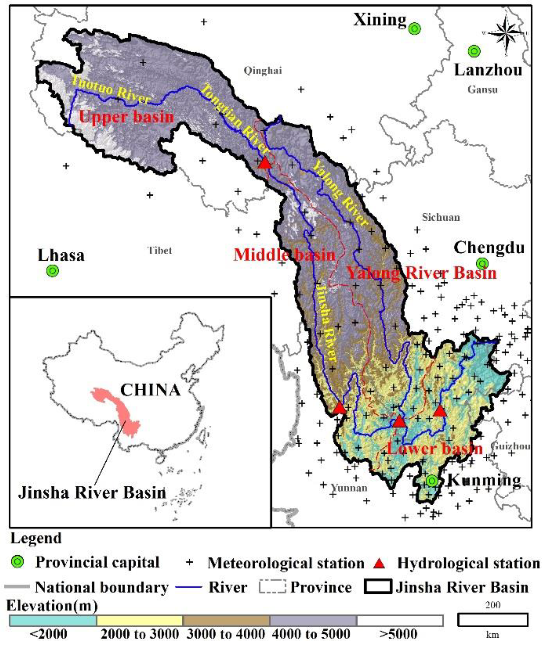
The Jinsha River Basin (JRB, 90°30′–105°15′ E and 24°36′–35°44′ N) is watershed of the upper Yibin city, covering an area of 473,200 km2 shared by four provinces and autonomous region (namely Qinghai, Tibet, Yunnan, Sichuan and Guizhou), is about 26% of the total drainage area of the Yangtze River Basin [8,13]. The Jinsha River is about 3464 km in length and originates from the peak of east Geladan Snowy Mountain in the Tanggula Mountains, flowing through Western Sichuan Plateau, Hengduan Mountains and Yunnan-Guizhou Plateau to the mountain area of Southwest Sichuan [14]. The Yalong River is the longest tributary of the JRB, with 1187 km in length (Figure 1). The mean annual temperature is 10.2 °C in the JRB. It increases progressively from northwest to southeast [13]. The general distribution of precipitation in JRB increases gradually from upstream to downstream. The annual average precipitation in the upper, middle and lower reaches is 350 mm, 600 mm and 1000 mm respectively [15]. The wet season lasts from June to October when 75 to 85% of total yearly rainfall happens. The average annual runoff is about 152 billion m3.
The JRB acts as an important water source in the west route of South-to-North Water Transfer Project. A total of 1.5 billion m3 of water will be transferred from the upper reaches of the Yalong River to the northern part of China in the first phase every year. The JRB also contributes to irrigation, water supply, flood control, wood drift, and tourism. Overall, the JRB plays a very important role in regional and national economic development.
2.2. A Brief Review of ArcSWAT Model
The ArcGIS10.2.2 interface of SWAT (ver.2012) was used in this study for water cycle simulation. It is a watershed-scale, process-based, continuous-time, and semi-distributed hydrological model, which can be used for predicting the impacts of climate change on the water hydrology of river basins [16]. The water balance equation which governs the hydrological components of SWAT model is given as:
where, SWti is soil water content at time t (mm H2O), SW0 is initial soil water content (mm H2O), t is simulation period (days), Rdayi is the amount of precipitation on the i-th day (mm H2O), Qsurfi is the amount of surface runoff on the i-th day (mm H2O), Eai is the amount of evapotranspiration on the i-th day (mm H2O), Wseepi is the amount of water entering the vadose zone from the soil profile on the i-th day (mm H2O) and Qgwi is the amount of baseflow on the i-th day (mm H2O).
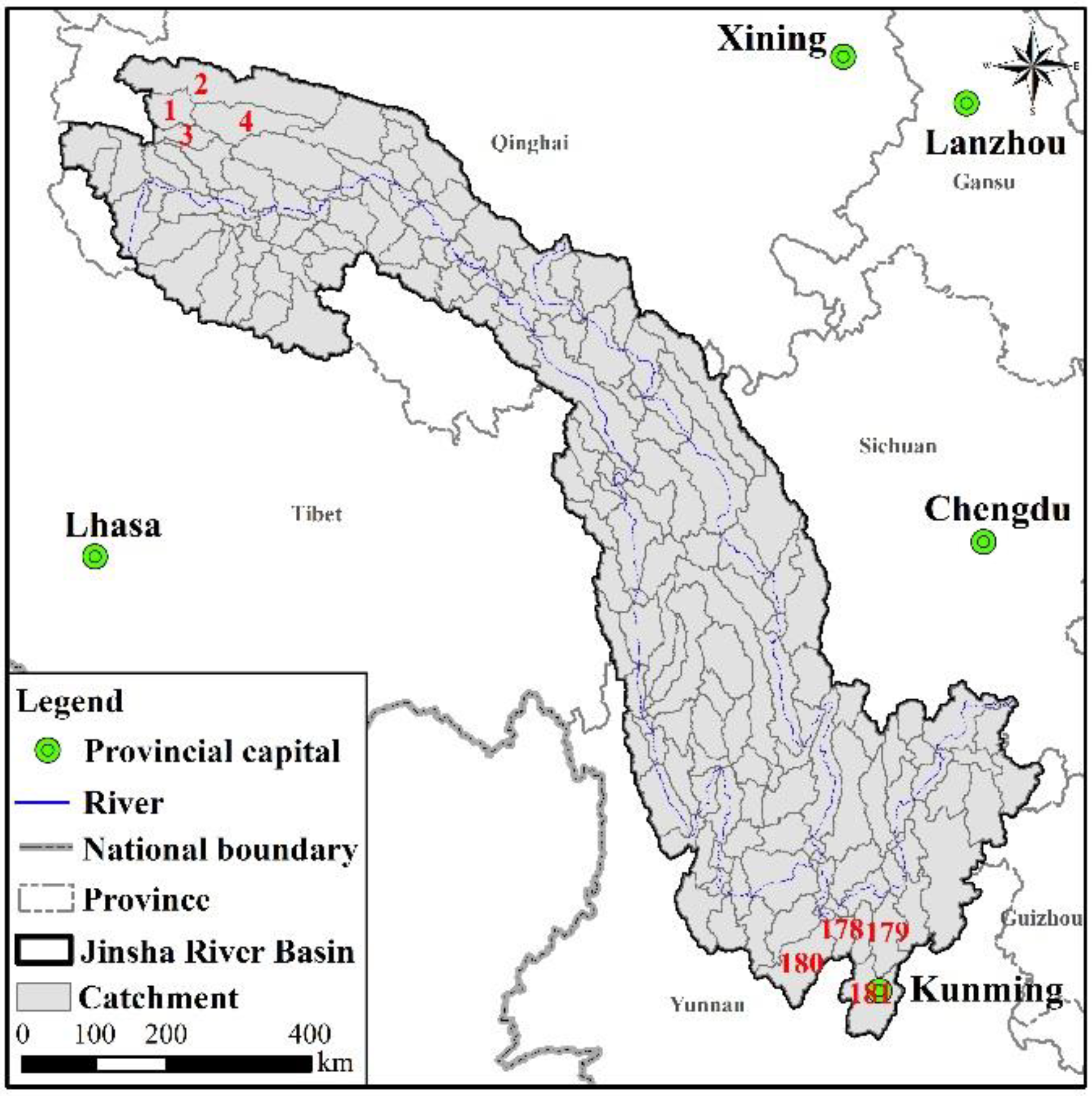
The JRB is comprised of 181 sub-basins which were divided into 579 Hydrological Response Units (HRUs) that satisfactorily represent watershed’s heterogeneity. In defining HRUs, 20% and 10% threshold values of land use and soil area have been considered to ignore minor land uses and soil types in each sub basin so as to avoid unnecessary large number of HRUs (Figure 2).
The coefficient of determination of the linear regression equation (R2) and the Nash-Sutcliffe efficiency coefficient (ENS) are chosen to assess the model’s feasibility in the study area [17]. The calculation formulas are as follows:
is observed depth of runoff (mm); is simulated depth of runoff(mm); and are the mean value of observed and simulated depth of runoff respectively(mm); n is the number of observed value. Models perform better with higher R2 and greater ENS. When ENs ≥ 0.75, it means the simulation is good; when 0.36 < ENS < 0.75, the simulation is basically good; when ENS ≤ 0.36, the simulation is poor [18].
2.3. Data
2.3.1. Observed Hydro-Meteorological Data
In this study, as the SWAT was used in water balance mode, the meteorological parameters which were considered to force the model were daily precipitation and the daily minimum and maximum temperature. The daily meteorological data during 1956 to 2013 from 196 meteorological stations in and around the JRB were collected for this study.
The observations used to evaluate the AR5 Climate Models’ simulated monthly precipitation and temperature are gridded monthly temperature and precipitation data prepared by the National Meteorological Information Center (NMIC) of the China Meteorological Administration (CMA) [19]. In this study, 208 grid boxes are selected to describe the areas of the JRB (Figure 3).
Streamflow data was collected from four hydrological stations in different parts of the JRB during the period from 1957 to 2012. It was used to analyze the runoff trend and sensitivity of streamflow to climate change, and to calibrate and validate the SWAT. The basic information of the four hydrological stations is listed in Table 1.
2.3.2. Future Climate Scenarios
The Inter-Sectoral Impact Model Intercomparison Project (ISI-MIP) [20] provides continuous daily-series meteorological data derived from GFDL-ESM2M, HADGEM2-ES, IPSL-CM5A-LR, MIROC-ESM-CHEM and NORESM1-M (Table 2), including historical scenario and future emission scenarios RCP 2.6, RCP4.5, RCP6.0 and RCP8.5. The data was bias-corrected and resampled by the ISI-MIP. It covers the period from 1960 to 2099 on a horizontal grid with 0.5° × 0.5° resolution [21]. The statistical characteristic of simulated data and observed data are consistent with each other. The spatial resolution of data can meet the requirements of hydrological simulation in the JRB. In this study, we used the three mitigation emissions scenarios (RCP2.6, RCP4.5, RCP8.5) and the period 2011–2050.
2.3.3. Digital Elevation Model, Land Use/Land Cover Map and Soil Map
The Digital Elevation Model (DEM) with a spatial resolution of 90 m was obtained from the CGIAR-CSI GeoPortal [22]. Land use/land cover map for 1980 and 2000 was obtained from the Data Center for Resources and Environmental Sciences, Chinese Academy of Sciences (Figure 4), and land use properties were directly from the SWAT model database. Soil map of JRB at a scale of 1:1,000,000 was procured from Institute of Soil Science, Chinese Academy of Sciences [23] (Figure 5).
2.4. Sensitivity Analysis of Runoff to Climate Change
In this study, we defined the sensitivity of streamflow to climate change as the proportional change of simulated streamflow by comparing their values with hypothetical climatic scenarios to their values with observed climatic data [24]. We consider the proportional change in precipitation and mean temperature as the factors contained by climate change. Then the sensitivity of streamflow to climate change could be defined as
where, P and T are precipitation and temperature; ΔP and ΔT are the hypothetical changes of precipitation and temperature; f(P,T) is the relation function between streamflow and climatic scenario; δ(ΔP,ΔT) is the sensitivity of streamflow to climate change. Based on the mean precipitation and temperature in the period 1961–1990 (baseline), precipitation is assumed to change by +30%, +20%, +10%, 0%, −10%, −20% and −30% in the future; temperature is assumed to change by +3 °C, +2 °C, +1 °C, 0 °C, −1 °C, −2 °C and −3 °C in the future [8].
2.5. Selection of Global Climate Model
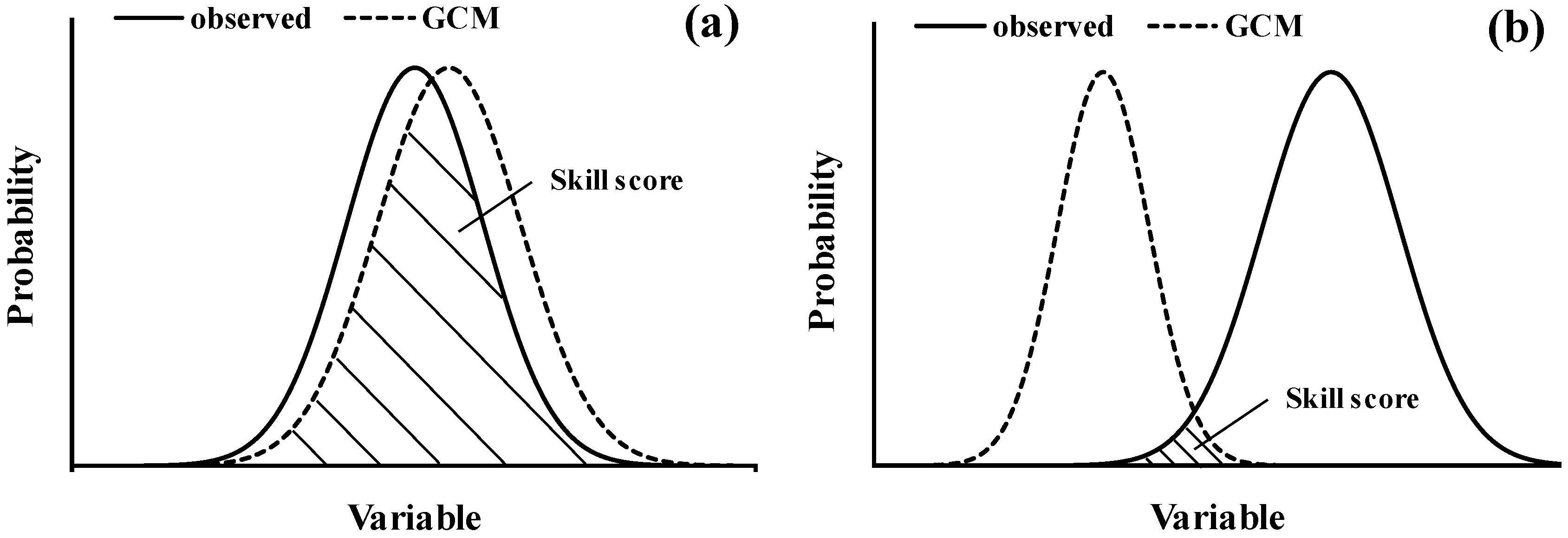
This study evaluated the coupled climate models and selected the relatively optimal GCMs for hydro-meteorological variability projection. The evaluation was focused on 4 regions of the JRB for the daily simulation of precipitation and temperature. It was based on probability density functions (PDFs). We defined an alternative metric to describe the similarity between two PDFs. This metric calculates the cumulative minimum value of two distributions of each binned value, thereby measuring the common area between two PDFs. The skill score (SS) can range between 0 and 1. SS is close to 1 when the model simulates the observed conditions perfectly (Figure 6a) and it is close to 0 when the overlap is negligible (Figure 6b) [12].
Expressed formally,
where n is the number of bins, Fsn is the frequency of values in a given bin from the model, and Fon is the frequency of values in a given bin from the observed data. SS was the summation of the minimum frequency values over all bins.
In this study, the monthly precipitation was fitted by a mixture function which was shown in Equation (6).
where, x represents a rainfall amount. G(x) is the mixture function. p is the probability of no rainfall. H(x) is step function, when x > 0, H(x) = 1, else H(x) = 0. F(x) is gamma cumulative probability function, the PDF is shown in Equation (7).
where, f(x) is the PDF. α is called the shape parameter and β is called the scale parameter. Γ(α) is gamma function.
The monthly average temperature was fitted by beta function. The PDF was shown in Equation (8).
where, x represents monthly average temperature. f(x) is the PDF. a, b, p and q are the parameters for beta function(B(p,q)).
Driven by the baseline daily climatology and the projected future daily climate data sets coming from the relatively optimal GCMs, the calibrated SWAT model can output the simulated daily streamflow in both baseline (1961 to 1990) and future period (2020 to 2050). Then the changes of future streamflow can be estimated.
3. Results and Discussion
3.1. Calibration and Verification
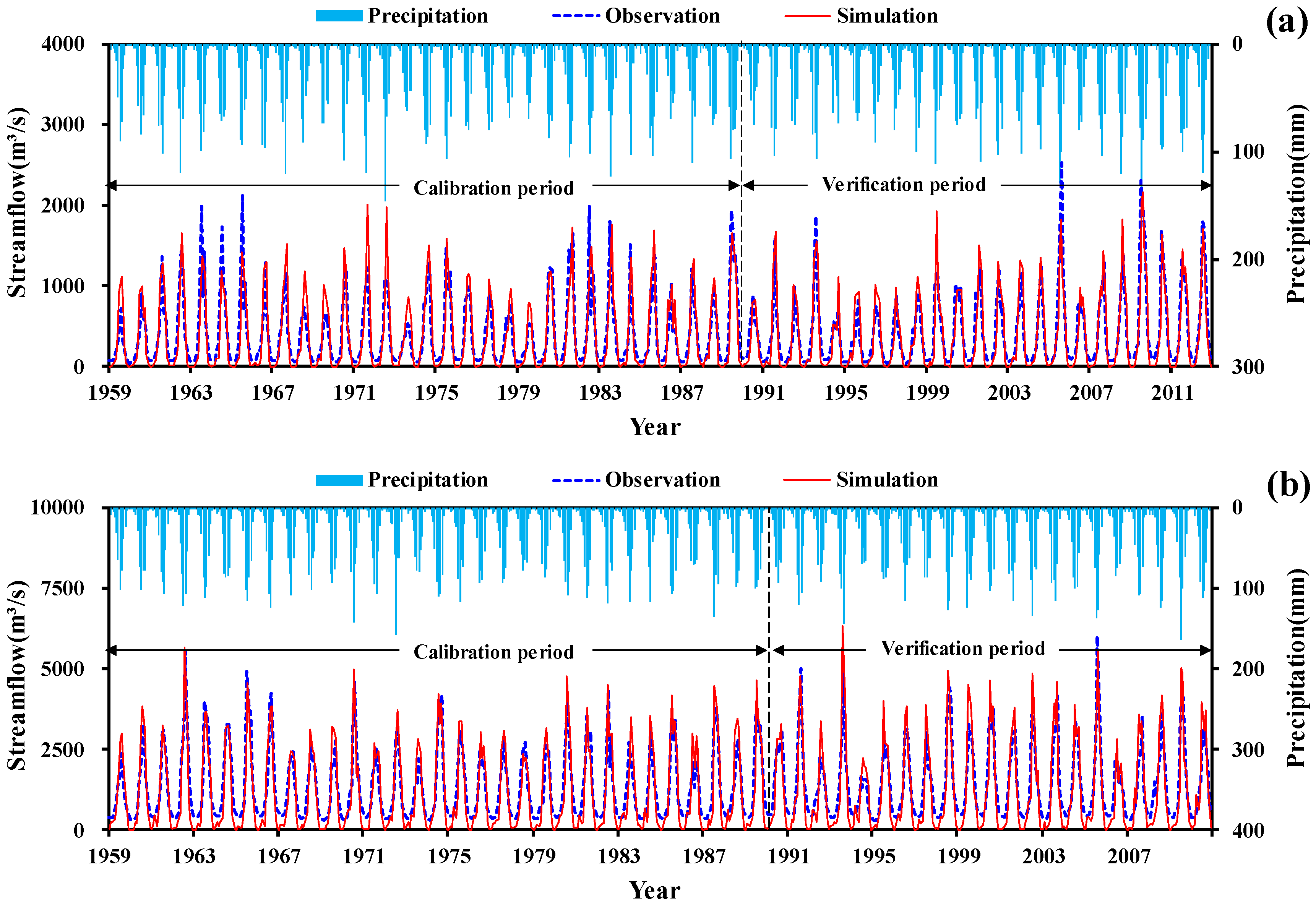
Table 3 summarized the performance of the SWAT in the four catchments. The ENS and R2 were higher than 0.8 in all catchments. Figure 7 showed the simulated and observed monthly streamflow in the calibration period and verification period. The results denoted good performance of the SWAT, although there were some differences between observation and simulation. Overall, the calibration and verification accuracy of the SWAT was acceptable for monthly streamflow simulation in the JRB.
3.2. Sensitivity of Streamflow to Climate Change
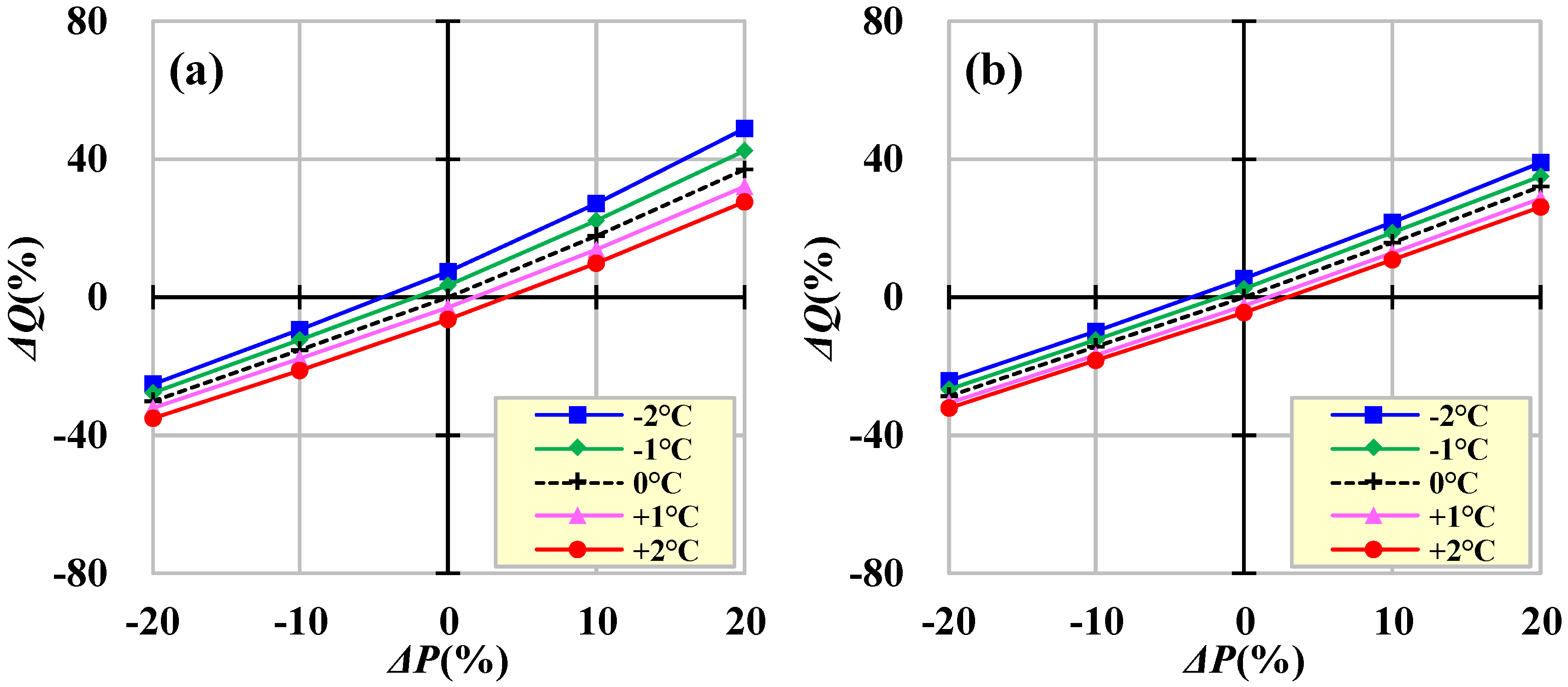
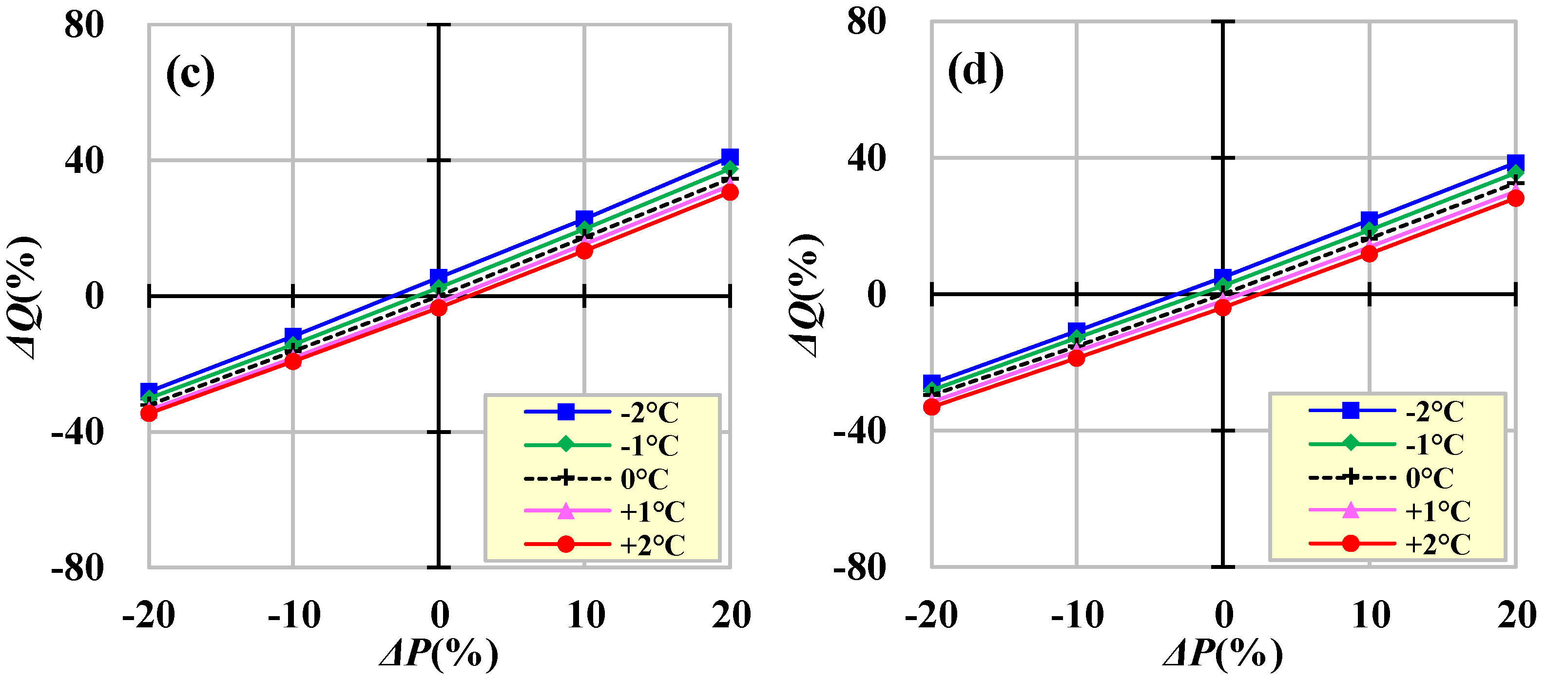
With the output of the SWAT using hypothetical climate scenarios, the sensitivity of runoff to climate change was estimated by Equation (5). Then the response of streamflow to changes of precipitation and temperature can be analyzed (shown in Figure 8 and Figure 9). In general, a rise in temperature would be a negative impact in streamflow due to higher evaporation and an increase in precipitation would certainly lead to higher streamflow.
Figure 8 showed the relation between ΔP (the changes in precipitation) and ΔQ (the changes in streamflow). It can be seen that a 10% precipitation increase might result in a streamflow increase of 15 to 18%. The responses of streamflow to temperature change were illustrated in Figure 9. From the figure we can find that a 1 °C increase in temperature will result in a 2 to 5% decrease in streamflow. Among 26 hypothetical climate scenarios, the precipitation in wettest scenario will increase by 30%, while the temperature will decrease by 3 °C. In addition, the precipitation in driest situation will decrease by 30%, while the temperature will increase by 3 °C. Under the wettest scenario, streamflow would be likely to change by 39 to 49%, while it might change by −35 to −33% under the driest scenario.
According to the study of Chiew, basins with higher runoff coefficients will be less sensitive to climatic changes [25]. If the runoff coefficient is more than 0.2 (high runoff coefficient), 10% decrease in precipitation may result in a 10 to 20% decrease in streamflow. While the same 10% decrease in precipitation may lead to a 40% decrease in streamflow in a basin with a low runoff coefficient. In Jinsha River Basin, the annual average runoff is 143 billion m3 (319.4mm) and the annual average precipitation is 592 mm. Therefore, the runoff coefficient in the JRB is about 0.54. It means that this basin should be less sensitive to climatic changes. Our results on the JRB are in accordance with this rule.
3.3. Assessment of Skill Score from GCMs’ Outputs and Changes in Precipitation and Temperature for 2020 to 2050 with the Output of the SWAT Using Hypothetical Climate Scenarios, the Sensitivity of Runoff to Climate Change
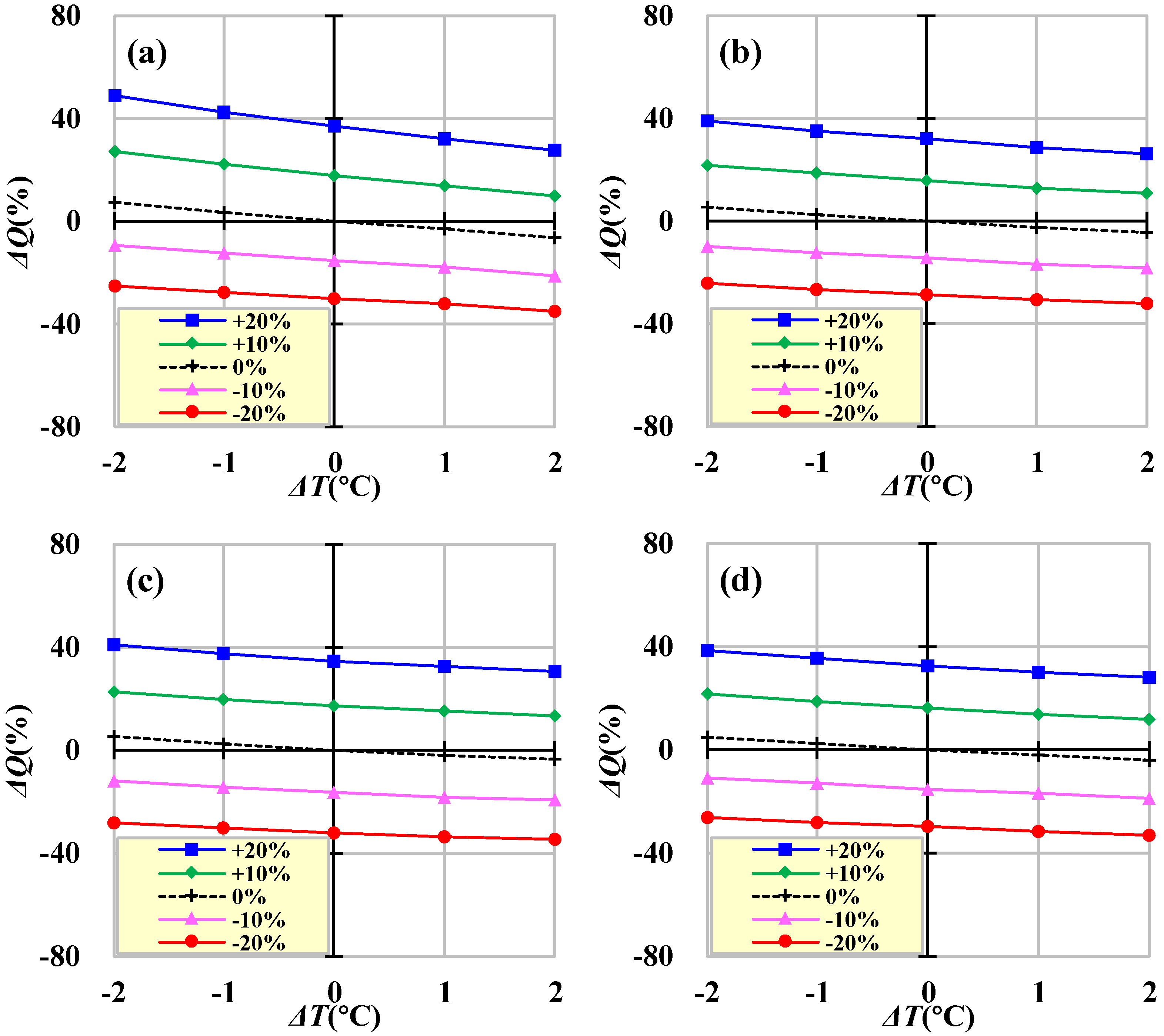
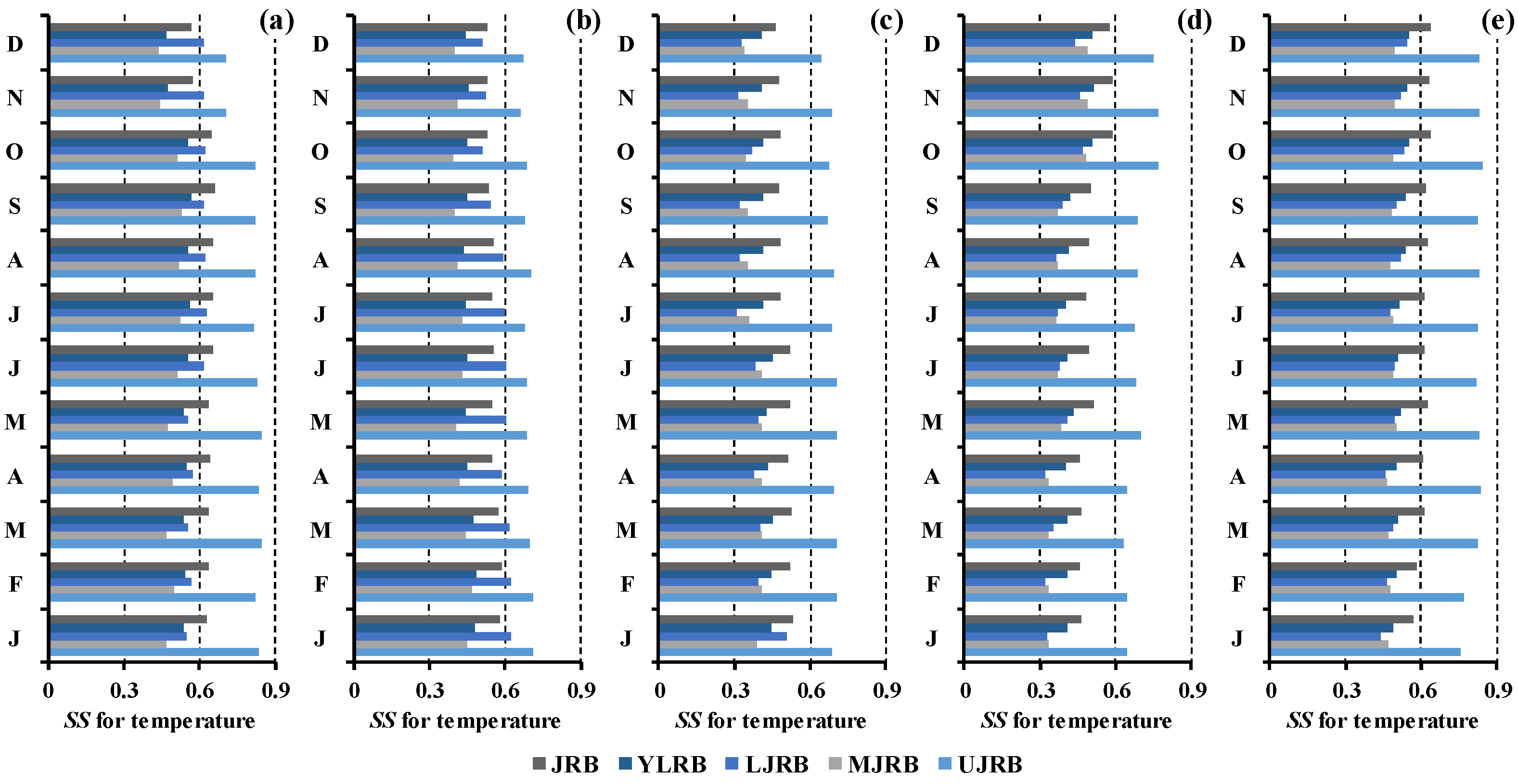
Figure 10 and Figure 11 showed the ensemble monthly skill score for each model averaged over all 4 regions defined in Figure 1. Because the outputs from five GCMs in this study have been bias-corrected by ISI-MIP, the SSs for precipitation and temperature simulation were not low. The SSs averaged over the JRB were more than 0.46. However, there still exists some difference among GCMs or variables. The averaged SSs over the JRB and all 12 months for precipitation were between 0.63 and 0.68. However, these averaged SSs for temperature were between 0.50 to 0.63 and the SSs for 3 of the 5 models were less than 0.6. These models were HadGEM2-ES, IPSL-CM5A-LR and MIROC-ESM-CHEM. Based on the above analysis, we considered GFDL-ESM2M and NORESM1-M as the relatively optimal GCMs in simulating the precipitation and temperature in the JRB. The outputs came from these two GCMs were chosen for the analysis of future climate change and its effects on streamflow.
The precipitation and temperature are the two main factors driving SWAT model. The changes in precipitation and temperature will directly affect the change in streamflow simulated by SWAT. Thus, we would firstly analyze changes in precipitation and temperature for the baseline (1961 to 1990) to the projection period (2020 to 2050). To eliminate the impacts of systematic deviation in GCMs on precipitation and temperature projection in the future, relative change between simulated value in projection period and that in baseline was chosen to reveal the evolution trend. To reduce the uncertainty from GCMs, we only used the relatively optimal GCMs (GFDL-ESM2M and NORESM1-M) to analysis the changes in precipitation and temperature in the future period.
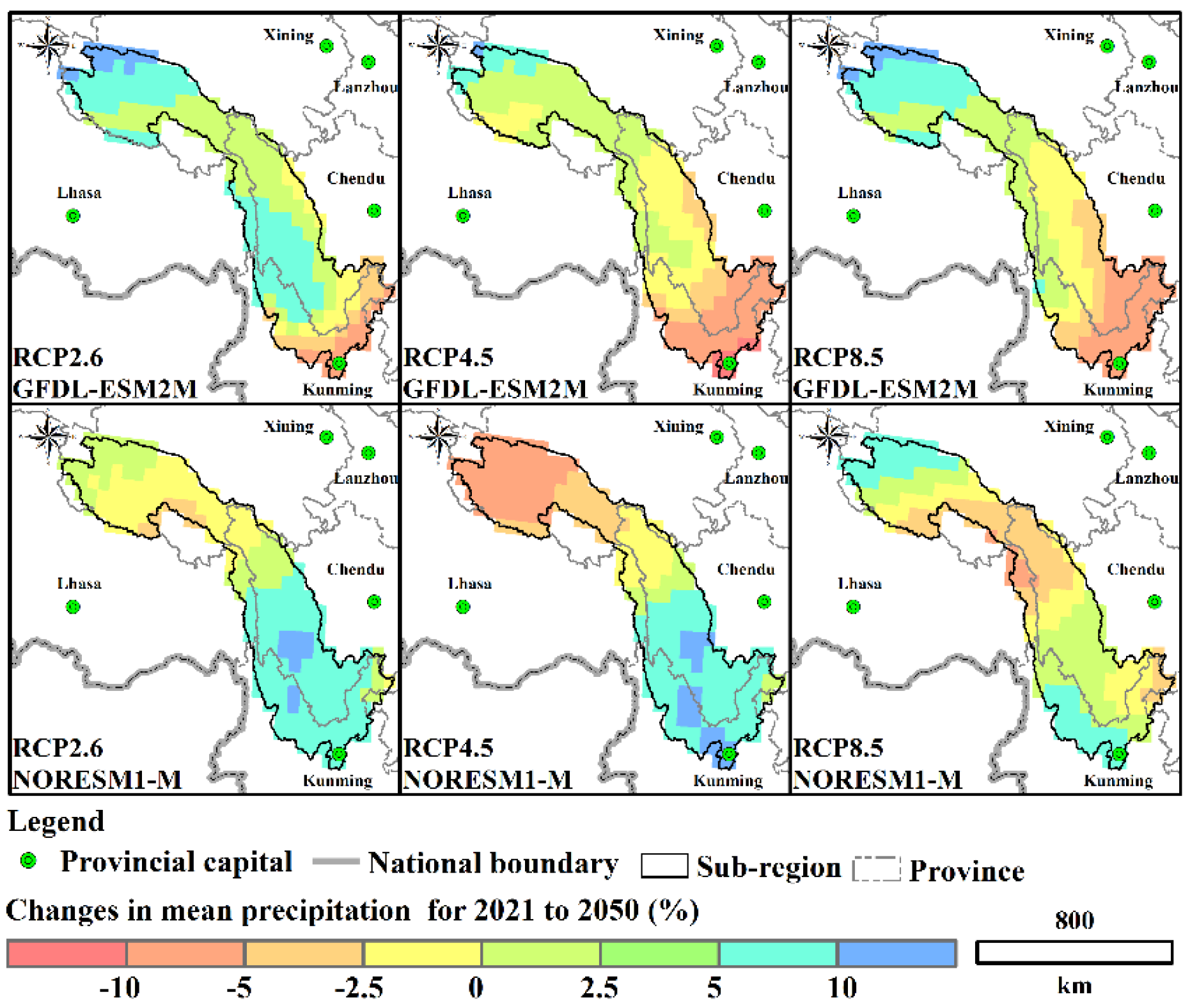
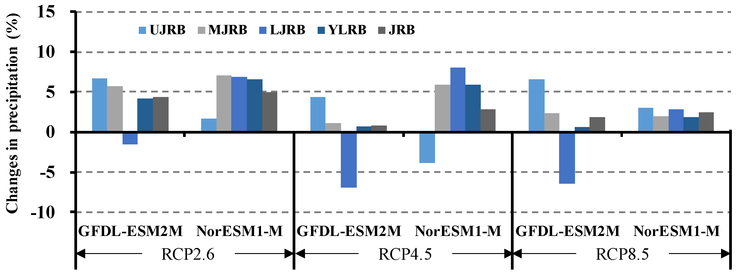
Figure 12 and Figure 13 showed the relative changes in mean annual precipitation simulated by the relatively optimal GCMs between RCP2.5, RCP4.5 and RCP8.5 when compared with that of the baseline. The spatial pattern was different in GFDL-ESM2M and NORESM1-M. GFDL-ESM2M suggested that the precipitation would increase in the upper and middle Jinsha River Basin (UMJRB), but decrease in the lower basin (LJRB). Future precipitation changes in the UJRB, MJRB, YLRB and LJRB were projected to be 4.3 to 6.7%, 1.1 to 5.7%, 0.6 to 4.2% and −6.9 to −1.5%, respectively. However, the spatial characteristics of changes in annual precipitation predicted by NORESM1-M were different from GFDL-ESM2M. Large increases in precipitation covered the LJRB throughout the projection period. The precipitation was likely to increase by 2.8 to 8.1% in this area. However, it would change slightly in the whole JRB by only 0.8 to 5.0%.
Models have a variable performance in simulating precipitation and temperature. Limited by the complexity of climate models and existing methods, only one or several indices (e.g., skill score) can be used to evaluate the simulation effect. So the SS in UJRB is higher than the SS in the other regions, but it is hard to explain from the aspects of climate model structure why a certain climate model has better simulation of precipitation or temperature in some certain places. Further research will be done to improve this issue.
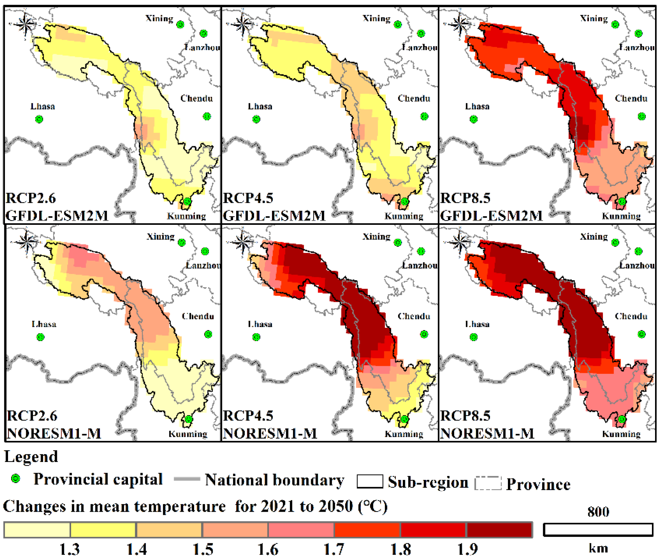
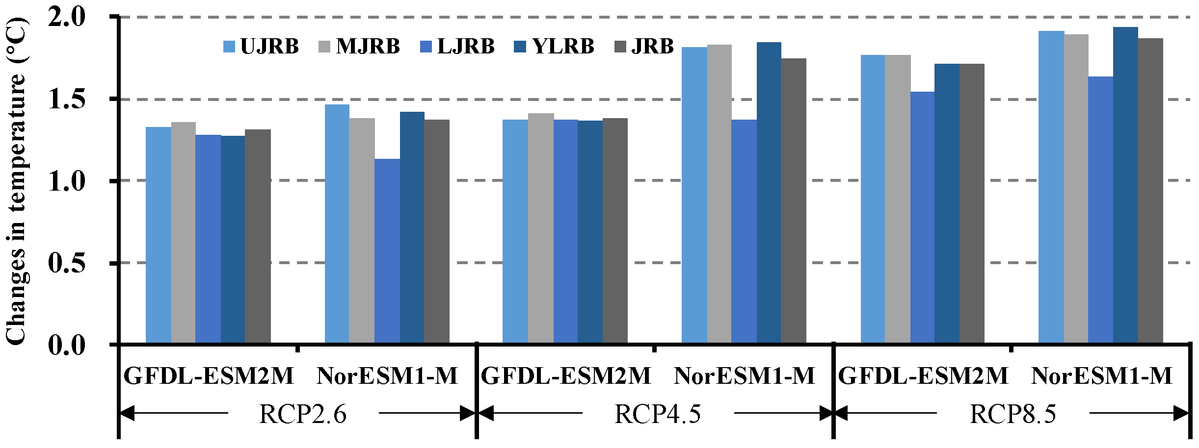
Figure 14 and Figure 15 illustrated the absolute change in annual mean temperature in the future period. The spatial pattern was almost the same in multiple GCM-scenario combinations, but the magnitude varied considerably. Extreme warming was more widespread in NORESM1-M than in GFDL-ESM2M, particularly under RCP4.5. The larger warming was projected in the UMJRB. The annual mean temperature over the UMJRB was predicted to increase by more than 1.77 °C in RCP8.5 scenario. In the future period, the temperature would increase by 1.31 to 1.38 °C for RCP2.6, 1.38 to 1.75 °C for RCP4.5 and 1.72 to 1.87 °C for RCP8.5.
3.4. Changes in Streamflow for 2020 to 2050
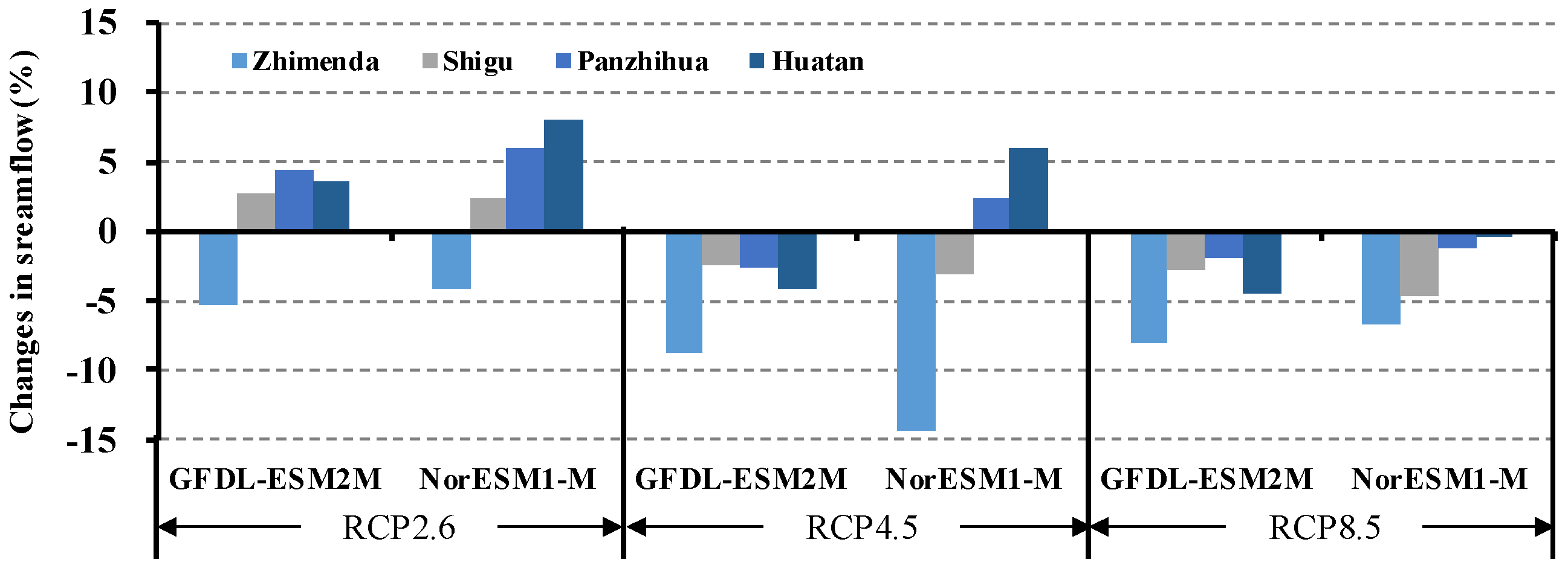
Using GFDL-ESM2M and NORESM1-M-projected daily precipitation and temperature under the three RCP scenarios, the SWAT model was run on the JRB from 1961 to 2050. Because it is hard to project future human activities (e.g., land use), the anthropogenic effects were not taken into consideration in projection of future streamflow changes. All parameters of the SWAT model were kept with no change. With the outputs from the SWAT model, the changes in streamflow for period 2020 to 2050 were statistically analyzed. Results showed that different GCM-scenario combinations were associated with different changes in streamflow, resulting in opposite conclusions. Taking Huatan Station as an example, GFDL-ESM2M projected 4.2% streamflow decrease for the future period under RCP4.5, while NORESM1-M estimated 6.0% increase in streamflow for the same period and climate scenario. However, projected trends from the different GCMs were the same under RCP2.6 and RCP8.5. The streamflow in Zhimenda was projected to decrease by 4.1 to 5.2% under RCP2.6 and 6.6 to 8.1% under RCP8.5. The streamflow in the MLJRB (Shigu, Panzhihua and Huatan) was likely to increase by 2.4 to 8.1% under RCP2.6, but was excepted to increase by 0.3 to 4.5% in the same region under RCP8.5 (Figure 16).
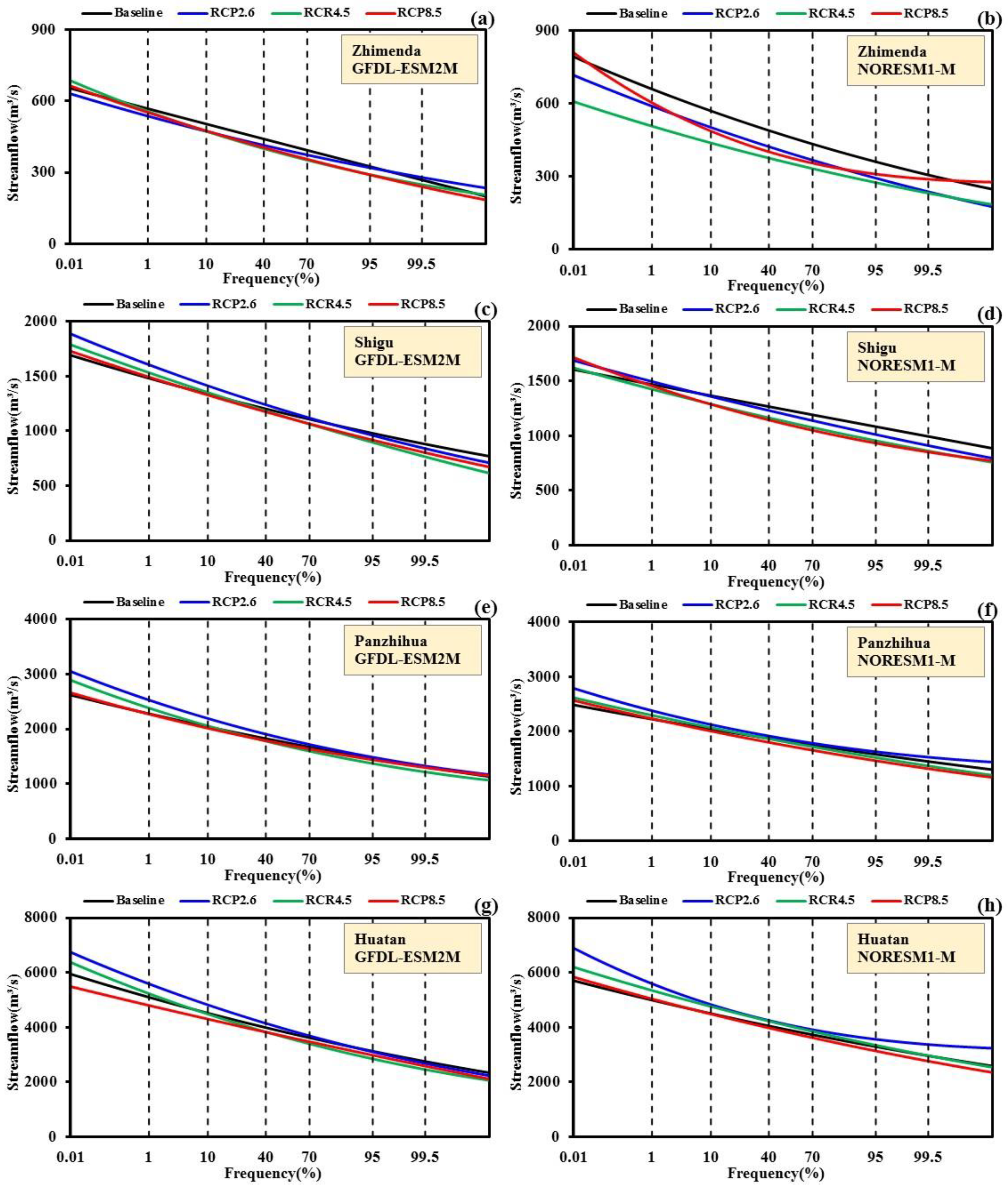
To compare the frequency of annual mean streamflow between baseline and future period, P-III frequency distributions were illustrated for comparison (Figure 17). When the frequency is less than 10%, RCP2.6 and RCP4.5 scenarios suggested a rather similar increasing trend in the MLJRB (Shigu, Panzhihua and Huatan). The opposite trend was found in the same region under 8.5 scenario. To further investigate the changes in streamflow, three different frequencies (P = 90%, P = 50% and P = 10%) were chosen (Table 4). As shown in Table 4, the low streamflow (P = 90%, Q90), median streamflow (P = 50%, Q50) and higher streamflow (P = 10%, Q10) in Zhimenda were projected to decrease in all the climate change scenarios. The largest percentage decreases in these three kinds of streamflow were mainly found for NORESM1-M. In Shigu station, nearly all the climate change scenarios showed that the Q90 and Q50 would likely to decrease, but there was a relatively large uncertainty in the projection of Q10. One of the six scenarios projected that the Q10 would increase by 5%. Two of the scenarios projected that the Q10 would decrease by 5%. The rest scenarios projected no significant change. The Q90 will increase slightly in Panzhihua and Huatan under RCP2.6 while may decrease under RCP4.5 and RCP8.5. The Q10 will increase in the same stations under RCP2.6. However, the changes in Q10 under RCP4.5 and RCP8.5 were not obvious.
4. Discussion and Conclusions
Based on five CMIP5 CMs, this study discussed the changes in projected streamflow of the JRB under RCP2.6, RCP4.5 and RCP8.5 scenarios. The SWAT model was employed to simulate monthly streamflow, using observed meteorological data from NMIC and the ISI-MIP climate dataset.
Observed monthly streamflow at four stations in the JRB was used for calibration and validation of the SWAT model. The model performed well in simulating monthly streamflow in the JRB, with ENS and R2 higher than 0.8 in the four catchments. This demonstrated that calibrated model can be used to estimate the impact of climate change on future streamflow in the JRB.
The study of Chiew revealed that the sensitivity of a river basin to changes in precipitation and temperature was strongly related to the runoff coefficient [24]. The basin with higher runoff coefficient is less sensitivity to climate change. The JRB is in this category. In this study, area, a 10% precipitation decrease might result in a streamflow increase of 15 to 18% and a 1 °C increase in temperature might results in a 2 to 5% decrease in streamflow.
The skill of the selected five GCMs was assessed using a skill score (SS) based on the overlap between the observed and simulated PDFs (grid by grid) in the baseline (1961 to 1990). In general, GFDL-ESM2M and NORESM1-M showed considerable skill in representing the observed PDFs of monthly precipitation and temperature. The averaged SSs over the JRB and all 12 months for precipitation and temperature were more than 0.6. Therefore, GFDL-ESM2M and NORESM1-M can be chosen as the relatively optimal GCMs to analysis the changes in precipitation and temperature and their effects on streamflow in the future period.
In the future period, the precipitation was projected to increase slightly in the whole JRB by only 0.8 to 5.0%. While the temperature was likely to increase significantly. It would increase by 1.31 to 1.38 °C for RCP2.6, 1.38 to 1.75 °C for RCP4.5 and 1.72 to 1.87 °C for RCP8.5. The projected changes in mean annual streamflow were generally similar under RCP2.6 and RCP8.5. The streamflow was projected to decrease in the UJRB (Zhimenda) while it was excepted to increase in the MLJRB (Shigu, Panzhihua and Huatan). However, all the changes (increase or decrease) were less than 10%. The projections of future mean annual streamflow carried high uncertainty under RCP4.5. The different GCMs were associated with different changes in mean annual streamflow, resulting in opposite conclusions. When considering the results from three future scenarios of the two relatively optimal GCMs, the range of relative changes in the UJRB and the MLJRB was 4.1 to 14.3% and −4.6 to 8.1%, respectively. The low streamflow, median streamflow and higher streamflow were projected to change more obvious in the Zhimenda and Shigu than other stations. These three kinds of streamflow in Zhimenda were projected to decrease in all the climate change scenarios. In Shigu station, nearly all the climate change scenarios showed that the low streamflow and median streamflow would likely to decrease, but there was a relatively large uncertainty in the projection of higher streamflow. In the MLJRB, the changes of low streamflow for 2020 to 2050 were between −5.8 to 7.4%. Therefore, the potential impact of climate on streamflow will have little effect on the planning and management of the west route of SNWTP.
This research chose SWAT model to do hydrological simulation. Hydrologic model is likely to cause less error (or uncertainty) than the climate projections. However, compared with physics-based hydrological models, transferring the calibration of model parameters under historical conditions to futures with different climatic characteristics raises questions of validity [26,27]. In future research, different kinds of hydrological models coupled with more GCMs will be added to do uncertainty analysis.
Author Contributions
J.Y., Z.Y. (Zhe Yuan) and Z.Y. (Zhiyong Yang) worked together in forming ideas of this paper; J.Y. and Z.Y. (Zhe Yuan) worked together in calculating and writing of this manuscript; Y.W. carried out the calculation and analysis of runoff in the study area; D.Y. and Z.Y. (Zhiyong Yang) provided supervision during the whole process.
Funding
This research was funded by [National Key Research and Development Project] grant number [2017YFC1502404]; [the Open Research Fund of State Key Laboratory of Simulation and Regulation of Water Cycle in River Basin(China Institute of Water Resources and Hydropower Research)] grant number [IWHR-SKL-KF201804]; [National Natural Science Foundation of China] grant number [51779013, 51709008]; [National Public Research Institutes for Basic R&D Operating Expenses Special Project] grant number [CKSF2017029].
Conflicts of Interest
The authors declare no conflict of interest. The founding sponsors had no role in the design of the study; in the collection, analyses, or interpretation of data; in the writing of the manuscript, and in the decision to publish the results.
References
- IPCC. Climate Change 2013: The Physical Science Basis; Cambridge University Press: Cambridge, UK, 2013. [Google Scholar]
- Arnell, N.W. Climate change and global water resources. Glob. Environ. Chang. 1999, 9, 31–49. [Google Scholar] [CrossRef]
- Huntington, J.; Mcgwire, K.; Morton, C.; Snyder, K.; Peterson, S.; Erickson, T.; Niswonger, R.; Carroll, R.; Smith, G.; Allen, R. Assessing the role of climate and resource management on groundwater dependent ecosystem changes in arid environments with the Landsat archive. Remote Sens. Environ. 2016, 185, 186–197. [Google Scholar] [CrossRef]
- Thodsen, H. The influence of climate change on stream flow in Danish rivers. J. Hydrol. 2007, 333, 226–238. [Google Scholar] [CrossRef]
- Githui, F.; Gitau, W.; Mutua, F.; Bauwens, W. Climate change impact on SWAT simulated streamflow in western Kenya. Int. J. Climatol. 2009, 29, 1823–1834. [Google Scholar] [CrossRef] [Green Version]
- Chien, H.; Yeh, P.J.F.; Knouft, J.H. Modeling the potential impacts of climate change on streamflow in agricultural watersheds of the Midwestern United States. J. Hydrol. 2013, 491, 73–88. [Google Scholar] [CrossRef]
- Eisner, S.; Flörke, M.; Chamorro, A.; Daggupati, P.; Donnelly, C.; Huang, J.; Hundecha, Y.; Koch, H.; Kalugin, A.; Krylenko, I.; et al. An ensemble analysis of climate change impacts on streamflow seasonality across 11 large river basins. Clim. Chang. 2017, 141, 401–417. [Google Scholar] [CrossRef]
- Yuan, Z.; Yan, D.; Yang, Z.; Yin, J.; Zhang, C.; Yuan, Y. Projection of surface water resources in the context of climate change in typical regions of China. Hydrol. Sci. J. 2017, 62, 283–293. [Google Scholar] [CrossRef]
- Bollasina, M.; Nigam, S. Indian Ocean SST, evaporation, and precipitation during the South Asian summer monsoon in IPCC-AR4 coupled simulations. Clim. Dyn. 2009, 33, 1017–1032. [Google Scholar] [CrossRef]
- Anandhi, A.; Nanjundiah, R.S. Performance evaluation of AR4 Climate Models in simulating daily precipitation over the Indian region using skill scores. Theor. Appl. Climatol. 2015, 119, 551–566. [Google Scholar] [CrossRef]
- Yin, J.; Yan, D.; Yang, Z.; Yuan, Z.; Yuan, Y.; Zhang, C. Projection of extreme precipitation in the context of climate change in Huang-Huai-Hai region, China. J. Earth Syst. Sci. 2016, 125, 417–429. [Google Scholar] [CrossRef]
- Perkins, S.E.; Pitman, A.J.; Holbrook, N.J.; McAneney, J. Evaluation of the AR4 climate models’ simulated daily maximum temperature, minimum temperature, and precipitation over Australia using probability density functions. J. Clim. 2007, 20, 4356–4376. [Google Scholar] [CrossRef]
- Wang, H. The Future Situation of Water Resources in China and its Management Requirements. World Environ. 2011, 2, 16–17. [Google Scholar]
- Liu, H.; Lan, H.; Liu, Y.; Zhou, Y. Characteristics of spatial distribution of debris flow and the effect of their sediment yield in main downstream of Jinsha River, China. Environ. Earth Sci. 2011, 64, 1653–1666. [Google Scholar] [CrossRef]
- Chen, Y.; Wang, W.; Wang, G.; Wang, S. Characteristics analysis on temperature and precipitation variation in Jinsha River Basin. Plateau Mt. Meteorol. Res. 2010, 30, 51–56. [Google Scholar]
- Uniyal, B.; Jha, M.K.; Verma, A.K. Assessing climate change impact on water balance components of a river basin using SWAT model. Water Resour. Manag. 2015, 29, 4767–4785. [Google Scholar] [CrossRef]
- Nash, J.E.; Sutclife, J.V. River low forecasting through conceptual models—Part I: A discussion of principles. J. Hydrol. 1970, 10, 282–290. [Google Scholar] [CrossRef]
- Motovilov, Y.G.; Gottschalk, L.; Engeland, K.; Rodhe, A. Validation of a distributed hydrological model against spatial observations. Agric. For. Meteorol. 1999, 98, 257–277. [Google Scholar] [CrossRef]
- NMIC (National Meteorological Information Center). Assessment Report of China’s Ground Precipitation 0.5° × 0.5° Gridded Dataset (V2.0); National Meteorological Information Center of China: Beijing, China, 2012. [Google Scholar]
- The Inter-Sectoral Impact Model Intercomparison Project. Available online: https://isimip.org/ (accessed on 5 June 2018).
- Warszawski, L.; Frieler, K.; Huber, V.; Piontek, F.; Serdeczny, O.; Schewe, J. The Inter-Sectoral Impact Model Intercomparison Project (ISI–MIP): Project framework. Proc. Natl. Acad. Sci. USA 2014, 111, 3228–3232. [Google Scholar] [CrossRef] [PubMed]
- The CGIAR Consortium for Spatial Information. Available online: http://srtm.csi.cgiar.org/ (accessed on 5 June 2018).
- China Soil Information Service Platform. Available online: http://www.soil.csdb.cn (accessed on 5 June 2018).
- Bao, Z.; Zhang, J.; Liu, J.; Wang, G.; Yan, X.; Wang, X.; Zhang, L. Sensitivity of hydrological variables to climate change in the Haihe River basin, China. Hydrol. Process. 2012, 26, 2294–2306. [Google Scholar] [CrossRef]
- Chiew, F.H.S. Estimation of rainfall elasticity of streamflow in Australia. Hydrol. Sci. J. 2006, 51, 613–625. [Google Scholar] [CrossRef] [Green Version]
- Coron, L.; Andréassian, V.; Perrin, C.; Lerat, J.; Vaze, J.; Bourqui, M.; Hendrickx, F. Crash testing hydrological models in contrasted climate conditions: An experiment on 216 Australian catchments. Water Resour. Res. 2012, 48, 213–223. [Google Scholar] [CrossRef]
- Guerreiro, S.B.; Birkinshaw, S.; Kilsby, C.; Fowler, H.J.; Lewis, E. Dry getting drier—The future of transnational river basins in Iberia. J. Hydrol. Reg. Stud. 2017, 12, 238–252. [Google Scholar] [CrossRef]
Figure 1.
Location of Jinsha River Basin.

Figure 2.
The catchments divided by SWAT.

Figure 3.
Grid boxes in the JRB.

Figure 4.
The Landuse of JRB in 1980 (a) and 2000 (b).

Figure 5.
Soil distribution in JRB.

Figure 6.
Diagrams of GCM vs observed PDF illustrating the total skill score in (a) a near-perfect skill score and (b) a very poor skill score.
Figure 6.
Diagrams of GCM vs observed PDF illustrating the total skill score in (a) a near-perfect skill score and (b) a very poor skill score.

Figure 7.
Simulated and observed monthly discharge during the calibration period and the verification period: (a) Zhimenda catchment; (b) Shigu catchment; (c) Panzhihua catchment; (d) Huatan catchment.
Figure 7.
Simulated and observed monthly discharge during the calibration period and the verification period: (a) Zhimenda catchment; (b) Shigu catchment; (c) Panzhihua catchment; (d) Huatan catchment.


Figure 8.
Sensitivity on mean streamflow due to mean precipitation change in JRB: Zhimenda (a); Shigu (b); Panzhihua (c); and Huatan (d).
Figure 8.
Sensitivity on mean streamflow due to mean precipitation change in JRB: Zhimenda (a); Shigu (b); Panzhihua (c); and Huatan (d).


Figure 9.
Sensitivity on mean streamflow due to mean temperature change in JRB: Zhimenda (a); Shigu (b); Panzhihua (c); and Huatan (d).
Figure 9.
Sensitivity on mean streamflow due to mean temperature change in JRB: Zhimenda (a); Shigu (b); Panzhihua (c); and Huatan (d).

Figure 10.
Skill score for precipitation simulation: GFDL-ESM2M (a); HADGEM2-ES (b); IPSL-CM5A-LR (c); MIROC-ESM-CHEM (d); NORESM1-M (e).
Figure 10.
Skill score for precipitation simulation: GFDL-ESM2M (a); HADGEM2-ES (b); IPSL-CM5A-LR (c); MIROC-ESM-CHEM (d); NORESM1-M (e).

Figure 11.
Skill score for temperature simulation: GFDL-ESM2M (a); HADGEM2-ES (b); IPSL-CM5A-LR (c); MIROC-ESM-CHEM (d); NORESM1-M (e).
Figure 11.
Skill score for temperature simulation: GFDL-ESM2M (a); HADGEM2-ES (b); IPSL-CM5A-LR (c); MIROC-ESM-CHEM (d); NORESM1-M (e).

Figure 12.
Changes in mean precipitation for 2021 to 2050.

Figure 13.
Changes in mean precipitation for 2021 to 2050 in different regions.

Figure 14.
Changes in mean temperature for 2021 to 2050.

Figure 15.
Changes in temperature for 2021 to 2050 in different regions.

Figure 16.
Changes in mean streamflow for 2021 to 2050 in different stations.

Figure 17.
PIII frequency distribions of annual mean streamflow in Zhimenda (a,b), Shigu (c,d), Panzhihua (e,f) and Huatan (g,h) under different climate change scenarios.
Figure 17.
PIII frequency distribions of annual mean streamflow in Zhimenda (a,b), Shigu (c,d), Panzhihua (e,f) and Huatan (g,h) under different climate change scenarios.


Table 1.
Basic information of the 4 hydrological stations.
| Hydrological Station | River | Lon. (E°) | Lat. (N°) | Catchment Area (103 km2) | Area Percent (%) | Data Period |
|---|---|---|---|---|---|---|
| Zhimenda | Tongtian River | 97.24 | 33.01 | 159.8 | 32.4 | 1957–2012 |
| Shigu | Jinsha River | 99.96 | 26.87 | 234.1 | 47.4 | 1956–2010 |
| Panzhihua | Jinsha River | 101.72 | 26.58 | 280.9 | 56.9 | 1966–2000 |
| Huatan | Jinsha River | 102.88 | 26.88 | 447.7 | 90.7 | 1977–2000 |
Table 2.
List of general circulation models (GCMs) used in this study.
| Centre | Country | Name |
|---|---|---|
| Geophysical Fluid Dynamics Laboratory (GFDL) | United States | GFDL-ESM2M |
| Hadley Centre for Climate Prediction and Research, Met Office | United Kingdom | HADGEM2-ES |
| L’Institut Pierre-Simon Laplace (IPSL) | France | IPSL-CM5A-LR |
| Technology, Atmosphere and Ocean Research Institute, and National Institute for Environmental Studies | Japan | MIROC-ESM-CHEM |
| Norwegian Climate Centre | Norway | NORESM1-M |
Table 3.
Performance of the SWAT for monthly streamflow simulation in the Zhimenda, Shigu, Panzhihua and Huatan catchment.
Table 3.
Performance of the SWAT for monthly streamflow simulation in the Zhimenda, Shigu, Panzhihua and Huatan catchment.
| Catchment | Period | Year | ENS | R2 |
|---|---|---|---|---|
| Zhimenda | Calibration period | 1959–1990 | 0.80 | 0.84 |
| Verification period | 1991–2012 | 0.88 | 0.91 | |
| Shigu | Calibration period | 1959–1990 | 0.82 | 0.91 |
| Verification period | 1991–2010 | 0.80 | 0.93 | |
| Panzhihua | Calibration period | 1966–1990 | 0.85 | 0.92 |
| Verification period | 1991–2000 | 0.88 | 0.93 | |
| Huatan | Calibration period | 1977–1990 | 0.90 | 0.95 |
| Verification period | 1991–2000 | 0.93 | 0.96 |
Table 4.
Percentage changes (%) in streamflow under different scenarios.
| Frequency | Scenario | Zhimenda | Shigu | Panzhihua | Huatan | |
|---|---|---|---|---|---|---|
| P = 90% | RCP2.6 | GFDL-ESM2M | −3.0 | −1.0 | 1.6 | 0.0 |
| NORESM1-M | −17.4 | −6.0 | 2.5 | 6.6 | ||
| RCP4.5 | GFDL-ESM2M | −10.8 | −7.0 | −6.0 | −8.1 | |
| NORESM1-M | −23.5 | −11.2 | −3.1 | 2.1 | ||
| RCP8.5 | GFDL-ESM2M | −10.6 | −5.4 | −2.1 | −4.3 | |
| NORESM1-M | −16.0 | −13.4 | −6.8 | −4.2 | ||
| P = 50% | RCP2.6 | GFDL-ESM2M | −5.8 | 2.4 | 3.8 | 3.2 |
| NORESM1-M | −14.1 | −3.3 | 2.2 | 4.8 | ||
| RCP4.5 | GFDL-ESM2M | −9.8 | −2.3 | −3.3 | −4.7 | |
| NORESM1-M | −23.2 | −8.6 | −0.8 | 4.0 | ||
| RCP8.5 | GFDL-ESM2M | −8.6 | −2.7 | −2.2 | −4.1 | |
| NORESM1-M | −18.2 | −10.5 | −4.3 | −2.1 | ||
| P = 10% | RCP2.6 | GFDL-ESM2M | −6.2 | 5.7 | 7.4 | 6.7 |
| NORESM1-M | −11.9 | −0.5 | 4.1 | 7.3 | ||
| RCP4.5 | GFDL-ESM2M | −6.1 | 1.2 | 0.7 | −0.8 | |
| NORESM1-M | −23.1 | −5.6 | 1.4 | 5.7 | ||
| RCP8.5 | GFDL-ESM2M | −5.7 | −0.6 | −1.4 | −4.8 | |
| NORESM1-M | −14.5 | −5.8 | −1.7 | −0.4 | ||
© 2018 by the authors. Licensee MDPI, Basel, Switzerland. This article is an open access article distributed under the terms and conditions of the Creative Commons Attribution (CC BY) license (http://creativecommons.org/licenses/by/4.0/).
Share and Cite
MDPI and ACS Style
Yin, J.; Yuan, Z.; Yan, D.; Yang, Z.; Wang, Y. Addressing Climate Change Impacts on Streamflow in the Jinsha River Basin Based on CMIP5 Climate Models. Water 2018, 10, 910. https://doi.org/10.3390/w10070910
AMA Style
Yin J, Yuan Z, Yan D, Yang Z, Wang Y. Addressing Climate Change Impacts on Streamflow in the Jinsha River Basin Based on CMIP5 Climate Models. Water. 2018; 10(7):910. https://doi.org/10.3390/w10070910
Chicago/Turabian StyleYin, Jun, Zhe Yuan, Denghua Yan, Zhiyong Yang, and Yongqiang Wang. 2018. "Addressing Climate Change Impacts on Streamflow in the Jinsha River Basin Based on CMIP5 Climate Models" Water 10, no. 7: 910. https://doi.org/10.3390/w10070910
Note that from the first issue of 2016, this journal uses article numbers instead of page numbers. See further details here.