Analysis of a Stochastic Programming Model for Optimal Hydropower System Operation under a Deregulated Electricity Market by Considering Forecasting Uncertainty

Abstract

In a deregulated electricity market, optimal hydropower operation should be achieved through informed decisions to facilitate the delivery of energy production in forward markets and energy purchase level from other power producers within real-time markets. This study develops a stochastic programming model that considers the influence of uncertain streamflow on hydropower energy production and the effect of variable spot energy prices on the cost of energy purchase (energy shortfall). The proposed model is able to handle uncertainties expressed by both a probability distribution and discretized scenarios. Conflicting decisions are resolved by maximizing the expected value of net revenue, which jointly considers benefit and cost terms under uncertainty. Methodologies are verified using a case study of the Three Gorges cascade hydropower system. The results demonstrate that optimal operation policies are derived based upon systematic evaluations on the benefit and cost terms that are affected by multiple uncertainties. Moreover, near-optimal operation policy under the case of inaccurate spot price forecasts is also analyzed. The results also show that a proper policy for guiding hydropower operation seeks the best compromise between energy production and energy purchase levels, which explores their nonlinear tradeoffs over different time periods.

1. Introduction

The hydropower and clean energy industry in China boomed through the development of clean energy in the past two decades [1,2]. With the abundance of clean energy, energy spill increases gradually when the excess energy from the supply side cannot be entirely consumed by energy demand from the demand side. This is primarily influenced by a low efficiency of energy management technology, especially under a regulated market that limits the flexibility of energy trade over multiple power producers and power consumers. A deregulated electricity market is establishing in China to improve energy management efficiency and reduce energy spill. Electricity firms under a deregulated electricity market can sign long-term trade contracts in the forward market and transact energy in the day-ahead or real-time market to deal with an energy surplus or energy shortfall produced by the imperfect estimation of energy production. Hydropower firms should customize their strategies for the forward and real-time market to achieve a maximized payoff. The uncertainty induced by forecasting error could lead to the risk of deviation from operational targets of policy and payoff due to the limitation of long-term inflow forecasts precision, increasing the difficulty of decision-making.

Existing studies developed various optimal hydropower operation models under a regulated market using elaborated methodologies [3,4] and algorithms [5,6] for modeling and solving the problem of revenue maximization [7] or cost minimization [8,9] related to energy production. The revenue or energy production maximization models for a regulated market often assume a market that dominates power sources, wherein the energy produced from power producers can be entirely consumed by the market. In such cases, power producers would only seek their optimal strategies from the aspect of ensuring the efficiency of resource utilization. Similarly, the cost minimization models for a regulated market assume a market that dominates power consumers, wherein the load demand imposed on a power source firm should be strictly satisfied. Cost minimization strategies mainly focus on optimal load allocation plans [9,10], which optimize the unit commitment of inter or intra power stations. These studies aimed to maximize revenue from energy production or to minimize cost from satisfying load demand, which usually did not consider the economic influence of market factors upon penalizing energy shortfalls. In fact, under a deregulated market, the contracted load demand can be either satisfied by energy production from this hydropower producer or energy purchase from other power producers, given that the total power output capacity is greater than the total load demand. As a result, both the revenue from energy production and the cost from energy purchasing could affect the net benefit of this hydropower producer, and informed decisions must be made with consideration of both terms and determine the optimal level for each term and the corresponding reservoir operation policy. However, none of the above models could facilitate the analysis of resolving the conflicting decisions regarding energy production and energy purchase.

Determining the optimal reservoir operations in a long-term span under a deregulated market environment involves encountering multiple sources of uncertainty, notably, inflow forecasting uncertainty and spot energy prices forecasting uncertainty. Previous studies [11] generally addressed inflow uncertainty on model construction using heuristic simulation models or optimization models using stochastic dynamic programming. Wolfgang et al. [12] proposed a stochastic dynamic programming model that considers the climatic variations of hydropower inflows, which they used to analyze possible reasons for the reduction of reservoir water level within the deregulated electricity market in Norway. Liu et al. [13] reviewed the risk-constrained hydropower scheduling model in a deregulated power market by considering inflow and price uncertainty. Zhong et al. [14] established a long-term risk evaluation model for determining the risk of energy shortfall to contract demand; they proposed a model framework to determine contract demand according to the tolerance level toward risk of decision makers. Still, these studies have not explored the joint influences of inflow uncertainties and price uncertainties in the context of uncertain decision making. The advantages and limitations of these studies have been summarized in

Table 1. The characteristics of reviewed models under different market modes.

Marketing Conditions	Model Types	Special Features and Advantages	Limitations	Reference
Regulated market	Revenue maximization models	To maximize the energy production or revenue from energy production with fixed operational cost.	Either the energy production can be entirely consumed by the market, or the demand load should be strictly satisfied by the hydropower producer. Market factors are neglected.	Xu et al. [3,4,5]; Feng et al. [6] Zhao et al. [7]
	Cost minimization models	To minimize the unit commitment cost over turbine units or hydropower stations with given load demand processes.		Xu et al. [8] Li et al. [9,10]
Deregulated market	Simulation models	To simulate the results of revenue and risk of failing to deliver adequate energy for a hydropower producer based on reservoir operation rules and given probability distribution function of uncertain factors.	The optimality condition of the operation policy is not guaranteed.	Kern et al. [11] Zhong et al. [14]
	Optimization models	To optimize the synthesized revenue or cost of a hydropower system with consideration of both inflow and price uncertainty.	Modeling complexity intensifies when all uncertain factors are addressed with probability distributions.	Wolfgang et al. [12]; Liu et al. [13]; Mo et al. [15];

.

Stochastic programming [16] is a modeling tool for solving uncertain decision-making problems. The random variables are often described by a known probability distribution, a set of statistical moments, or likelihood scenarios. Given that the description of the continuous stochastic process would intensify the modeling effort of the problem, a set of discretized scenarios [17,18] is employed as an alternative and the model is discretized and solved accordingly. Stochastic programming that uses scenario-tree as the uncertainty descriptions [19] have been verified to outperform Stochastic Dynamic Programming (SDP) [20] and Sampling Stochastic Dynamic Programming (SSDP) models [21] that use Markov processes or historical realization samples.

Considering the limitation of information quality of modeling the uncertainty of spot energy price using probability distributions and the computation effort [22] of model complexity for building a multi-stage stochastic programming model that considers two uncertain factors, it introduces a mixed scenario-analysis stochastic programming model for resolving the benefit–cost conflict of energy delivery and energy purchase for a cascade hydropower system under a deregulated electricity market. Specifically, streamflow uncertainty is addressed by generating actual streamflow scenarios from forecasted stream flows and error statistics, whereas spot price variability is discussed using discretized scenarios. The developed model is able to address uncertainties described as probability distributions as well as discretized scenarios in determining the optimal reservoir operation policy under a deregulated electricity market. Moreover, compared to the traditional reservoir operation models developed in a regulated market, the proposed methodologies analyze the tradeoff decisions between energy delivery and energy purchase using a benefit-cost analysis framework. Methodologies are tested in the case study of the Xiluodu to Gezhouba cascade reservoir system in the Yangtze River.

2. Methodology

2.1. Conflicting Decisions on Energy Production and Energy Purchase

A hydropower producer under a deregulated market can sign a long-term energy contract that specifies the contracted load (or energy demand) under a fixed price with power consumers to manage partial of the market risk caused by energy price variability. However, given that the production of hydropower energy is highly variable due to streamflow uncertainty, the contracted energy can be partially delivered by the hydropower producer and partially delivered by energy purchase from other power producers. On the other hand, energy surplus to the contracted energy can be traded to other power producers or consumers in real-time market to mitigate the influence of forecasting error [15]. Unlike under a regulated market, the overall payoff under a deregulated market is not only determined by the energy production from the hydropower producer but also the level of energy purchased, as energy shortfall to the contracted energy is either charged by a purchasing cost from alternative power producers or a penalizing cost for curtailing energy delivery to the power consumer. These could result in a reduction in net revenue.

Since both the revenue from energy production and cost from energy purchase would affect the net revenue, determining the optimal levels of the two decision variables necessitates the analysis of their conflicting mechanisms from the background supports of reservoir operation. Previous studies [23,24] have noted that the maximization in total energy production is conflicted with the maximization of firm power output, due to difference between the mechanism of energy maximization and the mechanism of firm power output maximization. Specifically, the maximization in total energy production could result in heterogeneous power output when the peak power output is often produced at the highest water head, while the maximization in firm power output may yield homogenized power output sequences for maximizing the minimum power output over the planning horizon. Similarly, as hydropower generation involves nonlinear relations of water released and water head sequences, the mechanism of total energy production maximization and mechanism of energy shortfall minimization could also be contradictory. For example, reducing the water released and lower down the energy production in the early time periods could increase the water head and water released for late time periods, which may result in increase in total energy production due to nonlinearity tradeoffs. Furthermore, contracted energy price and spot energy price directly determine the benefit and cost, respectively, and this intensifies the difficulty in identifying the optimal decisions.

Resolving the conflict between the revenue from total energy production and the cost from alternative energy purchase requires systematic evaluation on the specific values of the two terms. This process involves long-term streamflow forecasts of uncertainty and spot energy price prediction.

2.2. Quantification of Revenue from Energy Production Delivery and Cost from Energy Purchase

Predicting the spot energy price over each single period during the planning horizon remains a practical and theoretical challenge. This difficulty stems from the fact that the spot energy price is determined by power supply and demand balance situations of the real-time market. The data profile related to the information of real-time market is difficult for a hydropower producer to obtain. Given that the cost of energy purchase could be highly [25,26] associated with the highest energy shortfall that requires the highest energy surplus from other alternative power sources, the mean value of the spot energy price is predicted to reduce modeling effort. The expected cost of energy purchase from the real-time market is derived as follows:

$$C=\lambda \cdot D\cdot E[S(\omega ,\xi )]$$

(1)

where $C$ is the expected cost of energy purchase, [CNY]; $\lambda$ is the mean value of predicted spot energy price over the planning horizon, [CNY/kWh]; $D$ is the total energy demand, [kWh]; $E[\cdot ]$ is the expected value function; $\omega$ is the random vector of streamflow; $\xi$ is the vector of decision variables; and $S(\cdot )$ is the mean value of energy shortfall percentage or energy purchase level over the planning horizon. $E[\cdot ]$ assesses statistical results [27] in uncertain streamflow scenarios. Variability on $\lambda$ is examined through sensitivity tests.

Revenue from selling hydropower energy consists of two parts: (1) revenue from selling the energy produced according to the contracted energy demand at a fixed price and (2) revenue from selling the excess energy from the contracted energy demand at spot price. Estimating the spot price at periods during which this hydropower producer generates an energy surplus could also be difficult. Additionally, the spot price of energy surplus produced by this hydropower producer is different from the spot price of energy purchased from other power producers during energy shortfall. Given that hydropower energy is a cheap clean energy with a low production cost, it is usually competitive in real-time market compared with other types of power producers. Accordingly, it is assumed that an energy surplus can still be traded at the contracted price. Under this assumption, the total energy production of the hydropower producer is the primary concern and the influence of the spot price on energy surplus can be disregarded. This simplification will not change the basic function of this model in resolving conflicts.

Therefore, the expected total revenue can be calculated as follows:

$$R=(D+E[Spls(\omega ,\xi )])\cdot p$$

(2)

where $R$ is the total revenue, [CNY]; $Spls(\omega ,\xi )$ is the energy surplus of the energy demand, [kWh]; and $p$ is the fixed price of energy according to the long-term contract, [CNY/kWh].

The contracted energy demand is satisfied in two parts. The energy production of this hydropower producer and the energy purchased from other producers for mitigating the energy shortfall are given as:

$$D=E[E(\omega ,\xi )+Es(\omega ,\xi )-Spls(\omega ,\xi )]$$

(3)

where $E(\omega ,\xi )$ is the total energy production from this hydropower system, [kWh]; and $Es(\omega ,\xi )$ is the total energy purchased.

By combining the revenue and cost terms, informed decisions could be made toward maximized net revenue, which can be derived as follows:

$$\max N=R-C=\{D+E[Spls(\omega ,\xi )]\}\cdot p-\lambda \cdot D\cdot E[S(\omega ,\xi )]$$

(4)

According to Equation (3) and $D\cdot E[S(\omega ,\xi )]=E[Es(\omega ,\xi )]$, Equation (4) is expressed as

$$\max N=E[E(\omega ,\xi )]\cdot p-E[Es(\omega ,\xi )]\cdot (\lambda -p)$$

(5)

Equation (5) indicates that the conflict is resolved by pursuing high revenue from the total energy production while cutting down the cost from energy purchase. The cost of energy purchase acts as a penalty term that is determined by the level of energy shortfall and the difference in spot and contract prices.

2.3. Stochastic Programming Model for Conflict Resolution

Theoretically, maximizing the expected value of net revenue involves modeling the probability density function of the continuous and correlated stochastic streamflow processes and evaluating the expectation using integration [28,29]. This process could be computationally intractable with several periods considered. The model is usually converted to its discretized deterministic equivalents using a finite number of scenarios to solve the deterministic equivalents. Accordingly, the objective function characterized by Equation (5) can be converted as follows:

$$\max N={\displaystyle \sum _{t=1}^T{\displaystyle \sum _{m=1}^M{\displaystyle \sum _{i=1}^{I}Prob[{\omega }_{}^i]\cdot E_{m,t}^i\cdot p}}}-(\lambda -p)\cdot D\cdot {\displaystyle \sum _{i=1}^{I}Prob[{\omega }_{}^i]\cdot \sqrt{{\displaystyle \sum _{t=1}^T[(E{S}_t^i/D_t^{}}{)}^2\cdot {\alpha }_t]}}$$

(6)

where $T$, $M$, and $I$ are the total number of periods, reservoirs, and streamflow scenarios; $Prob[\cdot ]$ is the probability function; ${\omega }_{}^i$ is streamflow scenario $i$, which can be generated by synthetic hydrology models [30] or scenario tree generation models, and it is the hydrology realization of $\omega$, [m³/s]; $E_{m,t}^i$ is the energy production generated from reservoir $m$ during period $t$ under scenario ${\omega }_{}^i$; $E{S}_t^i$ is the energy shortfall (or energy purchase) of the reservoir system during period $t$ under streamflow scenario $i$, [kWh]; and ${\alpha }_t$ is the weight coefficient of period $t$, considering unequal time intervals during the planning horizon with finer intervals within the wet season.

Equation (6) is a discretized formulation of the objective function. Specifically, term ${\displaystyle \sum _{t=1}^T{\displaystyle \sum _{m=1}^M{\displaystyle \sum _{i=1}^{I}Prob[{\omega }_{}^i]\cdot E_{m,t}^i}}}$ is the deterministic equivalent of $E[E(\omega ,\xi )]$, which calculates the expected value of the total revenue of the hydropower system from the energy production, and $\sqrt{{\displaystyle \sum _{t=1}^T[(E{S}_t^i/D_t^{}}{)}^2\cdot {\alpha }_t]}$ is the weighted average energy shortfall level during the planning horizon under streamflow scenario $i$. The use of square root is to evaluate the weighted average energy shortfall percentage, rather than the weighted sum of squares of energy shortfall percentage. Therefore, it can be obtained such that ${\displaystyle \sum _{i=1}^{I}Prob[{\omega }_{}^i]\cdot \sqrt{{\displaystyle \sum _{t=1}^T[(E{S}_t^i/D_t^{}}{)}^2\cdot {\alpha }_t]}}=E[S(\omega ,\xi )]$.

The following constraints are considered:

(1) Mass balance equation

The mass balance equation specifies changes in reservoir storage volume regarding balance terms. This equation indicates that the outflow from an upstream reservoir becomes part of the inflow into its downstream reservoir in a cascade hydropower system, which can be expressed as:

$$V_{m,t+1}^i=V_{m,t}^i+({\omega }_{m,t}^i-P{R}_{m,t}^i-N{R}_{m,t}^i-L_{m,t}^i)\cdot {\Delta }_t,m=1;t=1,..,,T;i=1,..,I$$

(7)

$$V_{m,t+1}^i=V_{m,t}^i+({\omega }_{m,t}^i+P{R}_{m-1,t}^i+N{R}_{m-1,t}^i-P{R}_{m,t}^i-N{R}_{m,t}^i-L_{m,t}^i)\cdot {\Delta }_t,m\ge 2;t=1,..,T;i=1,..,I$$

(8)

$$O_{m,t}^i=P{R}_{m,t}^i+N{R}_{m,t}^i,m=1,\dots ,M;t=1,..,T;i=1,..,I$$

(9)

where $V_{m,t+1}^i$ and $V_{m,t}^i$ are the storage volume of reservoir $m$ at the ending and beginning of period $t$ under streamflow scenario $i$, [m³], respectively; ${\omega }_{m,t}^i$ is the unregulated catchment streamflow into reservoir $m$ in streamflow scenario $i$ and time period $t$, [m³/s]; $P{R}_{m,t}^i$ and $N{R}_{m,t}^i$ are the power release and the non-power release (spill) from reservoir $m$ in period $t$ under streamflow scenario $i$, [m³/s], respectively; outflow $O_{m,t}^i$ is equal to the summation of power release and non-power release, [m³/s]; $L_{m,t}^i$ is the water loss rate of reservoir $m$ in period $t$ under streamflow scenario $i$, [m³/s]; and ${\Delta }_t$ is the time interval in each period. Note that the model deals with reservoir operation with daily and monthly mixed intervals, and the time interval is much greater than the hourly water travel time from an upstream reservoir to a downstream reservoir. Therefore, the influence of water travel time on reservoir operation is negligible.

(2) Power generation function

The following functions calculate the energy production from a given reservoir:

$$E_{m,t}^i=P{R}_{m,t}^i\cdot \eta (H_{m,t}^i)\cdot {\Delta }_t,m=1,..,M;t=1,..,T,i=1,..,I$$

(10)

$$H_{m,t}^i=f_1((V_{m,t}^i+V_{m,t+1}^i)/2)-f_2(O_{m,t}^i),m=1,..,M;t=1,..,T,i=1,..,I$$

(11)

where $H_{m,t}^i$ is the average gross water head of reservoir $m$ in period $t$ and streamflow scenario $i$ [m], which is equal to the difference between the average forebay and tailrace water levels; $\eta (\cdot )$ is the energy productivity function [kWh/m³]; and $f_1$ and $f_2$ are the functions that calculate the average forebay and tailrace water levels [m], respectively.

(3) Physical bounds

The physical bounds of the reservoir system confine the variation range of storage, releases, and energy production and restrict the change rate of the water levels in adjacent periods:

$$\underset{\_}{V_{m,t+1}^{}}\le V_{m,t+1}^i\le \overline{V_{m,t+1}^{}},m=1,..,M;t=1,..,T,i=1,..,I$$

(12)

$$V_{m,1}^i=V{I}_m;V_{m,T+1}^i=V{E}_m;m=1,..,M;i=1,..,I$$

(13)

$$\underset{\_}{O_{m,t}^{}}\le O_{m,t}^i\le \overline{O_{m,t}^{}(H_{m,t}^i)},m=1,..,M;t=1,..,T,i=1,..,I$$

(14)

$$\underset{\_}{P_{m,t}^{}}\le P_{m,t}^i\le \overline{P_{m,t}^{}},m=1,..,M;t=1,..,T,i=1,..,I$$

(15)

$$|W{L}_{m,t+1}^i-W{L}_{m,t}^i|\le \Delta W{L}_m\cdot {\Delta }_t,m=1,..,M;t=1,..,T,i=1,..,I$$

(16)

where $\overline{V_{m,t+1}^{}}$ and $\underset{\_}{V_{m,t+1}^{}}$ are the upper and lower bounds of storage at the end of period $t$ for reservoir $m$, [m³], respectively; $V{I}_m$ and $V{E}_m$ are the initial and ending storages of reservoir $m$, [m³], respectively; $\underset{\_}{O_{m,t}^{}}$ and $\overline{O_{m,t}^{}(H_{m,t}^i)}$ are the minimum and maximum limits of outflow releases, which consider the downstream base flow and the capacity of spillways and turbines, [m³/s], respectively; $\underset{\_}{P_{m,t}^{}}$ and $\overline{P_{m,t}^{}}$ are the minimum and maximum limits of power output ($P_{m,t}^i$) within period $t$, [kW], respectively; and $W{L}_{m,t}^i$ and $\Delta W{L}_m$ are the water levels of reservoir $m$ at the beginning of period $t$ under scenario $i$ and the limited water level change rate [m/day], respectively.

(4) Energy purchase

Energy purchase can be calculated using the following equations:

$${\displaystyle \sum _{m=1}^M{E}_{m,t}^i}+E{S}_t^i-Spl{s}_t^i=D_t^{},t=1,..,T,i=1,..,I$$

(17)

$$E{S}_t^i\cdot Spl{s}_t^i=0,t=1,..,T,i=1,..,I$$

(18)

where $E{S}_t^i$ and $Spl{s}_t^i$ are the energy purchase and surplus during period $t$ under streamflow scenario $i$, respectively. Equation (18) indicates that either the energy purchase or the surplus equals zero.

3. Overview of the Cascade Hydropower System

The area that stretches downstream of Jinsha River to the middle reaches of the Yangtze River is one of the most prominent hydropower energy sources in China. After the construction of the Xiluodu and Xiangjiaba dams on the Jinsha River, which are the two representative megaprojects of China’s West-East Electricity Transfer Project Plan, Xiluodu, Xiangjiaba, the Three Gorges project, and Gezhouba from the upstream to the downstream began to constitute a cascade reservoir system. This development greatly enhances flood control capacity in the Yangtze River and the regional water and energy supply to recipients. The annual energy production of the entire system is 1950 × 10⁸ kWh, which helps reduce the consumption of thermal power or other power producers and cut emissions. The specific location sketch map of the system considered is shown in Figure 1.

The drawdown season of the given system starts on 1 December and ends on 30 June of the following year. Given the high streamflow variation situations in the late drawdown season and addressing the influences of spillage on energy production, the intervals are heterogeneous during the planning horizon. Monthly periods are used from 1 December to 30 April, and five-day periods are used from 1 May to 11 June. By contrast, daily periods are used in the remaining time span. The major objective of the system during the drawdown season is power generation, and the other objectives, such as ecological water use, water supply, and shipping requirements, are treated as constraints. The entire system depletes its water level to the limited flood water level at the end of the drawdown season. Thus, the storage boundary condition ($V_{m,T+1}^{},\forall m=1,\dots ,M$) is fixed. The storage reservoirs are assumed full at the beginning of the drawdown season. At the streamflow scenarios and forecasted average spot price of alternative power producers, system operations in terms of how to deliver energy production are investigated to resolve the conflict between energy production and energy purchase.

4. Results

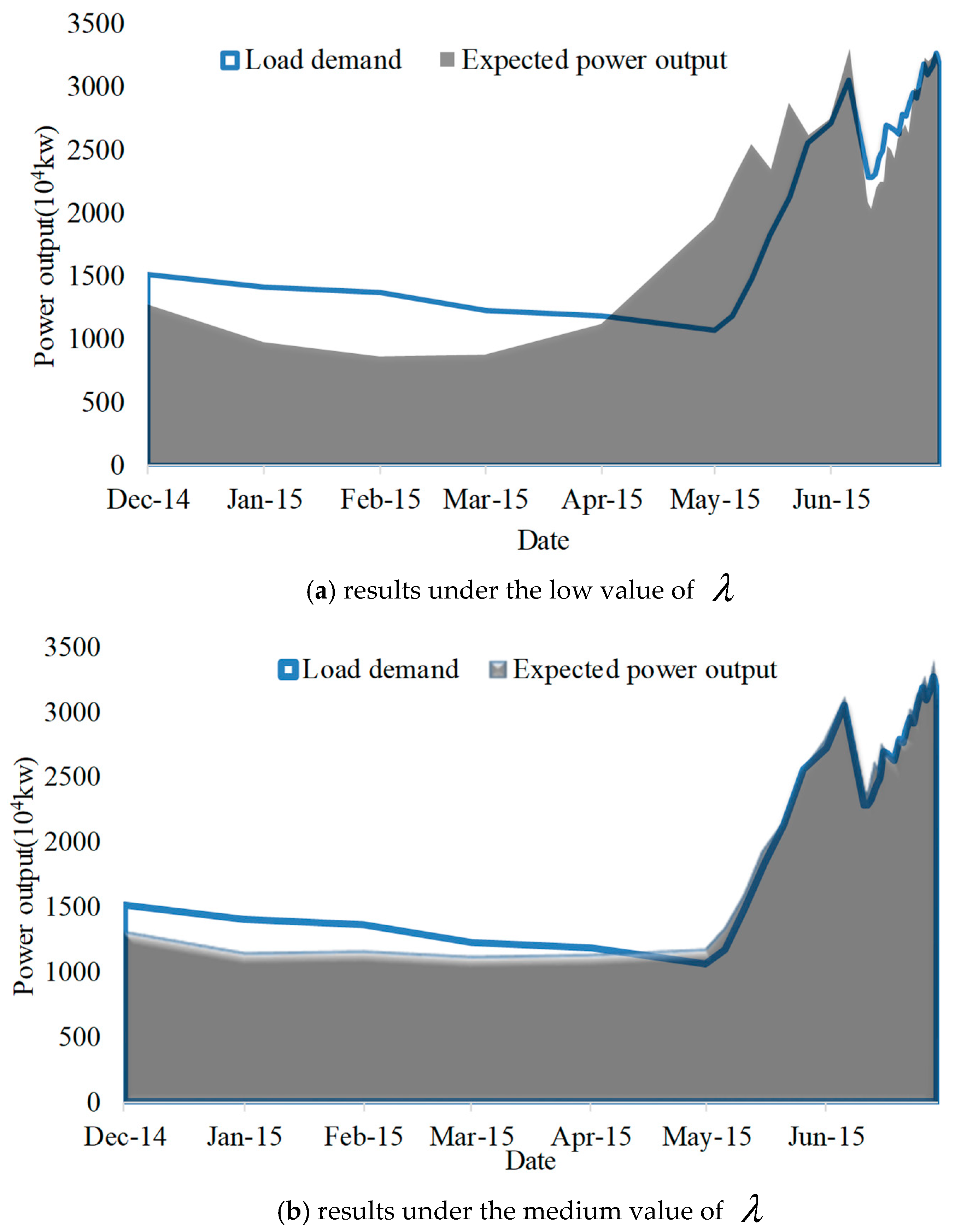
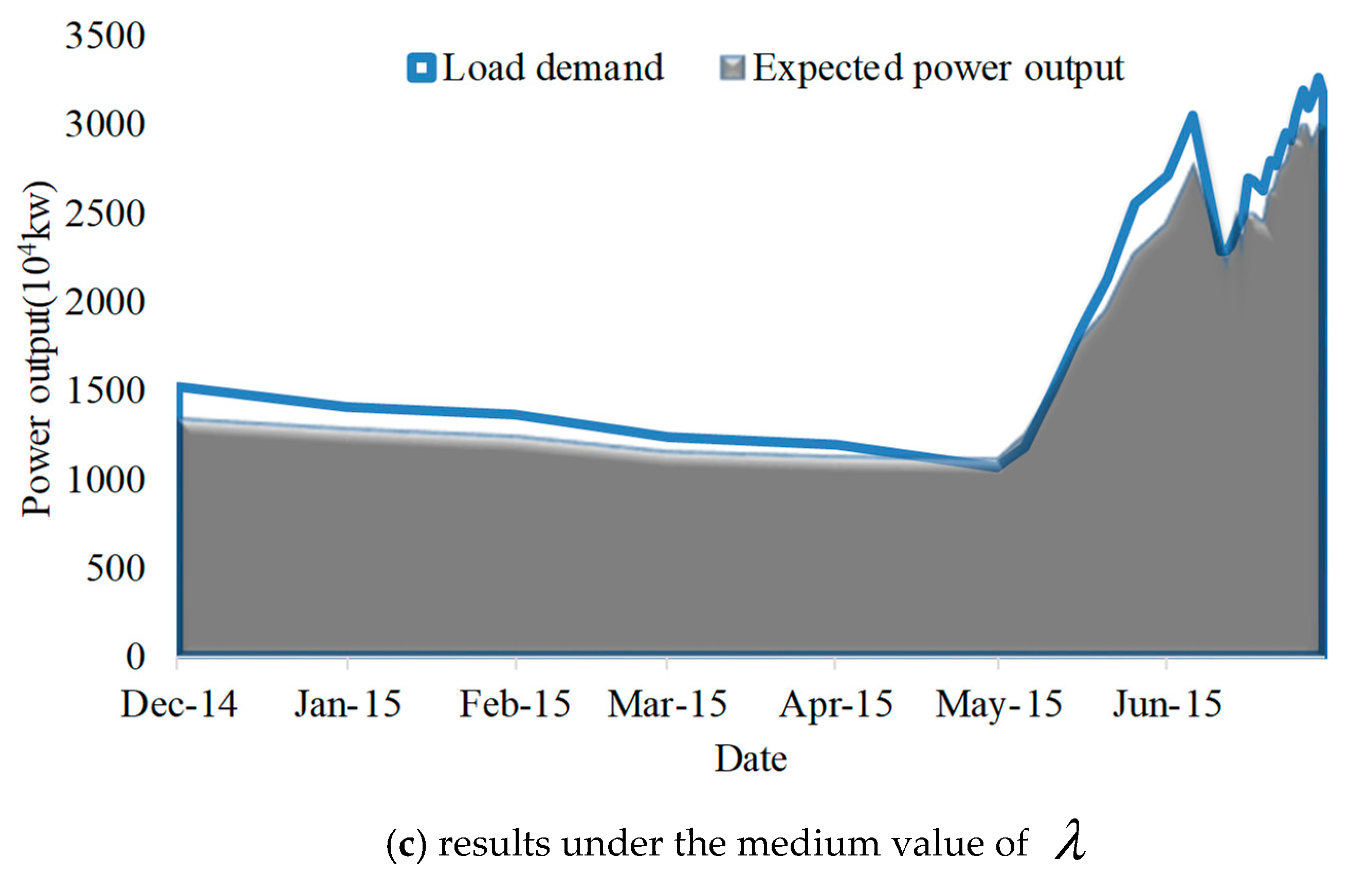
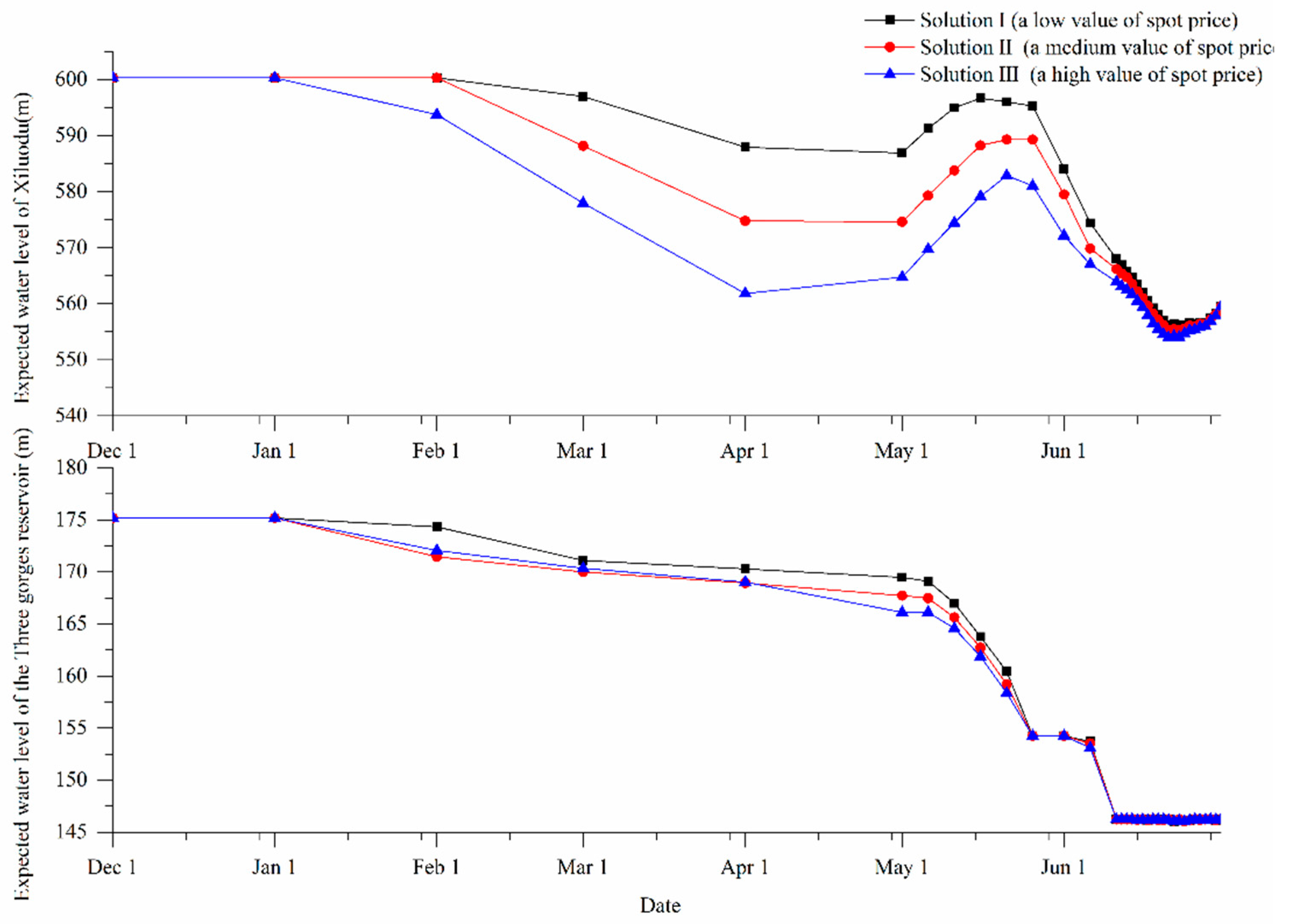
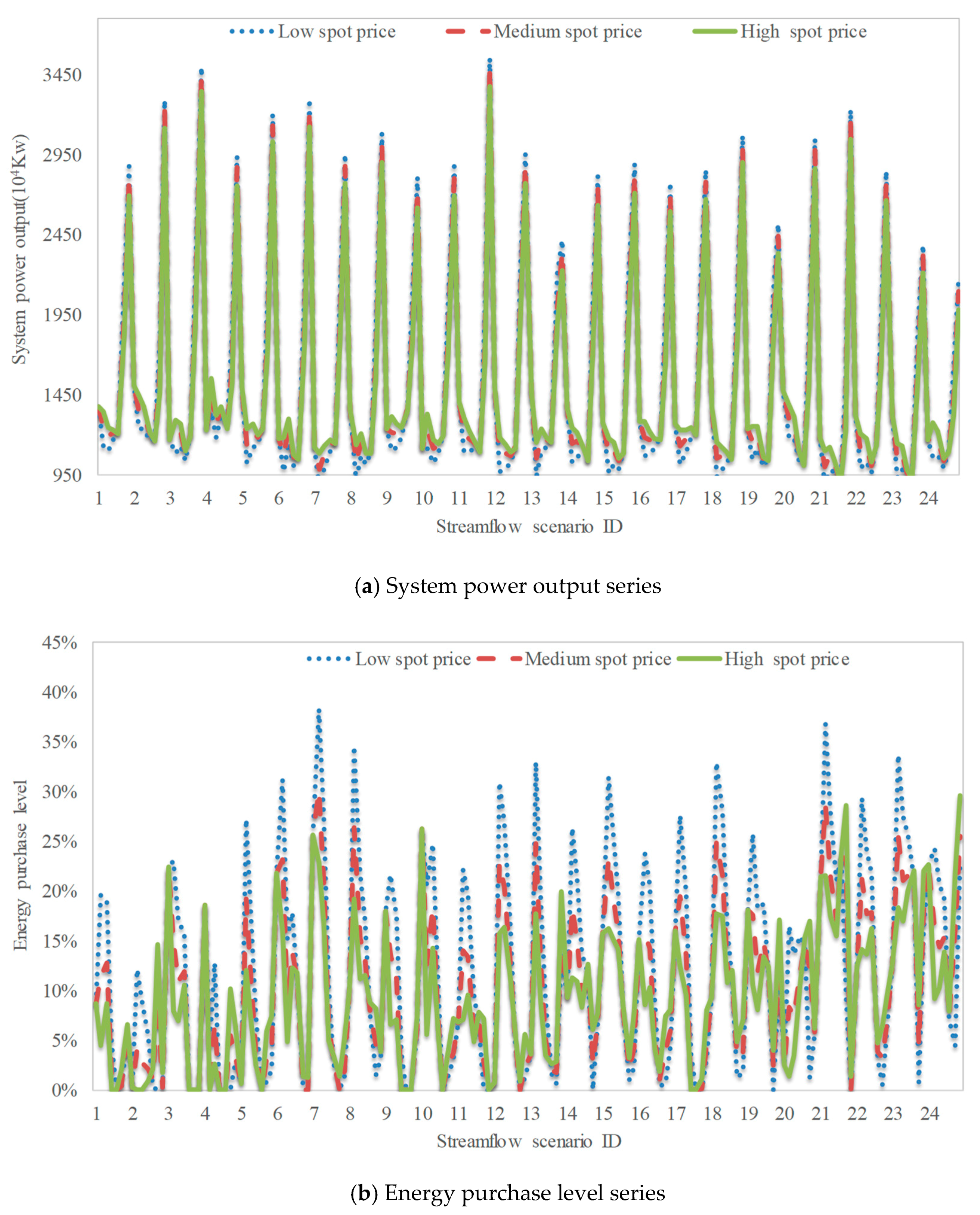
4.1. Tradeoffs under Streamflow Uncertainty

Table 2. Model parameters.

Reservoirs $(\mathit{m}=1,\dots ,4$)	${\mathit{V}}_{\mathit{m},1}^{}$ (108 m3)	${\mathit{V}}_{\mathit{m},\mathit{T}+1}^{}$ (108 m3)	$\overline{{\mathit{V}}_{\mathit{m},\mathit{t}+1}^{}}$ (108 m3)	$\underset{\_}{{\mathit{V}}_{\mathit{m},\mathit{t}+1}^{}}$ (108 m3)	$\underset{\_}{{\mathit{P}}_{\mathit{m},\mathit{t}}^{}}$ (104 kW)	$\overline{{\mathit{P}}_{\mathit{m},\mathit{t}}^{}}$ (104 kW)	$\mathit{p}$ (CNY/kWh)	$\mathsf{\Delta }\mathit{W}{\mathit{L}}_{\mathit{m}}$ (m/day)	$\mathit{\lambda }$ (CNY/kWh)	$\mathit{D}$ (108 kWh)
Xiluodu	115.72	69.23	115.72	51.12	120	1260	0.28	2	0.317, 0.356, 0.48 a	818.29
Xiangjiaba	49.767	40.74	49.767	40.73	82	600		1
Three Gorges	393.05	178.96	393.05	171.5	166	2250		0.6
Gezhouba	7.1	7.1	7.1	6.25	25	295		3

^a. The three values of $\lambda$ represent the low level, medium level and high level discretized scenario of spot energy price of energy purchase, respectively.

lists the model parameters. Three different levels of forecasted spot prices, $\lambda$, are tested to examine the influence of parameter variations on the outcome.

For each group of parameters, the deterministic equivalents are solved by a nonlinear solver, LINGO (https://www.lindo.com/). The robustness of model with varied constraint conditions of downstream water requirements and dynamic control on flood limited water levels has been verified by Xu et al. [31].

Figure 2 shows the box plots for the system revenue from energy production and energy purchase level under different values of $\lambda$. The expected system revenue and the expected energy purchase level decrease as $\lambda$ increases, which shows that the increase in expected total revenue adversely affects the minimization of expected energy shortfall percentage and vice versa. This finding is attributed to the fact that the contracted energy is satisfied by the energy production from this hydropower producer and energy purchase from other producers. As the expected energy purchase level decreases from 16.2% (under a low $\lambda$) to 12.3% (under a high $\lambda$), the expected system revenue decreases from 218.78 × 10⁸ CNY to 215.92 × 10⁸ CNY. Theoretically, this finding is attributed to the increase in $\lambda$, which enhances the cost of energy purchase, thereby leading to the decrease in energy shortfall for lowering the cost. Operation policy becomes more conservative for lowering down the expected energy shortfall percentage and deteriorates energy production.

This finding also shows that the variations in system revenue in terms of streamflow variability are nearly the same under different values of $\lambda$, whereas the variations in energy purchase level reduce gradually as $\lambda$ increases. This finding indicates that the variations in $\lambda$ has a more direct effect on the results of energy purchase level than the system revenue.

Figure 3 and Figure 4 show the optimal expected system power output sequences and expected water level trajectories under different values of $\lambda$, respectively. Under a low level of $\lambda$, the optimal solution (solution I) pursues the highest expected revenue, but it results in the highest level of energy purchase compared with the other two solutions under different scenarios of $\lambda$. Figure 3a shows that this solution results in the highest expected energy purchase level of 26.2% in January, but it generates a high level of energy surplus in May and June. As $\lambda$ gradually enhances, the highest expected energy purchase levels in a single period will decrease to 18.2% and 13.3%, respectively, whereas energy surplus in the late periods will decrease. The results show that lowering the down energy purchase causes the energy delivery policy to homogenize the energy shortfall results as $\lambda$ increases.

Figure 4 also indicates that the variations in energy delivery policy are due to the different reservoir drawdown policies. The Xiluodu and the Three Gorges project deplete their storages more rapidly as $\lambda$ increases. This finding explains the differences in energy delivery processes. To reduce the energy purchase in the early stage of the drawdown season when streamflow is low, reservoirs should fasten their storage depletions to increase production. Consequently, reservoirs could lose water head in the late stage such that the energy production in the late stage is reduced. The average water head of Xiluodu would decrease from 212.63 m to 200.84 m, whereas the average water head of the Three Gorges project would reduce from 101.4 m to 100.3 m. Given that the water head of both storage reservoirs are significantly reduced, the total energy production and the system revenue from energy production are reduced.

The risk-neutral results are obtained using the expected value of indices to measure the model’s mean performance. The outcome under each specific streamflow scenario may be different, thereby providing additional information about the distribution of indices.

Figure 5 plots the system power output and energy purchase levels under different streamflow scenarios and $\lambda$. Figure 5a shows that the expected value of the system power output and the variance of the system power output are reduced with the increase of $\lambda$. The reduction in variance is induced by the homogenization in energy delivery, which is validated as the cause of deteriorations in the expected value of system revenue due to the water head reduction. Figure 5b shows that the standard deviation of energy purchase level decreases from 10.3% to 7.08% as $\lambda$ increases. This finding indicates that the highest level of energy purchase was effectively reduced in most streamflow scenarios. However, few exceptions still exist. In the driest streamflow scenario, namely, Scenario 24, the highest energy shortage purchase under the case of a high $\lambda$ is 29.6%, which is even greater than the corresponding results under the medium and low value scenario of $\lambda$. This result is attributed to the reduction in expected value of an index in several scenarios, which does not necessarily guarantee its reduction under each scenario.

4.2. Net Revenue Results

The revenue from energy production and cost of energy purchase can be determined once the monetary value of energy purchase can be quantified using spot price $\lambda$. As discussed by Wang et al. [32], $\lambda$ also represents the decision makers’ risk preference toward uncertain real-time markets besides the economic interpretation. The sensitivity tests on the influence of $\lambda$ on the model results are essential for informed decision-making when forecasting $\lambda$ becomes difficult for either economic reasons or risk preference reasons.

Two extreme cases can be applied to determine the bounds of $\lambda$. If the power system is equipped with abundant and cheap power producers such that the energy shortfall can be easily mitigated, $(\lambda -p)$ tend to be zero. The objective characterized by Equation (6) is equivalent to the energy production maximization. This scenario could occur when the energy shortfall caused by inadequate energy delivery from this hydropower producer can be substituted by other similar hydropower producers. By contrast, $(\lambda -p)$ could also be as high as the price difference between the most expensive power source, such as thermal power source and nuclear energy source.

Table 3. Optimal model results under different values of $\lambda$ .

Expected Revenue from Energy Production $\mathbf{E}[\mathit{E}(\mathit{\omega },\mathit{\xi })]\cdot \mathit{p}$ (108 CNY)	Expected Energy Purchase Level (%)	Spot energy Price $\mathit{\lambda }$ (CNY/kWh)	Expected Cost of Energy Purchase $\mathbf{E}[\mathit{E}\mathit{s}(\mathit{\omega },\mathit{\xi })]\cdot (\mathit{\lambda }-\mathit{p})$(108 CNY)	Expected Net Revenue $\mathit{N}$ (108 CNY)
220.21	21.97	0.28	0	220.21
219.49	18.56	0.306	3.89	215.60
218.78	16.22	0.317	4.96	213.82
218.06	14.56	0.332	6.25	211.82
217.35	13.42	0.357	8.41	208.94
216.64	12.72	0.405	13.02	203.62
215.92	12.28	0.48	20.06	195.87

lists the optimal results of indicators under different values of $\lambda$ and Figure 6 plots the corresponding results.

The expected revenue from the energy production decreases from 220.21 × 10⁸ CNY to 215.92 × 10⁸ CNY with the reduced magnitude of 4.29 × 10⁸ CNY as $\lambda$ grows. By contrast, the expected cost of the energy purchase increases drastically from 0 to 20.06 × 10⁸ CNY, thereby showing that the influence of $\lambda$ on the expected cost dominates the influence on expected revenue. Therefore, the curve of the expected net revenue, as shown in Figure 6, reduces rapidly due to the increase in expected cost when $\lambda$ varies. The energy purchase becomes increasingly valuable when $\lambda$ is high.

The optimal solutions in determining the best level of energy purchase should be made according to the specific value of $\lambda$. However, when the prediction of $\lambda$ is not precise, decision makers are also concerned about the consequence, especially the worst consequence, if a non-optimal or sub-optimal decision is executed.

Figure 7 plots the results of net benefit under different levels of $\lambda$ and energy shortage percentages.

Thus, the following results are obtained:

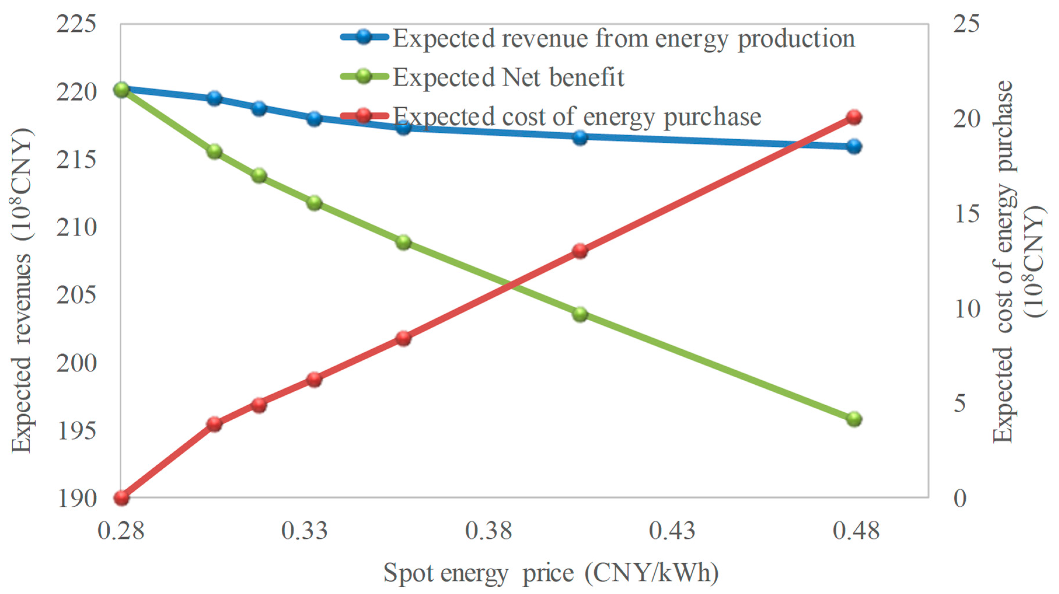
• From the horizontal view, the results of the net revenue under different levels of energy purchase level show that the difference between the highest net revenue and the lowest net revenue from each curve varies greatly with the specific level of $\lambda$. The difference is the cost of making the worst decision. For example, when the actual value of $\lambda$ is low ($\lambda =0.31$ CNY/kWh), but decision makers overestimate the value of $\lambda$ such that a most conservative decision ($E[S(\omega ,\xi )]=12.28\%$) on energy purchase level is made, the reservoirs system would lose a net revenue of 1.65 × 10⁸ CNY compared with the results given a perfect information on $\lambda$. The corresponding highest reduction in net revenue would be 11.52 × 10⁸ CNY when the actual value of $\lambda$ is extremely high ($\lambda =0.48$ CNY/kWh), but decision makers underestimate $\lambda$ and make a most progressive decision ($E[S(\omega ,\xi )]=21.97\%$). For the medium level of $\lambda$($\lambda =0.36$ CNY/kWh), the highest reduction in net revenue would be 2.5 × 10⁸ CNY. Therefore, if an inaccurate information on $\lambda$ is used, the loss in net revenue would be high, especially when $\lambda$ is high.
• From the vertical view, when the results of net revenue under different levels of $\lambda$ but the same level of energy purchase level, the deviated magnitude of the net revenue between the results of $\lambda =0.28$ and $\lambda =0.48$ would increase with the energy purchase level. This finding could be applied to decision-making when no reliable predicted information on $\lambda$ can be used. For example, if all the scenarios of $\lambda$ are assumed equally likely to occur, the expectation of net revenue under all possible $\lambda$ scenarios can be used as the target. Consequently, the optimal level of energy purchase would be 14.56% and the corresponding expected value of net revenue would be 209.27 × 10⁸ CNY. Therefore, medium-level energy purchase rather than a high-level or low-level energy purchase should be determined to balance revenue and cost if no predicted information of $\lambda$ can be used.

5. Discussion

For highlighting the differences of model performances, the model results are compared with two traditional models with the objective of maximizing the total energy production (or revenue of energy production) and the objective of minimizing the energy shortfall (or cost of energy purchase) under a high value scenario of $\lambda =0.41$ CNY/kWh.

Table 4. Statistics of results from different models under a high value of $\lambda$ .

Models	Expected Revenue from Energy Production (108 CNY)	Expected Cost of Energy Purchase (108 CNY)	Expected Net Revenue (108 CNY)
Energy production maximization	220.21	5.11	215.10
Energy shortfall minimization	214.49	1.51	212.98
Net revenue maximization	217.35	1.91	215.45

lists the model results while Figure 8 plots the power output shortfall or surplus related to the load demand.

The results show that the model with the single objective of maximizing revenue or minimizing cost does not yield an optimized net revenue for neglecting their tradeoffs. Instead, the proposed model could address the results tradeoffs under a deregulated market environment, which balances the energy production and energy purchase levels according to the specific conditions of inflow and price uncertainty. To maximize the total energy production could cause the highest level of energy purchase in early time periods, due to the nonlinear tradeoff mechanism of power generation over different time periods. To contrast, to minimize the energy shortfall (purchase) could lower down the total energy production, resulting in a reduction in direct revenue. The optimal policy for optimizing the net revenue seeks the best compromise of benefit and cost from the tradeoffs.

6. Conclusions

Hydropower producers under a deregulated electricity market could accomplish the long-term contracting of energy through the flexible choices of energy production delivery or energy purchase from other power producers in a real-time market. The energy production delivery associated with streamflow conditions varies and the cost of energy purchase is determined by spot energy price. Thus, the decisions of hydropower producers should be rationalized by benefit-cost analysis by considering the variations of streamflow and spot energy price. This study proposes a stochastic programming model to address the conflicting decisions under uncertain streamflow and spot energy price conditions. Conflicting objectives are resolved by maximizing the expected value of net revenue that jointly considers the revenue from energy production and the cost from energy purchase for possible shortfalls over all streamflow scenarios. The objective tradeoffs and conflicts resolutions are analyzed under different forecasted spot energy price conditions using sensitivity tests. The developed model framework is able to deal with uncertain decision making with uncertainties expressed by probability distributions and discretized scenarios. Methodologies are applied to guide the operations of the Three Gorges cascade reservoir system during the drawdown season. The results are as follows:

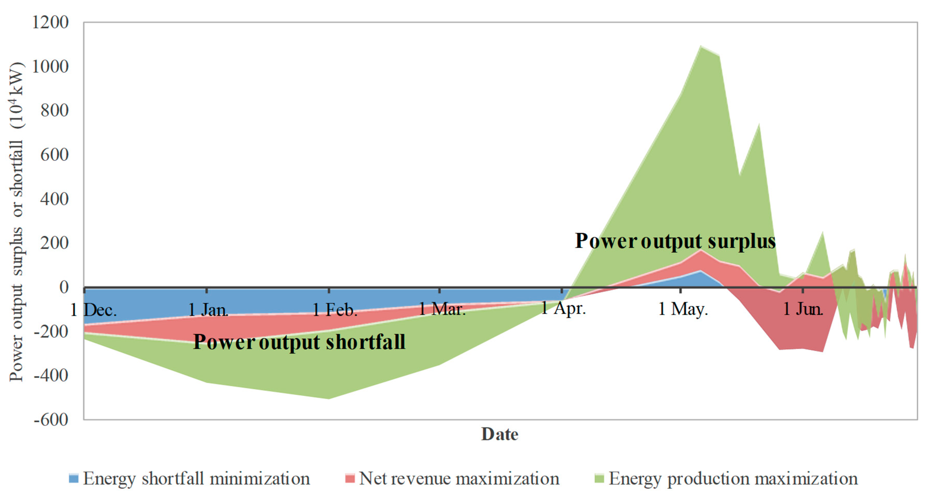
• An increase in expected total revenue adversely affects the reduction of expected energy shortfall percentage or energy purchase level because the mechanism of maximizing the hydropower generation could deviate from the mechanism of minimizing the energy purchase level over sequences of periods. In this case study, maximizing the hydropower generation yields a postponed drawdown policy for increasing water head. This finding generates heterogeneous energy production that intensifies the energy purchase level.
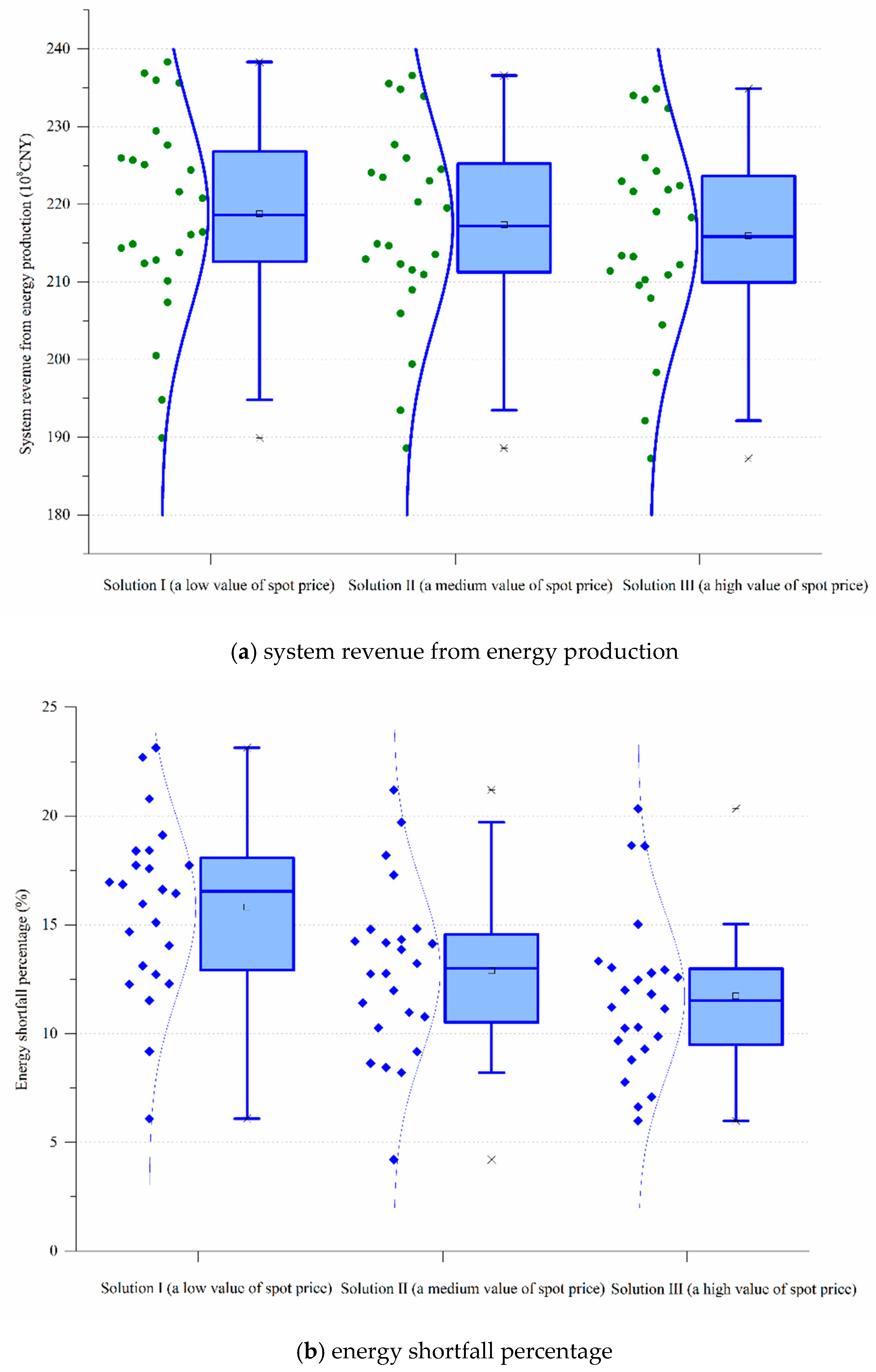
• An increase in spot energy price decreases the expected energy production and energy purchase level because of its direct influence on the drawdown operation policy and the cost of energy purchase. However, this phenomenon does not apply to all streamflow scenarios.
• A precise forecast on the spot energy price provides valuable information regarding its influence on the net revenue. By contrast, sustaining a medium-level energy purchase could outperform the choices of a high-low-level energy purchase in terms of expected value of net revenue over different price scenarios if no accurate predicted information on the spot energy price can be obtained.
• The nonlinear tradeoff results of energy surplus and energy shortfall provide valuable information for determining the compromise of benefit and cost, and the model could yield the optimal policy considering both terms and the influences of inflow and price uncertainties.

For assisting real-time hydropower operations, frequently updated information of forecasted streamflows and penalizing prices information should be employed when using the methodologies. The discretized price scenario information primarily facilitates the decision of the optimal range of energy purchase level, energy production level as well as optimal drawdown policies. The proposed methodologies mainly suite for the situation under which the price uncertainty cannot be precisely expressed by probability distributions. Accordingly, optimal decisions are associated with finite predicted price scenarios and the controls on releases and water levels are primarily on fuzzy or inexact ranges. Based on the proposed model framework, further studies could explore the use of specified distributions on spot price and the correlations with streamflow uncertainty when the information is available, this could drive a complex model which considers multiple uncertain sources and their mutual influences. Moreover, for dealing with multiple uncertainties, numerical model reduction techniques have to be investigated for ensuring affordable computational effort. With more relevant information considered, it is expected that more accurate and stable decisions can be determined.

References

1. Chang, X.; Liu, X.; Zhou, W. Hydropower in China at present and its further development. Energy 2010, 35, 4400–4406. [Google Scholar] [CrossRef]
2. World Energy Council. World Energy Resources Hydropower|2016; World Energy Council: London, UK, 2016; pp. 1–53. [Google Scholar]
3. Xu, B.; Boyce, S.E.; Zhang, Y.; Liu, Q.; Guo, L.; Zhong, P. Stochastic programming with a joint chance constraint model for reservoir refill operation considering flood risk. J. Water Resour. Plan. Manag. 2017, 143, 4016067. [Google Scholar] [CrossRef]
4. Xu, B.; Zhong, P.; Stanko, Z.; Zhao, Y.; Yeh, W.W.G. A multiobjective short-term optimal operation model for a cascade system of reservoirs considering the impact on long-term energy production. Water Resour. Res. 2015, 51, 3353–3369. [Google Scholar] [CrossRef] [Green Version]
5. Xu, B.; Zhong, P.; Wan, X.; Zhang, W.; Chen, X. Dynamic feasible region genetic algorithm for optimal operation of a multi-reservoir system. Energies 2012, 5, 2894–2910. [Google Scholar] [CrossRef]
6. Feng, Z.; Niu, W.; Cheng, C.; Wu, X. Optimization of hydropower system operation by uniform dynamic programming for dimensionality reduction. Energy 2017, 134, 718–730. [Google Scholar] [CrossRef]
7. Zhao, T.; Zhao, J.; Liu, P.; Lei, X. Evaluating the marginal utility principle for long-term hydropower scheduling. Energy Convers. Manag. 2015, 106, 213–223. [Google Scholar] [CrossRef]
8. Xu, B.; Zhong, P.; Zhao, Y.; Zhu, Y.; Zhang, G. Comparison between dynamic programming and genetic algorithm for hydro unit economic load dispatch. Water Sci. Eng. 2014, 7, 420–432. [Google Scholar]
9. Li, X.; Li, T.J.; Wei, J.H.; Wang, G.Q.; Yeh, W.W. Hydro unit commitment via mixed integer linear programming: A case study of the Three Gorges project, China. IEEE Trans. Power Syst. 2014, 29, 1232–1241. [Google Scholar] [CrossRef]
10. Li, J.Q.; Marino, M.A.; Ji, C.M.; Zhang, Y.S. Mathematical models of inter-plant economical operation of a cascade hydropower system in electricity market. Water Resour. Manag. 2009, 23, 2003–2013. [Google Scholar] [CrossRef]
11. Kern, J.D.; Characklis, G.W.; Doyle, M.W.; Blumsack, S.; Whisnant, R.B. Influence of deregulated electricity markets on hydropower generation and downstream flow regime. J. Water Resour. Plan. Manag. 2012, 138, 342–355. [Google Scholar] [CrossRef]
12. Wolfgang, O.; Haugstad, A.; Mo, B.; Gjelsvik, A.; Wangensteen, I.; Doorman, G. Hydro reservoir handling in Norway before and after deregulation. Energy 2009, 34, 1642–1651. [Google Scholar] [CrossRef]
13. Liu, H.L.; Jiang, C.W.; Zhang, Y. A review on risk-constrained hydropower scheduling in deregulated power market. Renew. Sustain. Energy Rev. 2008, 12, 1465–1475. [Google Scholar]
14. Zhong, P.A.; Zhang, W.; Xu, B. A risk decision model of the contract generation for hydropower generation companies in electricity markets. Electr. Power Syst. Res. 2013, 95, 90–98. [Google Scholar] [CrossRef]
15. Mo, B.; Gjelsvik, A.; Grundt, A. Integrated risk management of hydro power scheduling and contract management. IEEE Trans. Power Syst. 2001, 16, 216–221. [Google Scholar] [CrossRef]
16. Birge, J.R.; Louveaux, F. Introduction to Stochastic Programming; Springer Science & Business Media: New York, NY, USA, 2011; p. 485. [Google Scholar]
17. Xu, B.; Zhong, P.A.; Zambon, R.C.; Zhao, Y.; Yeh, W.W.G. Scenario tree reduction in stochastic programming with recourse for hydropower operations. Water Resour. Res. 2015, 51, 6359–6380. [Google Scholar] [CrossRef] [Green Version]
18. Latorre, J.M.; Cerisola, S.; Ramos, A. Clustering algorithms for scenario tree generation: Application to natural hydro inflows. Eur. J. Oper. Res. 2007, 181, 1339–1353. [Google Scholar] [CrossRef]
19. Côté, P.; Leconte, R. Comparison of stochastic optimization algorithms for hydropower reservoir operation with ensemble streamflow prediction. J. Water Res. Plan. Manag. 2015, 2, 04015046. [Google Scholar] [CrossRef]
20. Tilmant, A.; Kelman, R. A stochastic approach to analyze trade-offs and risks associated with large-scale water resources systems. Water Resour. Res. 2007, 43, W064256. [Google Scholar] [CrossRef]
21. Kelman, J.; Stedinger, J.R.; Cooper, L.A.; Hsu, E.; Yuan, S.Q. Sampling stochastic dynamic-programming applied to reservoir operation. Water Resour. Res. 1990, 26, 447–454. [Google Scholar] [CrossRef]
22. Li, Y.P.; Huang, G.H.; Chen, X. Multistage scenario-based interval-stochastic programming for planning water resources allocation. Stoch. Environ. Res. Risk Assess. 2009, 23, 781–792. [Google Scholar] [CrossRef]
23. Si, Y.; Li, X.; Yin, D.; Liu, R.; Wei, J.; Huang, Y.; Li, T.; Liu, J.; Gu, S.; Wang, G. Evaluating and optimizing the operation of the hydropower system in the Upper Yellow River: A general LINGO-based integrated framework. PLoS ONE 2018, 13, e191483. [Google Scholar] [CrossRef] [PubMed]
24. Li, F.; Qiu, J. Multi-objective reservoir optimization balancing energy generation and firm power. Energies 2015, 8, 6962–6976. [Google Scholar] [CrossRef]
25. You, J.; Cai, X. Hedging rule for reservoir operations: 1. A theoretical analysis. Water Resour. Res. 2008, 44, 1–9. [Google Scholar] [CrossRef]
26. Draper, A.J.; Lund, J.R. Optimal hedging and carryover storage value. J. Water Resour. Plan. Manag. 2004, 130, 83–87. [Google Scholar] [CrossRef]
27. Xu, B.; Zhong, P.; Huang, Q.; Wang, J.; Yu, Z.; Zhang, J. Optimal hedging rules for water supply reservoir operations under forecast uncertainty and conditional value-at-risk criterion. Water 2017, 9, 568. [Google Scholar] [CrossRef]
28. Chen, F.; Liu, B.; Cheng, C.; Mirchi, A. Simulation and regulation of market operation in hydro-dominated environment: The Yunnan case. Water 2017, 9, 623. [Google Scholar] [CrossRef]
29. Dhaubanjar, S.; Davidsen, C.; Bauer-Gottwein, P. Multi-objective optimization for analysis of changing trade-offs in the Nepalese water-energy-food nexus with hydropower development. Water 2017, 9, 162. [Google Scholar] [CrossRef]
30. Shamshad, A.; Bawadi, M.; Wanhussin, W.; Majid, T.; Sanusi, S. First and second order Markov chain models for synthetic generation of wind speed time series. Energy 2005, 30, 693–708. [Google Scholar] [CrossRef]
31. Xu, B.; Zhong, P.; Chen, Y.; Zhao, Y. The multi-objective and joint operation of Xiluodu cascade and Three Gorges cascade reservoirs system. Sci. Sin. Technol. 2017, 47, 823–831. (In Chinese) [Google Scholar]
32. Wang, Y.Y.; Huang, G.H.; Wang, S. CVaR-based factorial stochastic optimization of water resources systems with correlated uncertainties. Stoch. Environ. Res. Risk Assess. 2016, 31, 1543–1553. [Google Scholar] [CrossRef]
Figure 1. Location sketch map of the Three Gorges cascade reservoir system.
Water 10 00885 g001
Figure 2. Optimal model results under different values of spot energy price.
Water 10 00885 g002
Figure 3. Load demand and expected power output trajectories under different values of λ .
Water 10 00885 g003aWater 10 00885 g003b
Figure 4. Expected variations in water levels of Xiluodu and the Three gorges reservoir.
Water 10 00885 g004
Figure 5. System power output and energy purchase level results under different streamflow scenarios and λ
Water 10 00885 g005
Figure 6. Revenue, cost, and net revenue under different spot energy prices.
Water 10 00885 g006
Figure 7. Net revenue results under different values of λ and energy purchase levels.
Water 10 00885 g007
Figure 8. Power output shortfall and surplus trajectories under different models.
Water 10 00885 g008