Streamflow Simulation Using Bayesian Regression with Multivariate Linear Spline to Estimate Future Changes


1
Department of Civil and Environmental Engineering, The Hong Kong University of Science and Technology, Clear Water Bay, Kowloon, Hong Kong, China
2
Institute of Engineering Research, Seoul National University, Seoul 08826, Korea
3
Walmart Labs, Salarpuria Touchstone, Outer Ring Rd, Bengaluru, Karnataka 560103, India
*
Author to whom correspondence should be addressed.
Water 2018, 10(7), 875; https://doi.org/10.3390/w10070875
Submission received: 1 June 2018
/
Revised: 23 June 2018
/
Accepted: 28 June 2018
/
Published: 30 June 2018
(This article belongs to the Section Hydrology)
Abstract
:Statistical models for hydrologic simulation are a common choice among researchers particularly when catchment information is limited. In this study, we adopt a new statistical approach, namely Bayesian regression with multivariate linear spline (BMLS) for long-term simulation of streamflow on a Hydroclimate Data Network (HCDN) site in the United States. The study aims to: (i) evaluate the performance of the BMLS model; (ii) compare the performance of climate model outputs as predictors in hydrologic simulation; and (iii) estimate the changes in streamflow caused by anthropogenic climate change which is defined as the projected change in precipitation and temperature under different greenhouse gas emission scenarios. Performance of the BMLS model is compared with climatology for the validation period. Results suggest that the BMLS model forced with observed monthly precipitation and average temperature exhibits information that is not presented in the climatology of the validation period. Later, we consider Coupled Model Intercomparison Project Phase 5 (CMIP5) historical and hindcast runs to simulate streamflow at the HCDN site. The study found that sea-surface temperature-initialized decadal hindcast runs are performing no better than 20th century historical runs regarding hydrologic simulation. Finally, the changes in mean and variability in streamflow at the HCDN site are estimated by forcing the model with CMIP5 future projections for the period 2000–2049.
1. Introduction
Simulation of monthly streamflow serves various purposes of water resources planning and management. Decadal simulation of streamflow provides years-ahead insight on the capacity, adequacy, and reliability of a reservoir based on the anthropogenic changes in runoff [1,2,3]. Conceptual and physically based models of the watershed, for example, SWAT (Soil and Water Assessment Tool), VIC (Variable Infiltration Capacity Macroscale Hydrologic Model), and PIHM (Penn State Integrated Hydrologic Modeling System) remain a popular choice among water resources managers. Such a model has the potential to include every component of a hydrologic process (conceptual) or mathematically replicate the physical phenomenon. A review of few physically-based models is provided by Devi et al. [4]. These models require a bunch of data sets that delineate hydro-geological characteristic of a basin.
Statistical and machine learning techniques for rainfall-runoff modeling, also known as empirical modeling, have received significant attention from the researchers particularly in cases where supporting input data for process-based models are limited [5]. Further improvement and application of statistical and machine learning techniques remain popular among researchers, despite the fact that these models are often criticized as black box models [6], ignoring the physical process. A simple rainfall-runoff model considers precipitation as the model input and days to the years-ahead prediction of the streamflow as the model output. Empirical approaches for streamflow simulation may vary from simple regression to sophisticated machine learning algorithms such as an artificial neural network (ANN). Sharma et al. [7] proposed a method to generate synthetic streamflow sequences based on kernel estimates of the joint and conditional probability density. The study produces sequences that represent future scenarios assuming that future remains similar to the past. Random number generator was used by Hirsch [8] to simulate the traces of normally distributed innovations. Following that, studies [9,10,11] employed several random sampling algorithms for uncertainty analysis and comparison purposes of network design [1]. Recent studies focused on developing copula-based methods for monthly streamflow simulations [12,13]. Shortridge et al. [14] compared a machine learning algorithm with a statistical approach-multiple regression to simulate streamflow over five rivers of Ethiopia. On the machine learning side, support-vector machines [15,16], regression tree based approach [5,17], and ANN [18,19] were used for rainfall-runoff modeling.
The objective of the present study is to employ a state-of-the-art statistical approach, Bayesian regression with multivariate linear spline (BMLS), for decades-ahead monthly streamflow simulation. The approach, initially proposed by Holmes and Mullick [20], incorporates Bayesian analysis of the piece-wise linear model. The piece-wise linear model is formed with basis functions that generalize the univariate spline to higher dimensions [20]. BMLS builds a regression surface with spline bases which select the covariate interactions uniformly and make the orientations suitably in all possible directions so that the estimated model has joint posterior optimality. The posterior model space of randomly located splines is integrated to obtain the posterior distribution of the response variable, streamflow in our case. The model features enable a smooth mean regression surface (posterior) from non-smooth piecewise prior model space. BMLS could be advantageous over existing statistical approaches for streamflow modeling since BMLS can deal with a large number of covariates while eliminating the irrelevant ones. The approach is also considered to be spatially adaptive [20].
The current study estimates the changes in future streamflow caused by climate change using BMLS. The study also examines the quality of general circulation models’ (GCM) outputs in simulating streamflow. The Coupled Model Intercomparison Project Phase 5 (CMIP5) introduced hindcast runs, in addition to the historical runs, where climate models are driven by initialized sea-surface temperature (SST) [21]. Hindcast runs, also known as decadal predictions, provide climate simulations for 10 and/or 30 years. These runs are archived as decadal-80, decadal-90, etc. based on the year of SST initialization. Earlier studies found that hindcast runs have the potential of preserving the precipitation and temperature cross-correlation [22] and of predicting long-lead ENSO (El Niño-Southern Oscillation) events [23]. Current study forces BMLS with outputs from multiple hindcast and historical runs to understand the improvement in empirical streamflow simulation from the SST initialization.
2. Dataset
2.1. Observed Streamflow
The current study uses a stream-gauge station located at Nottoway River near the stony creek, VA (USGS Site No. 02045500). The station is archived in the Hydro-Climatic Data Network (HCDN) Basins by the United States Geological Services (USGS). USGS provides a list of more than 1600 such virgin basins, distributed over the country [24]. HCDN basins are least affected by human-induced activities such as dams, urban development, groundwater lifting or recharge. Several studies reported that the impact of climate change on water resources could be best accessed on virgin basins [25,26,27].
For modeling purposes, we have excluded the land-use and land-pattern data. We build our model using historic streamflow, precipitation and temperature data. We expect that streamflow can be mapped efficiently with these few types of predictors. The station selection was difficult since there are thousands of HCDN stations. We focused on the data availability over a sufficient period. Another criterion for station selection was that the station should be located at the south-east of the United States since the south-east has experienced extreme meteorological events over the last few decades. The basin has a contributory area of 577 sq. miles. Observed streamflow values (in cubic feet per seconds) for the period January 1951 to December 1999 are used. The gauge has a datum of 58.42 ft above NGVD29. Mean basin elevation is 370.0 ft above NGVD29. Whereas, the average channel slope is 5.3 ft/mile. The time resolution of the data is monthly.
2.2. Observed and General Circulation Model (GCM) Precipitation and Temperature
On the predictor side, we obtain observed monthly precipitation and monthly average temperature series [28] from the Bureau of Reclamation’s archive. The observed dataset is provided on rectangular grids with resolution (1.0° × 1.0°). We select eight grid points that make 16 predictors in total, covering an area slightly more than the contributory area. BMLS has the inherent ability to handle an additional set of predictors. The time span of the predictor dataset and time resolution is the same as the predictand. Precipitation has the unit of mm/day and temperature is in degree Celsius. We also obtain precipitation (pr) and average temperature (tas) values from 12 GCMs from the CMIP5 experiments [21] to force the model for the future period. Only three GCMs, CNRM-CM5, IPSL-CM5-LR, and MPI-ESM-LR, are used to compare the quality of hindcast and historical runs. These three GCMs were used by an earlier study to compare hindcast and historical runs in estimating the cross-correlation between precipitation and temperature [29]. GCM historical run outputs are obtained for two time-slices, 1981–1999 (model validation period) and 2000–2049 (future simulation period). Climate information from the historical runs is obtained for the period 1950–1999 (20th century control run) and later trimmed for the time slice 1981–1999. Whereas, hindcast run outputs from three GCMs are obtained for the model validation period only, i.e., 1981–1999. Precipitation and temperature values for hindcast runs of the model validation periods are extracted from the decadal-80 run. Details regarding the grid points, temporal resolution, etc. of the GCM outputs are the same as observed climate predictors. Details regarding the GCM dataset is provided in Table 1. The current study includes future projections for two emission scenarios RCP 4.5 and RCP 8.5. Future streamflow is estimated by pooling all members of a model ensemble. Readers who are interested in the experimental design of CMIP5 are requested to follow Taylor et al. [21].
2.3. Data Diagnosis
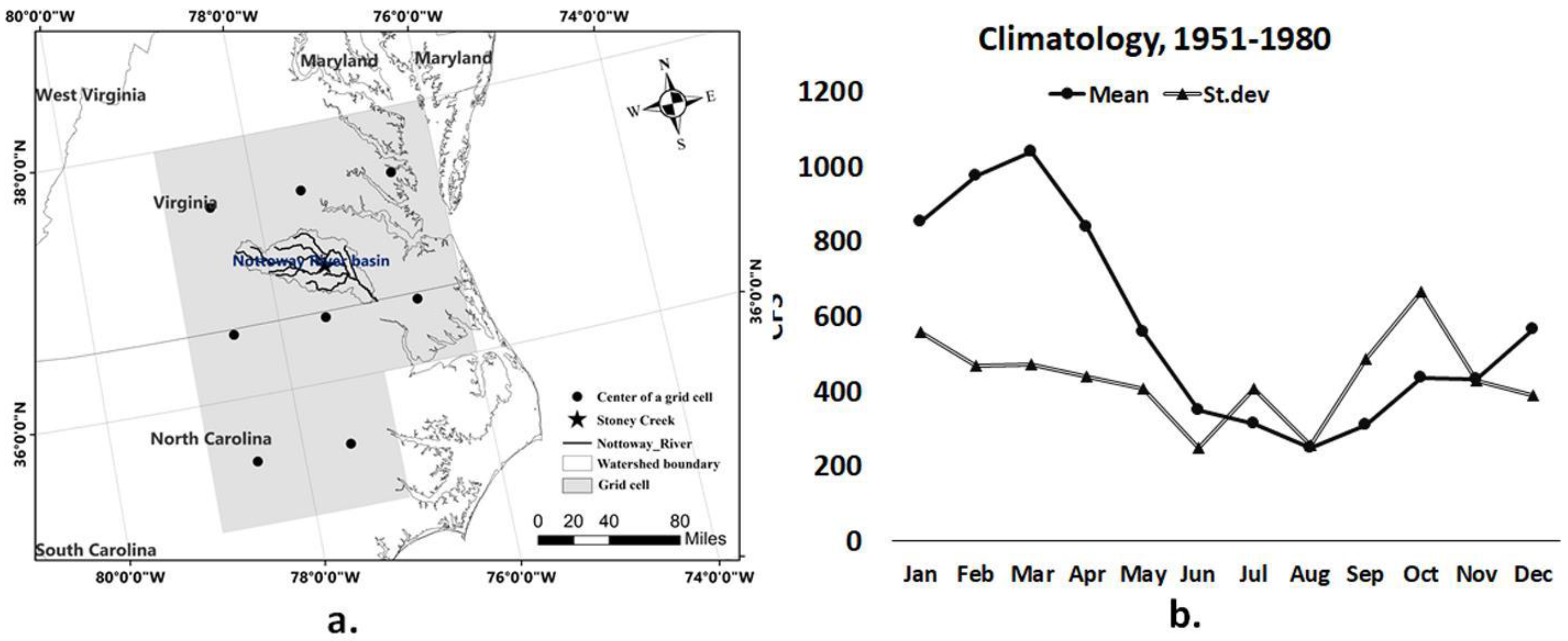
Information regarding the study area and climatology of streamflow during the calibration period are provided in Figure 1. The grids that encompass the region have the coordinates of [76.5–78.5°] E to [35.5–37.5°] N (Figure 1a). Figure 1b shows the long-term mean and standard deviation of monthly streamflow for the model training period (1951–1980). In Figure 1b we excluded the observation streamflow information for the period 1981–1999 since BMLS is forced with hindcast and historical run outputs for the period 1981–1999 (i.e., model validation period). High flow months are January, February, March, and April, indicating the high flows as a result of snowmelt or heavy winter precipitation. The region typically witnesses a humid subtropical climate. Low flows on the river occur during July, August, and September. The gauge station experiences almost the same amount of variance in monthly streamflow across the months. Standard deviation reaches a peak during October with values higher than 600 cfs, and the moment is lowest during June with values around 250 cfs.
3. Methodology
We use monthly temperature, precipitation and streamflow series obtained over a period of 360 months for the model-building purpose. The log-transformed streamflow is considered as the predictand. Let us denote St as the log-transformed streamflow, Ttk as the temperature and Ptk as the precipitation at the kth grid cell (k = 1, 2, …, 8) as observed on tth month (t = 1, 2, ..., 360).
There are eight variables on precipitation and eight variables on temperature. The proposed model is
The purpose of is to handle the temporal dependence of streamflow (defined as ). We assume has a known functional structure, for the current study, a seasonal autoregressive model (SAR) given by Φ, where Φ, where B is the lag operator, and s represents the period of the seasonal component. We incorporate the dependence of streamflow as a function of historical streamflow data of length h to ensure that the serial dependence of streamflow at lags of multiples of s are present as a source of variation. Here, s being the period of the seasonal components is necessarily the number of observations that make up a seasonal cycle. From the periodogram, autocorrelation and partial autocorrelation-based analysis, we choose a SAR model with s = 10, h = 3. The SAR model parameters are estimated using the maximum likelihood method which auto-detects the appropriate order of seasonal differencing. The estimated model is denoted by . Running the optimization on our data, we discovered s = 10 lag maximizes the overall joint likelihood. However, a lag of 12 months is typical in the case of monthly streamflow data. In fact, the choice of s = 12 would make the joint likelihood very close to the overall global optima which is reached at s = 10 in our case. Some hidden effects which we did not take into consideration in the current study, primarily attributed to additional covariates, might result in the value of the seasonal component. This could also be due to the fact that the time series component could have an unkonwn non-linear component. Nevertheless, we continue with the choice of s = 10, corresponding to the global optima.
Based on the estimated values of the function , the residuals are evaluated as . In the next stage, the main idea is to use the covariate information present in by {} and {} to explain the remaining variations present in to increase the goodness of fit of the overall model. We build a regression of the residuals obtained at the first stage, given by on the covariate information given by {} and {} by means of
We assume to be a smooth function with an unknown semi-parametric form. We perform a principal component-based variable selection and find that only first two principal components () of precipitation variables explain more than 90% variations due to {}. On the temperature side, the 1st principal component, denoted by explains more than 98% variation due to {}.
We reduce the model complexity of the prediction function given in Equation (1) by replacing it with a lower dimensional surrogate, denoted by (). Our study fits a regression of the residuals obtained using the SAR model at the first stage, given by on the covariate information by means of the regression function (.) by multivariate Bayesian Gaussian smoothing spline, discussed in the next section. Apart from a few modifications to serve the current problem, the method is primarily based on the work of Holmes and Mallick [20]. Combining the estimates obtained by the SAR model at the first stage and multivariate Bayesian Gaussian spline regression model of first stage residuals on the covariates, obtained at the second stage, our predictive model for time point t is defined as
3.1. Model Description
To understand the idea of the multivariate Bayesian Gaussian smoothing spline, let us consider a straightforward single predictor model given by Y = f(x) + ε, where a < x < b. Furthermore, x can be split into many small segments given by a = < … << < = b, the internal knots within the interval [a, b] being { and the two terminal points being and . A standard univariate spline involves fitting piecewise polynomial in each of the subintervals as for x where k = 1, …, (p + 1).
For the piecewise linear polynomial, the (p + 1) linear functions involving 2(p + 1) parameters, which under certain restriction(s) on continuity at the knots , can be reduced to (p + 2) independent parameters due to (p + 2) basis functions: (x), (x), … (x). The model to be fitted simply becomes, . The orthogonal basis functions for univariate linear spline are 1, x, where . Hence the model becomes, . The unknown parameters to be estimated are .
For linear univariate splines, the basis functions can be written as a dot product given by . The multivariate extension of this representation is considered for multidimensional covariates, say l (l > 1) component covariates. For multivariate spline, denoting and , the basis functions are analogously written as dot product given by
Note that, determines the position and denote the orientation of the basis plane in the dimensional covariate space. Hence, the multivariate spline smoother effectively becomes .
One modification is introduced in this model as a provision of variable selection by equating some of the elements of to 0. The modification makes the corresponding component of x vanish. Hence, the basis planes become perpendicular to some of the covariates. We define where = 1 if the dth element of is nonzero, else = 0. Furthermore, we define = as the number of non-zero elements in . The interpretation of is that it is effectively the number of interaction levels among covariates allowed in jth basis.
3.2. Prior Selection
In our case, p is the number of knots and z|p is the number of interaction levels, given there are p knots. Note that, ν is the vector of indicator variables, where the dth component of ν is indicating whether the dth element of ξ is 0. The following prior assumptions are made:
where Z is the maximum levels of interaction, which is fixed at 2 in our investigation. Holmes and Mallick [20] suggested the prior specifications to ensure that the orientation of the basis is uniformly distributed in the zth dimensional covariate space.
p ∼ Uniform(0, 1, 2, ..., ∞), z|p ∼ Uniform (1, 2, ..., Z),
(ν|z, p) ∼ Uniform on {(0, 1) × (0,1) × … × (0, 1)},
The regression parameters, α effectively are the position and gradient of the plane. Since a larger gradient leads to a rougher surface, regression parameters are centered at 0. The prior distribution of the parameters is given by
3.3. Posterior Computation
The data on the residuals obtained based on the SAR model and the covariates are denoted by D = {()}i=1,2,...,n. Posterior distribution of is
where, = VY V = , = + n/2, = + (1/2)(Y − V−1) and
The steps for posterior updating of ξ are as follows:
- Initialise the parameters to zero, = (0, …, 0).
- Draw from Zj ∼Uniform [I, …, Z] to fix the level of interactions among the covariates at the jth basis.
- To fix which covariates to be kept non zero, we select zj elements of νj at random and set the values to 1. Then we select the corresponding elements of and draw samples from a Gamma (1, 1) distribution. We normalize the elements of . Taking the square root of each element, we reverse the sign with probability 0.5.
- Select a data point at random and make .
- Finally, are simulated from the conditional distribution given in Equation (7).
Steps 1–3 ensure that the new plane is uniformly rotated in the zj selected dimension indicated by νj and perpendicular to all other covariates. Step 4 ensures that the boundary of the new plane passes through at least one data point.
Let us assume, an old set of simulated parameters as θ = (ξ, α, σ2, p, z, ν), and a new set of parameters as . The acceptance probability of a simulated sample is given in Holmes and Mallick [20] as
The acceptance ratio is a standard model choice criterion when a broad set of model parameters and hyperparameters are considered. The ratio also satisfies any concerns related to overfitting. The Markov Chain Monte Carlo (MCMC) algorithm is carried out using the ratio as the sample acceptance probability during the MCMC simulation from the posteriors. The MCMC simulation is repeated until we have enough number of samples to ensure the convergence of the chain to a stationary distribution. The average of the piecewise linear surfaces generated as a result of the MCMC simulation is accepted as the posterior estimate of the Bayesian multivariate linear spline from the joint posteriors of the parameters. The estimated model is further used to issue predictions, as described in the following section.
3.4. Experimental Design
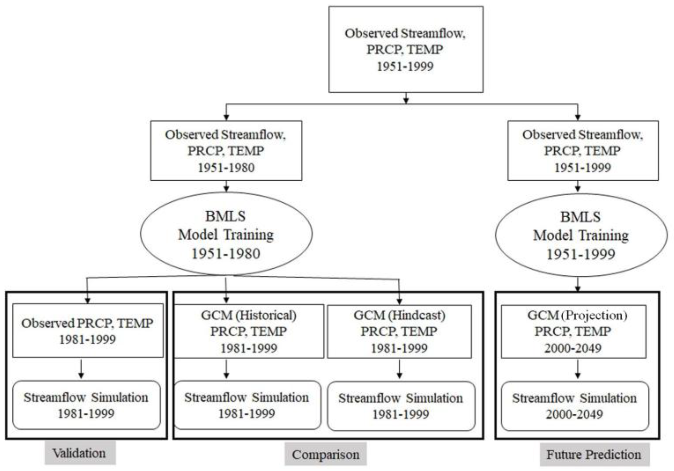
The observed dataset, consisting of observed streamflow, precipitation and temperature series, for the period 1951–1999 is divided into two parts. The first part contains two third of the data and is used for model training, while the rest of the dataset is used for model validation. The process is repeated three times as part of the three-fold cross-validation. Then, three GCMs’ outputs for the period 1981–1999 are applied to the model which is trained with observed climate predictors for the period 1951–1980. Streamflow simulations for 1981–1999, forced with GCM climate predictors, are used to compare hindcast and historical runs. Finally, the model is run with future projections of monthly pr and tas from 12 GCMs. For the future run, the model is recalibrated by considering monthly pr and tas data for the period 1951–1999 as predictors, while excluding streamflow from the predictor set (details are in Section 4.3). Future changes in streamflow based on the past are evaluated. A schematic diagram of the carry-out plan is provided in Figure 2.
Precipitation and temperature datasets from the GCMs have different spatial resolution than observed climate predictors. Hence, bilinear interpolation is applied on raw GCM outputs to bring the GCM resolution to the same as that observed, i.e., (1° 1°). Earlier studies [30,31,32,33] have reported that high amount of model bias existed in GCM simulations and argued the necessity of a performance-based model combination approaches. We apply a bivariate bias-correlation technique on GCM precipitation and GCM temperature. The technique, asynchronous canonical correlation analysis (ACCA), preserves the joint dependence between multiple variables while reducing bias in individual moments [22]. For the current study, ACCA is applied to hindcast and historical outputs as leave-zero cross-validation basis. Modifications to the BMLS model requires a log-transformation on the streamflow. Therefore, back-transformation is applied to BMLS model outputs to bring the simulated streamflow back to the original space.
3.5. Test Statistics
The BMLS model is evaluated based on three-fold validation technique. Three-fold validation eliminates the possibility of overfitting, includes out-of-sample data, and exhibits the performance of the model under different climate conditions [34]. The dataset containing the entire observed period (i.e., 1951–1999) is divided into three equal blocks. We have used two blocks for the model training while leaving the other block for model testing. Three conventional test statistics are used to evaluate model performance: reduction of error (RE), coefficient of efficiency (CE) and linear correlation coefficient (ρ). Cross-validation statistics values are shown later in Section 4 as the average value of each statistic over the number of cross-validation folds, three for our study. The statistics are defined as follows:
where, and are the observed and model simulated streamflow at time step t, whereas and is the long-term observed monthly streamflow respectively during the calibration and validation period.
RE and CE values range between + to zero, whereas the linear correlation coefficient, also known as the Pearson correlation has a range between +1 to −1. A linear correlation value of zero suggests that there is no linear dependence between two variables of concern. From the definition of RE and CE, we interpret that if the test statistic value is lesser than one that indicates the model is better than climatology of the calibration and validation period, respectively for RE and CE. The use of climatology of the validation period makes CE more rigorous in comparison to RE. RE can be calculated for the calibration and validation period; however CE can only be calculated during the validation. The current study has modified the definition of RE and CE from the traditional definition [34] which changes the range of these two cross-validation statistics. The change is made to ensure that the definition of RE or CE can be extended to compare performances between hindcast and historical runs (shown in Section 4.2). Calculated RE or CE values can be subtracted from one to estimate the traditional values of RE or CE.
4. Results
4.1. Performance of Training Dataset
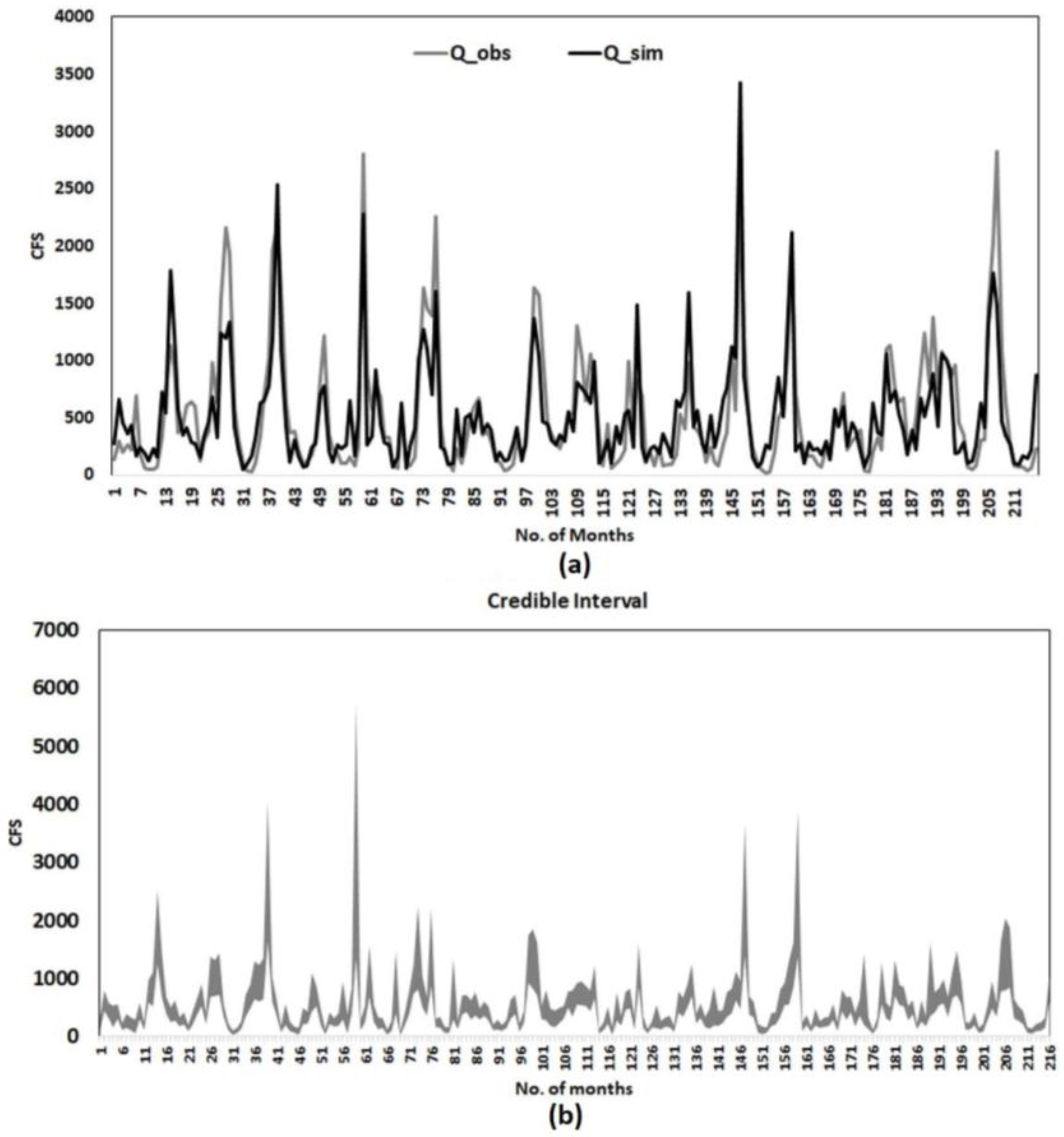
Performance statistics for 12 months, RE, CE and correlation between the model simulated and the observed streamflow, are presented in Table 2. RE and CE values within 0 to 1 indicates that the model performs better than the climatology. BMLS exhibits CE and RE values lower than 1 for all months. However, climatology performs better in May (for RE and CE) and June (for RE alone) as compared to rest of the months. Improved performance of climatology during May and June could be linked with the high variability across consecutive low and high flow months. For the remaining months, the BMLS model is superior to the climatology with CE and RE values around 0.6. During high flow months of March and April, CE values are 0.68 and 0.63 respectively. RE values remain similar to CE values during March and April. The BMLS model exhibits a strong correlation between the observed and model simulated streamflow, except for May, June, and October. Correlation values are 0.51, 0.58 and 0.50 respectively for May, June, and October. Note that, we present the result for the validation period when the performance of the model depends more on the watershed information than climate inputs [35]. Figure 3a shows the time series of model-simulated and observed streamflow. The credible interval of the model simulated streamflow is plotted in Figure 3b. Mean of the probabilistic prediction is used for plotting Figure 3a. The time series of the model simulated streamflow matches with the time series of observed records. However, the BMLS model exhibits weakness in modeling the low extremes. The credible interval is realistic to model the extreme observed streamflow within the range of model uncertainty.
4.2. Comparison Between Hindcast and Historical Runs
In this sub-section, we analyze the role of historical and hindcast simulations as covariates of the BMLS model. As in Section 4.1, the BMLS model is first trained with observed streamflow and observed, gridded pr and tas data for the period 1951–1980. Secondly, the model is tested with gridded pr and tas values from the CMIP5 historical and hindcast run for the period 1981–1999. Hindcast and historical run outputs are obtained from three GCMs, CMRM, IPSL, and MPI. GCM datasets are bias-corrected by applying the ACCA approach to preserve the cross-correlation between pr and tas in the bias-corrected products. CE is used to compare the performance of hindcast and historical outputs in simulating streamflow. The equation (Equation (10)) of CE is now modified to compare root-mean-square error (RMSE) values resulting from hindcast and historical runs. The modified definition of CE is as follows
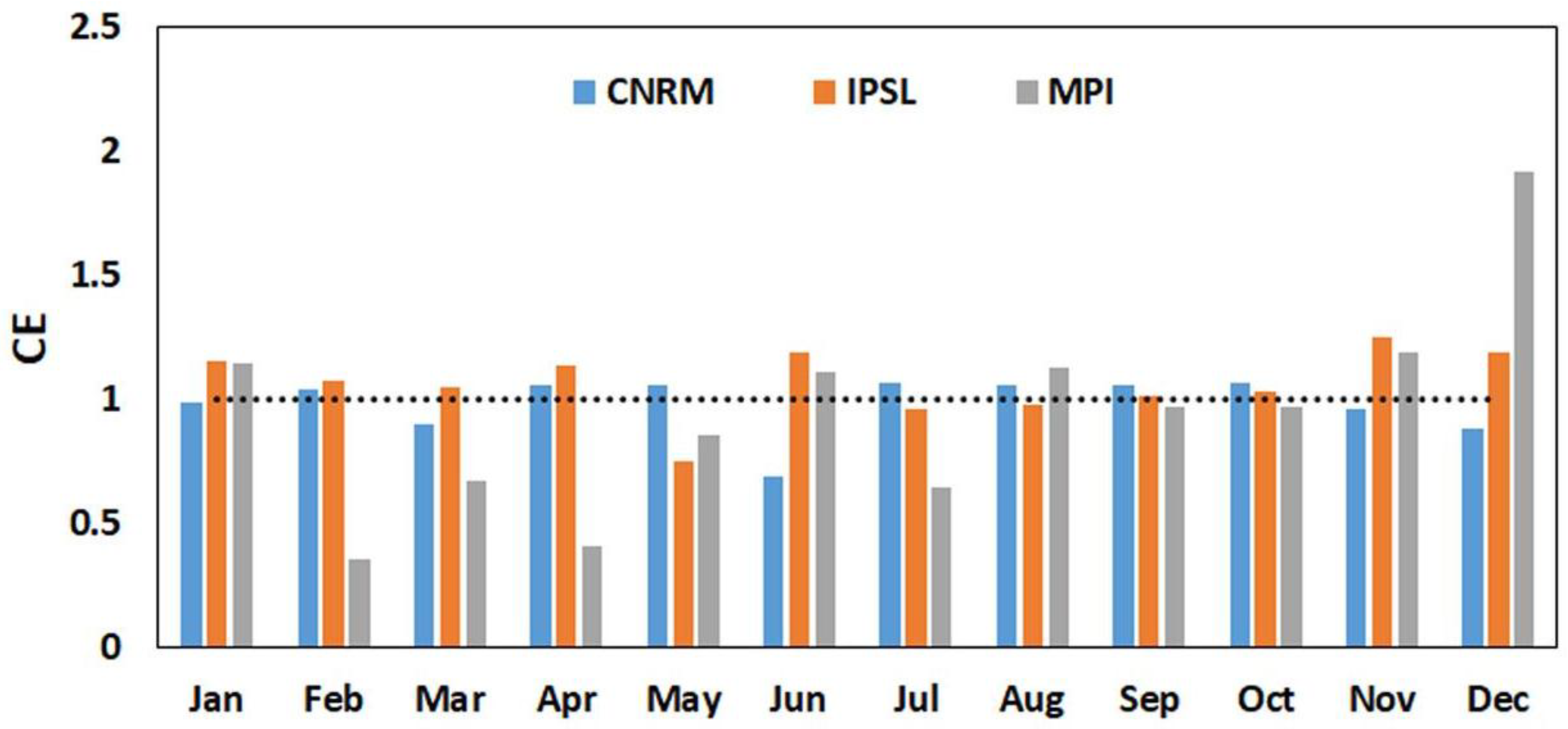
According to Equation (12), a value of CE lesser than 1 indicates that hindcast co-variates result in an improved simulation of streamflow as compared to the historical co-variates. Results are presented in Figure 4.
CNRM and IPSL exhibit CE values higher than 1 for most of the months indicating historical runs have lower values of RMSE compared to the RMSE values from hindcast runs. However, the hindcast runs show improved performance over the historical run for the climate model MPI across seven out of 12 months. During the high flow months, March and April, IPSL historical runs perform better than hindcast runs. In conclusion, results of streamflow simulation with hindcast and historical runs show that the quality of climate prediction is not increased by the SST initialization of climate models. Overall, the results of the analysis are mixed with historical runs performing slightly better than hindcast runs. Reasons for the similar performance of the historical and hindcast runs is linked to the efficient bias-correction of pr and tas using ACCA [22]. The bias-correction yields observed mean, standard deviation and cross-correlation in the bias-corrected hindcast and historical runs.
4.3. Estimation of Future Changes
Finally, we estimate the future changes in streamflow at the HCDN site resulted from the increased greenhouse gas emission. We consider future projections from 12 climate models as inputs to the Bayesian model. BMLS is trained with the observed streamflow, pr, and tas data for the period 1951–1999. The predictor set of the model, as described in Section 3 (Equations (1) and (2)), is modified to project future streamflow. We excluded the lagged-streamflow from the predictor set since observed streamflow values are not available for a large part of the ‘future prediction’ period. To address the modification, we recalibrate the model for the period 1951–1999 using pr and tas as model inputs. Model efficiency (results not presented) is slightly decreased by the exclusion of lagged-streamflow as compared to the results presented in Table 2. However, RE and CE values for the retraining exhibits that BMLS still performs better than the climatology.
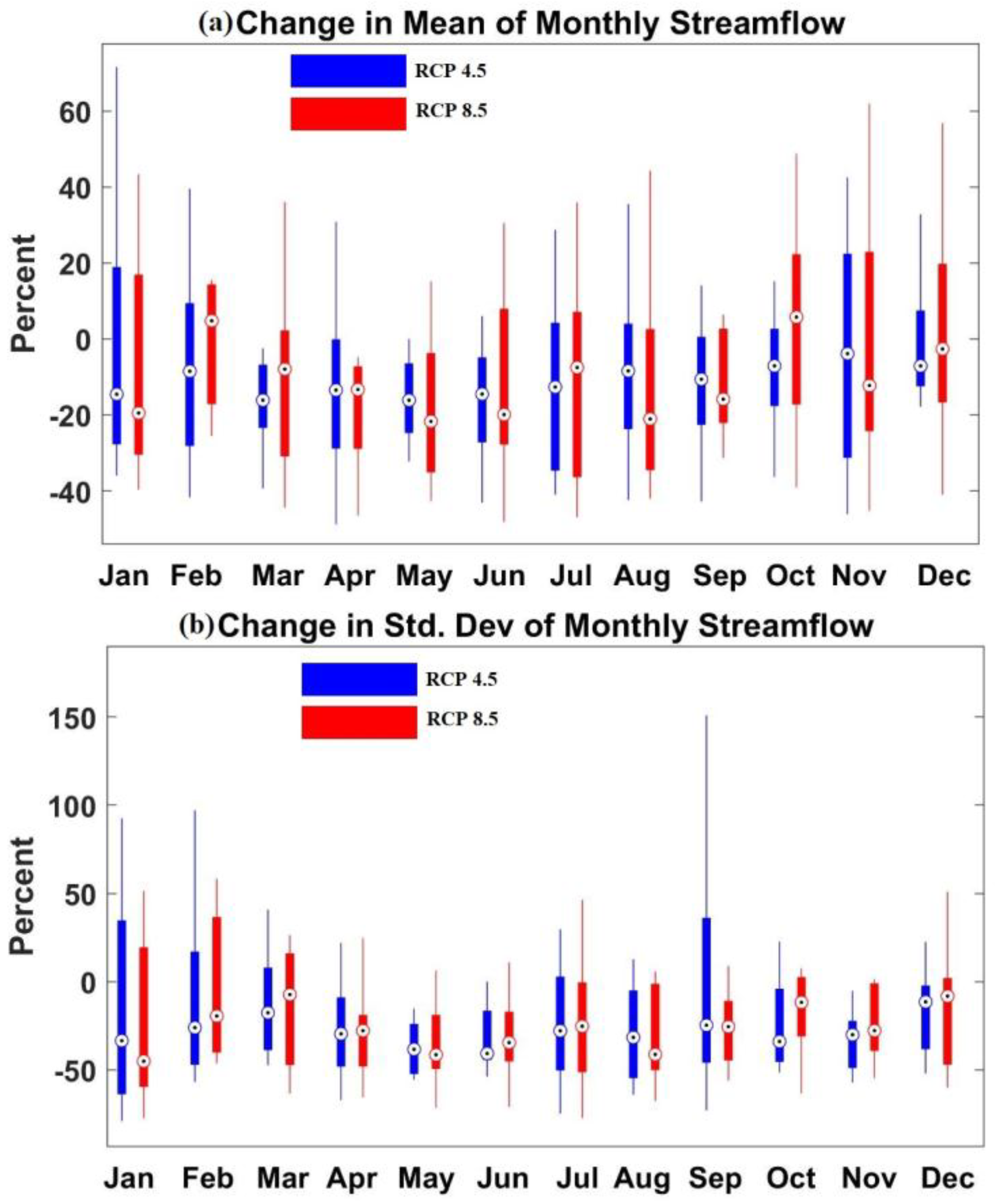
We stored the post burns in MCMC model samples for the training period and used the stored outputs to issue predictions for the future [20]. A set of future streamflow is generated by forcing the BMLS model with pr and tas ensemble projections of a GCM. The study considers two emission scenarios, RCP 4.5 and RCP 8.5. The changes in the streamflow are estimated based on the changes in mean and standard deviation of monthly streamflow (Figure 5). We calculate the following metric, percent change in the streamflow statistics θ where θ is either the mean or the standard deviation.
Percent change is calculated for individual GCMs and presented as boxplots. Blue boxes are for the emission scenario RCP 4.5, while the red boxes represent the emission scenario RCP8.5. Results show that the HCDN site witnesses a decrease in the mean of monthly streamflow over all the months. During January and November, the inter-quartile range of percent change is higher as compared to other months, resulting from the GCM uncertainty. The decrease in the monthly streamflow could reach up to 25%. Projected changes in the mean of monthly streamflow differ by slightly (between 5% and 10%) between emission scenarios RCP4.5 and RCP8.5.
Two emission scenarios project similar values of percent change in the standard deviation (Figure 5b). RCP 4.5 and 8.5 project a reduction in the variability of the monthly streamflow for most of the months. Model uncertainty in projecting streamflow is higher during winter months as compared to other seasons. However, for both scenarios, some of the GCMs indicate a decrease in the variability, based on the range of the percent change. The decrease in the variability in future is within 40% as compared to the last half of the 20th century. In conclusion, the mean and variability in streamflow are expected to be lower in future under different greenhouse gas emission scenarios.
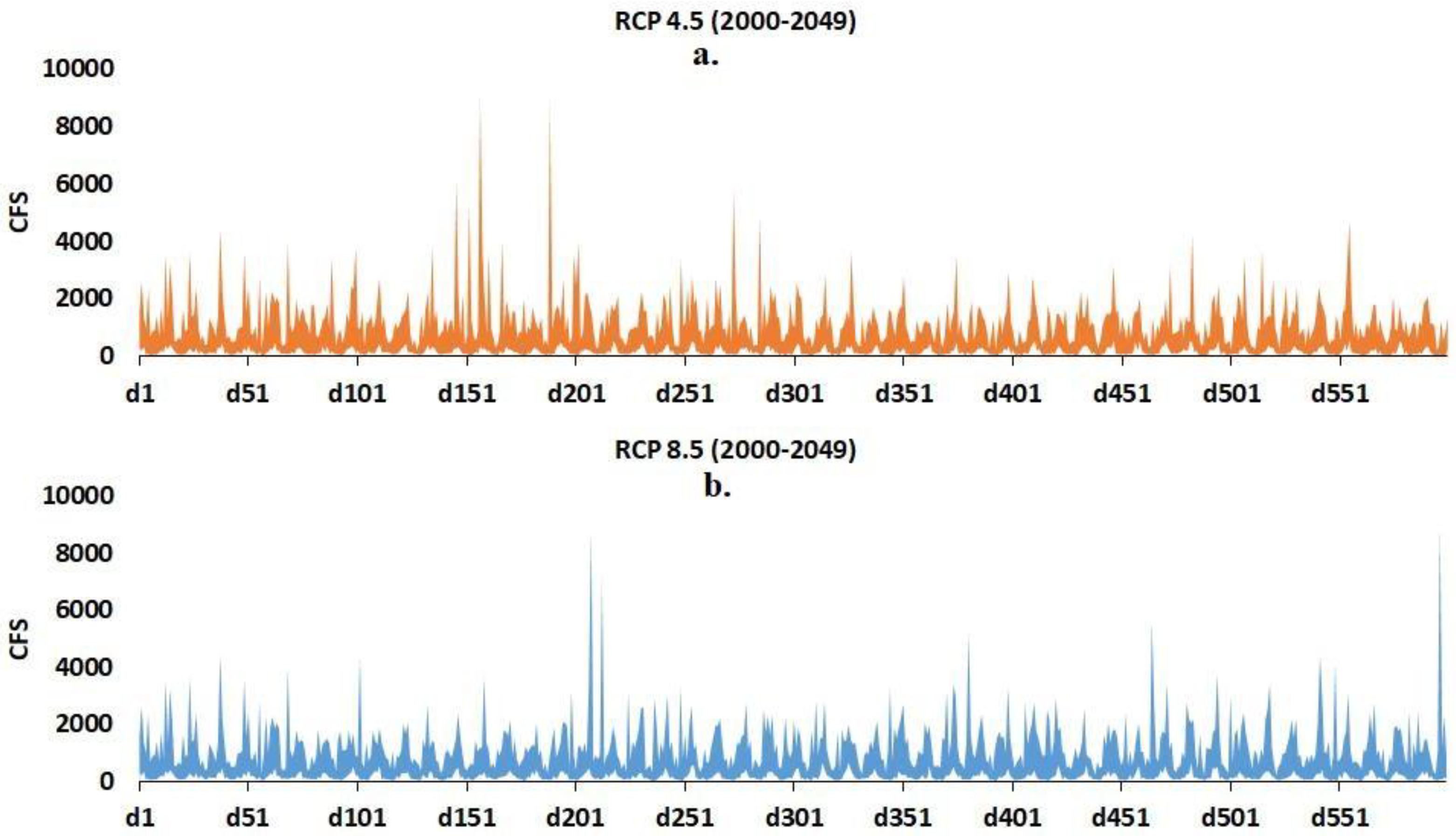
We plot a time-series of the projected streamflow based on the mean of a streamflow ensemble (Figure 6). A streamflow ensemble is generated by forcing the BMLS model with ensemble projection from a climate model. The set of ensembles from 12 climate models leads to a set of 12 streamflow ensembles. Hence, twelve corresponding mean streamflow values are available during a particular month to estimate the GCM uncertainty in projecting the future streamflow. We calculate the maximum and minimum values from the set of mean streamflow to construct a range of expected monthly streamflows (Figure 6). Results show that the GCM uncertainty is significantly large in projecting the future streamflow for both RCP scenarios. For observed streamflow values for 1951–1999, readers are referred to Figure 3a. Note that, GCM 20th century run and future projections under different RCPs exhibit a temporal mismatch with the observed records and with each other. The model uncertainty in projected streamflow can be reduced by adopting a performance-based multi-model combination approach or simply by applying equal weight to ensemble members [36].
5. Discussion
In this study, we modified and applied a novel statistical approach, BMLS, for monthly streamflow simulation. The BMLS model is applied for long-term streamflow simulation on an HCDN basin with lagged-streamflow, precipitation and temperature variables (for the future period, only precipitation and temperature) being the predictors. Firstly, we validated the BMLS model for the period 1951–1980 using observed precipitation and temperature and lagged observed streamflow inputs. Secondly, monthly streamflow is simulated by forcing GCM outputs from historical and hindcast experiments for the model validation period. Finally, future changes in streamflow are estimated based on future projections from twelve GCMs. The BMLS model is recalibrated with climate data (excluding lagged streamflow) from historical period (1951–1999) to project future changes streamflow for the period 2000–2049. Precipitation and temperature projections under two RCP scenarios (RCP 4.5 and RCP 8.5) from 12 GCMs are considered as predictors. Projected changes in the climate predictors have resulted from human-induced climate change. Hence, the changes in streamflow are also linked with the anthropogenic changes which are represented from RCP scenarios.
Validation results show that simulated streamflow exhibits significant information that is not presented in the climatology of the calibration or validation periods. The BMLS model exhibits RE and CE values lesser than one across all months during the validation period. Simulated and observed streamflow share a strong correlation during the validation period, except May, June, and October. Three-fold cross-validation, implemented to avoid the over-fitting of the model, exhibits a consistent performance of the BMLS model across the three validation sets. Results of streamflow simulations on the HCDN station, forced with GCM outputs, show that hindcast runs generally perform no better than the historical runs. Only one GCM hindcast, MPI, perform better than the GCM historical run on seven out of 12 months. The mean and the variability of streamflow on the HCDN basin is expected to decrease in future (2000–2049) under RCP 4.5 and 8.5. Percent change in future moments of monthly streamflow is estimated to be within 25% (40%) for the mean (standard deviation). The mean and variability of monthly streamflow on the gauging site are expected to decrease during 2000–2049. Changes in the streamflow could be associated with a future decrease in precipitation intensity, increase in the number of dry days across the south-east, and an increase in the average temperature. Swain and Hayhoe [37] reported statistically significant increases in the mean spring standard precipitation index (SPI) over the northern part of the North American continent. Earlier studies have estimated a similar magnitude of change in river flow for the near, mid and long-term future. Campbell et al. [38] predicted a change of −11% to +1% in the annual streamflow over a small watershed in the north-eastern United States. The magnitude and slope of the future change in streamflow depend substantially on the hydro-climate. For example, Chase et al. [39] reported that two out of seven watersheds of eastern and central Montana would experience a decrease in the mean annual streamflow in the future, while the rest of the watersheds would experience an increase (decrease) in mean annual streamflow for the period 2021–2038 (2071–2088). Apart from the mean streamflow, the frequency of minor flooding over the near-term and mid-term future is also expected to increase under two RCPs along the coastal United States [40].
Statistical models, in general, assume stationarity in projecting future changes, hence are not considered to be significantly reliable for climate change impact studies. Additionally, climate model uncertainty and scenario uncertainty result in a significant prediction uncertainty in the future streamflow. Despite the shortcomings of statistical techniques, our study confirms the applicability of the BMLS model for long-term streamflow simulation. Model calibration and validation results indicate that the model could be useful when the watershed information is limited, and a large number of climate predictors are present. Consistent performance of the model leads us to perform additional experiments with CMIP5′s historical and hindcast runs. We suggest that no further benefit can be achieved in streamflow simulation by replacing historical runs with decadal predictions. Nevertheless, hindcast projections are useful for streamflow simulations of 30 years or less. For a simulation of more than 30 years, the study suggests using long-term climate projections to estimate the future changes. A decrease in the monthly streamflow would result in additional stress on water resources planning. A future study should examine the impact of the reduction in the mean of monthly streamflow on downstream reservoirs, and the soft and hard-path strategies to replenish the deficit.
The BMLS model allows predictors with a spatial resolution different from that of the predictand. Unlike process-based models like SWAT or PIHM, the BMLS model does not necessarily require pre-processing of climate model outputs. Such pre-processing may include predictor selections, bias-correction and spatial downscaling, etc. Earlier studies have reported that the pre-processing of climate predictors can potentially include significant uncertainty in the streamflow simulation [26,41,42]. However, the current study has applied a multivariate bias-correction technique, ACCA, to remove model bias in climate predictors while preserving the interdependence between precipitation and temperature. A future study to evaluate the difference between the hindcast and historical runs should include multiple stream-gauge sites to provide a comprehensive understanding of the problem. The current study does not estimate the statistical significance of the CE values estimated using hindcast and historical runs (Section 4.2). A non-parametric bootstrap approach can be applied to test the statistical significance of the CE values. The null hypothesis would state that CE value is equal to one, i.e., RMSE exhibited by hindcast, and historical runs are the same. Readers are encouraged to read Goddard et al. [23] for details regarding the non-parametric bootstrap approach in the context of a decadal experiment’s verification. The similar performance of historical and hindcast runs as climate predictors are attributed to the efficiency of the ACCA technique because predictor uncertainty is considered as one of the dominant sources of the uncertainty in simulated streamflow [26]. In conclusion, the quality of GCM outputs eventually does not vary between SST initialized and non-initialized climate model runs.
Future improvement of the current model can be achieved by considering informative prior selection, incorporating predictor selection algorithms and adopting a sensitivity analysis to achieve a thorough understanding of the model parameters. Although the current study considers a single station, selection of multiple HCDN stations across various climate regions of the United States would provide a comprehensive understanding of the reversibility of the BMLS model on multiple basins. Including climate indices and teleconnection, such as SST, ENSO, and PDO, is expected to ensure an improved simulation of streamflow. Predictor uncertainty can be reduced by considering observed climate variables with finer resolution. An increase in the number of GCMs for future assessment is expected to reduce the model uncertainty and improve accuracy [43,44,45,46,47]. Finally, the study confirms the applicability of a novel Bayesian approach for streamflow simulation and concludes that the approach can be useful in assessing the impacts of climate change on water resources.
Author Contributions
Conceptualization, R.D.B., S.B.S., and S.S.; Methodology, S.S., R.D.B., and S.B.S; Data compilation, S.B.S., and R.D.B; Computation, R.D.B., and S.B.S.; Writing-Original Draft Preparation, R.D.B., S.S., and S.B.S..; Writing-Review & Editing, R.D.B., S.S., and S.B.S.; Funding Acquisition, S.B.S.
Funding
This research was supported by a grant (NRF-2017R1A6A3A11031800) through the Young Researchers program funded by the National Research Foundation of Korea.
Acknowledgments
We acknowledge the World Climate Research Programme’s Working Group on Coupled Modelling, which is responsible for CMIP, and we thank the climate modeling groups (listed in Table 1) for producing and making available their model output. For CMIP the U.S. Department of Energy’s Program for Climate Model Diagnosis and Intercomparison provides coordinating support and led the development of software infrastructure in partnership with the Global Organization for Earth System Science Portals. “Downscaled CMIP3 and CMIP5 Climate and Hydrology Projections” archive at http://gdo-dcp.ucllnl.org/downscaled_cmip_projections/ (accessed on 23 April 2017). We also thank the two anonymous reviewers and the Academic Editor for their comments and detailed reviews, which led to substantial improvements in the quality of the manuscript.
Conflicts of Interest
The authors declare no conflict of interest.
References
- Kim, B.S.; Kim, H.S.; Seoh, B.H. Streamflow Simulation and Skewness Preservation Based on the Bootstrapped Stochastic Models. Stoch. Environ. Res. Risk Assess. 2004, 18, 386–400. [Google Scholar] [CrossRef]
- Schubert, S.; Koster, R.; Hoerling, M.; Seager, R.; Lettenmaier, D.; Kumar, A.; Gutzler, D. Predicting drought on seasonal-to-decadal time scales. Bull. Am. Meteorol. Soc. 2007, 88, 1625–1630. [Google Scholar] [CrossRef]
- Wang, S.; Zhang, Z.R.; McVicar, T.; Guo, J.; Tang, Y.; Yao, A. Isolating the Impacts of Climate Change and Land Use Change on Decadal Streamflow Variation: Assessing Three Complementary Approaches. J. Hydrol. 2013, 507, 63–74. [Google Scholar] [CrossRef]
- Devia, G.K.; Ganasri, B.P.; Dwarakish, G.S. ScienceDirect ScienceDirect A Review on Hydrological Models. Aquat. Procedia 2015, 4, 1001–1007. [Google Scholar] [CrossRef]
- Iorgulescu, I.; Beven, K.J. Nonparametric Direct Mapping of Rainfall-Runoff Relationships: An Alternative Approach to Data Analysis and Modeling? Water Resour. Res. 2004, 40. [Google Scholar] [CrossRef]
- See, L.; Solomatine, D.; Abrahart, R.; Toth, E. Hydroinformatics: Computational Intelligence and Technological Developments in Water Science applications—Editorial. Hydrol. Sci. J. 2007, 52, 391–396. [Google Scholar] [CrossRef]
- Sharma, A.; Tarboton, D.G.; Lall, U. Streamflow Simulation: A Nonparametric Approach. Water Resour. Res. 1997, 33, 291–308. [Google Scholar] [CrossRef]
- Hirsch, R.M. Stochastic Hydrologic Model for Drought. J. Water Resour. Plan. Manag. Div. 1981, 107, 303–313. [Google Scholar]
- Tasker, G.D. A comparison of methods for estimating low flow characteristics of streams. J. Am. Water Resour. Assoc. 1987, 23, 1077–1083. [Google Scholar] [CrossRef]
- Woo, M.K. Confidence Intervals of Optimal Risk-Based Hydraulic Design Parameters. Can. Water Resour. 1989, 14, 10–16. [Google Scholar] [CrossRef]
- Cover, K.A.; Unny, T.E. Application of computer intensive statistics to parameter uncertainty in streamflow synthesis. J. Am. Water Resour. Assoc. 1986, 22, 495–507. [Google Scholar] [CrossRef]
- Kong, X.M.; Huang, G.H.; Fan, Y.R.; Li, Y.P. Maximum Entropy-Gumbel-Hougaard Copula Method for Simulation of Monthly Streamflow in Xiangxi River, China. Stoch. Environ. Res. Risk Assess. 2015, 29, 833–846. [Google Scholar] [CrossRef]
- Li, H.-S. Maximum Entropy Method for Probabilistic Bearing Strength Prediction of Pin Joints in Composite Laminates. Compos. Struct. 2013, 106, 626–634. [Google Scholar] [CrossRef]
- Shortridge, J.E.; Guikema, S.D.; Zaitchik, B.F. Machine Learning Methods for Empirical Streamflow Simulation: A Comparison of Model Accuracy, Interpretability, and Uncertainty in Seasonal Watersheds. Hydrol. Earth Syst. Sci. 2016, 20, 2611–2628. [Google Scholar] [CrossRef]
- Asefa, T.; Kemblowski, M.; McKee, M.; Khalil, A. Multi-Time Scale Stream Flow Predictions: The Support Vector Machines Approach. J. Hydrol. 2006, 318, 7–16. [Google Scholar] [CrossRef]
- Lin, J.-Y.; Cheng, C.-T.; Chau, K.-W. Using Support Vector Machines for Long-Term Discharge Prediction. Hydrol. Sci. J. 2006, 51, 599–612. [Google Scholar] [CrossRef]
- Galelli, S.; Castelletti, A. Tree-Based Iterative Input Variable Selection for Hydrological Modeling. Water Resour. Res. 2013, 49, 4295–4310. [Google Scholar] [CrossRef]
- Solomatine, D.P.; Ostfeld, A. Data-Driven Modelling: Some Past Experiences and New Approaches. J. Hydroinform. 2008, 10, 3–22. [Google Scholar] [CrossRef]
- Sudheer, K.P.; Jain, A. Explaining the Internal Behaviour of Artificial Neural Network River Flow Models. Hydrol. Process. 2004, 18, 833–844. [Google Scholar] [CrossRef]
- Holmes, C.C.; Mallick, B.K. Bayesian Regression with Multivariate Linear Splines. J. R. Stat. Soc. Ser. B 2001, 63, 3–17. [Google Scholar] [CrossRef]
- Taylor, K.E.; Stouffer, R.J.; Meehl, G.A.; Taylor, K.E.; Stouffer, R.J.; Meehl, G.A. An Overview of CMIP5 and the Experiment Design. Bull. Am. Meteorol. Soc. 2012, 93, 485–498. [Google Scholar] [CrossRef] [Green Version]
- Das Bhowmik, R.; Sankarasubramanian, A.; Sinha, T.; Patskoski, J.; Mahinthakumar, G.; Kunkel, K.E. Multivariate Downscaling Approach Preserving Cross Correlations across Climate Variables for Projecting Hydrologic Fluxes. J. Hydrometeorol. 2017, 18, 2187–2205. [Google Scholar] [CrossRef]
- Goddard, L.; Kumar, A.; Solomon, A.; Smith, D.; Boer, G.; Gonzalez, P.; Kharin, V.; Merryfield, W.; Deser, C.; Mason, S.J.; et al. A Verification Framework for Interannual-to-Decadal Predictions Experiments. Clim. Dyn. 2013, 40, 245–272. [Google Scholar] [CrossRef] [Green Version]
- Slack, J.; Landwehr, J. Hydro-Climatic Data Network (HCDN); A US Geological Survey Streamflow Data Set for the United States for the Study of Climate Variations; US Geological Survey: Reston, VA, USA, 1992; pp. 1874–1988.
- Sankarasubramanian, A.; Vogel, R.M. Annual Hydroclimatology of the United States. Water Resour. Res. 2002, 38, 19-1–19-12. [Google Scholar] [CrossRef]
- Seo, S.B.; Sinha, T.; Mahinthakumar, G.; Sankarasubramanian, A.; Kumar, M. Identification of Dominant Source of Errors in Developing Streamflow and Groundwater Projections under near-Term Climate Change. J. Geophys. Res. Atmos. 2016, 121, 7652–7672. [Google Scholar] [CrossRef]
- Li, W.; Sankarasubramanian, A.; Ranjithan, R.S.; Sinha, T. Role of Multimodel Combination and Data Assimilation in Improving Streamflow Prediction over Multiple Time Scales. Stoch. Environ. Res. Risk Assess. 2016, 30, 2255–2269. [Google Scholar] [CrossRef]
- Maurer, E.P.; Wood, A.W.; Adam, J.C.; Lettenmaier, D.P.; Nijssen, B.; Maurer, E.P.; Wood, A.W.; Adam, J.C.; Lettenmaier, D.P.; Nijssen, B. A Long-Term Hydrologically Based Dataset of Land Surface Fluxes and States for the Conterminous United States. J. Clim. 2002, 15, 3237–3251. [Google Scholar] [CrossRef]
- Das Bhowmik, R. Reducing Downscaling & Model Uncertainties in CMIP5 Decadal Hindcasts/Projections. Doctoral Dissertation. Available online: http://www.lib.ncsu.edu/resolver/1840.20/33329 (accessed on 10 November 2017).
- Giorgi, F.; Mearns, L.O. Probability of Regional Climate Change Based on the Reliability Ensemble Averaging (REA) Method. Geophys. Res. Lett. 2003, 30. [Google Scholar] [CrossRef]
- Tebaldi, C.; Knutti, R. The Use of the Multi-Model Ensemble in Probabilistic Climate Projections. Philos. Trans. A Math. Phys. Eng. Sci. 2007, 365, 2053–2075. [Google Scholar] [CrossRef] [PubMed]
- Jun, M.; Knutti, R.; Nychka, D.W. Spatial Analysis to Quantify Numerical Model Bias and Dependence: How Many Climate Models Are There? J. Am. Stat. Assoc. 2008, 103, 934–947. [Google Scholar] [CrossRef]
- Räisänen, J.; Ruokolainen, L.; Ylhäisi, J. Weighting of Model Results for Improving Best Estimates of Climate Change. Clim. Dyn. 2010, 35, 407–422. [Google Scholar] [CrossRef]
- Chen, X.; Hao, Z.; Devineni, N.; Lall, U. Climate Information Based Streamflow and Rainfall Forecasts for Huai River Basin Using Hierarchical Bayesian Modeling. Hydrol. Earth Syst. Sci. 2014, 18, 1539–1548. [Google Scholar] [CrossRef]
- Chen, J.; Li, C.; Brissette, F.P.; Chen, H.; Wang, M.; Essou, G.R. Impacts of correcting the inter-variable correlation of climate model outputs on hydrological modeling. J. Hydrol. 2018, 560, 326–341. [Google Scholar] [CrossRef]
- Bhowmik, R.D.; Sharma, A.; Sankarasubramanian, A. Reducing Model Structural Uncertainty in Climate Model Projections—A Rank-Based Model Combination Approach. J. Clim. 2017, 30, 10139–10154. [Google Scholar] [CrossRef]
- Swain, S.; Hayhoe, K. CMIP5 projected changes in spring and summer drought and wet conditions over North America. Clim. Dyn. 2015, 44, 2737–2750. [Google Scholar] [CrossRef]
- Campbell, J.L.; Driscoll, C.T.; Pourmokhtarian, A.; Hayhoe, K. Streamflow responses to past and projected future changes in climate at the Hubbard Brook Experimental Forest, New Hampshire, United States. Water Resour. Res. 2011, 47. [Google Scholar] [CrossRef] [Green Version]
- Chase, K.J.; Haj, A.E.; Regan, R.S.; Viger, R.J. Potential effects of climate change on streamflow for seven watersheds in eastern and central Montana. J. Hydrol. 2016, 7, 69–81. [Google Scholar] [CrossRef]
- Moftakhari, H.R.; AghaKouchak, A.; Sanders, B.F.; Feldman, D.L.; Sweet, W.; Matthew, R.A.; Luke, A. Increased nuisance flooding along the coasts of the United States due to sea level rise: Past and future. Geophys. Res. Lett. 2015, 42, 9846–9852. [Google Scholar] [CrossRef] [Green Version]
- Singh, H.; Sankarasubramanian, A. Systematic Uncertainty Reduction Strategies for Developing Streamflow Forecasts Utilizing Multiple Climate Models and Hydrologic Models. Water Resour. Res. 2014, 50, 1288–1307. [Google Scholar] [CrossRef]
- Mazrooei, A.; Sinha, T.; Sankarasubramanian, A.; Kumar, S.; Peters-Lidard, C.D. Decomposition of Sources of Errors in Seasonal Streamflow Forecasting over the U.S. Sunbelt. J. Geophys. Res. Atmos. 2015, 120, 11809–11825. [Google Scholar] [CrossRef]
- Krishnamurti, T.N.; Kishtawal, C.M.; LaRow, T.E.; Bachiochi, D.R.; Zhang, Z.; Williford, C.E.; Gadgil, S.; Surendran, S. Improved Weather and Seasonal Climate Forecasts from Multimodel Superensemble. Science 1999, 285, 1548–1550. [Google Scholar] [CrossRef] [PubMed]
- Doblas-Reyes, F.J.; Déqué, M.; Piedelievre, J.-P. Multi-Model Spread and Probabilistic Seasonal Forecasts in PROVOST. Q. J. R. Meteorol. Soc. 2010, 126, 2069–2087. [Google Scholar] [CrossRef]
- Palmer, T.N.; Branković, Č.; Richardson, D.S. A Probability and Decision-Model Analysis of PROVOST Seasonal Multi-Model Ensemble Integrations. Q. J. R. Meteorol. Soc. 2010, 126, 2013–2033. [Google Scholar] [CrossRef]
- Rajagopalan, B.; Lall, U.; Zebiak, S.E.; Rajagopalan, B.; Lall, U.; Zebiak, S.E. Categorical Climate Forecasts through Regularization and Optimal Combination of Multiple GCM Ensembles. Mon. Weather Rev. 2002, 130, 1792–1811. [Google Scholar] [CrossRef]
- Barnston, A.G.; Mason, S.J.; Goddard, L.; Dewitt, D.G.; Zebiak, S.E. Multimodel Ensembling in Seasonal Climate Forecasting at IRI. Bull. Am. Meteorol. Soc. 2003, 84, 1783–1796. [Google Scholar] [CrossRef] [Green Version]
Figure 1.
(a) Map of the Nottoway River basin, including the Hydroclimate Data Network (HCDN) site (gauge station) and grid cells of climate variables. (b) Climatology of streamflow on the site estimated for the period 1951–1980.
Figure 1.
(a) Map of the Nottoway River basin, including the Hydroclimate Data Network (HCDN) site (gauge station) and grid cells of climate variables. (b) Climatology of streamflow on the site estimated for the period 1951–1980.

Figure 2.
Schematic diagram of the experimental design. The ‘validation’ block is repeated three times by altering different training and testing dataset to achieve three-fold cross-validation.
Figure 2.
Schematic diagram of the experimental design. The ‘validation’ block is repeated three times by altering different training and testing dataset to achieve three-fold cross-validation.

Figure 3.
(a) Time series of simulated and observed monthly streamflow for the validation period 1981–1999; (b) credible interval of the simulated streamflow.
Figure 3.
(a) Time series of simulated and observed monthly streamflow for the validation period 1981–1999; (b) credible interval of the simulated streamflow.

Figure 4.
Co-efficient of efficiency (CE) exhibited by three general circulation models (GCMs) for the period 1981–1999. CE is calculated using root-mean-square error (RMSE) values of simulated streamflow forced with hindcast and historical runs. CE value lesser than 1 indicates that hindcast co-variates result in an improved simulation of streamflow as compared to the historical co-variates. CE is estimated for each member within a GCM ensemble (numbers of ensemble members is provided in Table 1), and the average value of CE is calculated.

Figure 5.
Boxplots show the percent change in the moments of monthly streamflow for the period 2000–2049 w.r.t the moments of monthly streamflow for 1951–1999. (a) Changes in the mean; (b) changes in the standard deviation. Twelve GCMs are used for the analysis. Percent change is estimated for each member within a GCM ensemble (numbers of ensemble members is provided in Table 1).

Figure 6.
Time-series of Bayesian regression with multivariate linear spline (BMLS) projected future streamflow (2000–2049) under (a) RCP 4.5 and (b) RCP 8.5. Twelve GCMs are used in the analysis. Maximum and minimum values from a set of twelve mean streamflow values are estimated to construct the projection uncertainty band.


Table 1.
Description of general circulation model (GCM) dataset.
| Model Name | Experiment | Time Length | Ensemble Members |
|---|---|---|---|
| CNRM-CM5 | Historical | 1950–1999 | 5 |
| Hindcast (Decadal 80) | 1981–1999 | 9 | |
| Future Projections (RCP 4.5 & 8.5) | 2000–2049 | 2 | |
| MRI-ESR-LR | Historical | 1950–1999 | 1 |
| Hindcast (Decadal 80) | 1981–1999 | 3 | |
| Future Projections (RCP 4.5 & 8.5) | 2000–2049 | 6 | |
| IPSL-CM-LR | Historical | 1950–1999 | 4 |
| Hindcast (Decadal 80) | 1981–1999 | 6 | |
| Future Projections (RCP 4.5 & 8.5) | 2000–2049 | 2 | |
| ACCESS 1-0 | Future Projections (RCP 4.5 & 8.5) | 2000–2049 | 2 |
| BCC-CSM 1-1 | Future Projections (RCP 4.5 & 8.5) | 2000–2049 | 2 |
| CANESM 2 | Future Projections (RCP 4.5 & 8.5) | 2000-2049 | 10 |
| CMCC-CM | Future Projections (RCP 4.5 & 8.5) | 2000–2049 | 2 |
| EC-EARTH | Future Projections (RCP 4.5 & 8.5) | 2000–2049 | 6 |
| HADGEM2-CC | Future Projections (RCP 4.5 & 8.5) | 2000–2049 | 2 |
| MIROC-5 | Future Projections (RCP 4.5 & 8.5) | 2000–2049 | 2 |
| MRI-CGEM3 | Future Projections (RCP 4.5 & 8.5) | 2000–2049 | 2 |
| NORESM1-MC | Future Projections (RCP 4.5 & 8.5) | 2000–2049 | 2 |
Table 2.
Performance statistics of Bayesian regression with multivariate linear spline (BMLS) during validation.
Table 2.
Performance statistics of Bayesian regression with multivariate linear spline (BMLS) during validation.
| January | February | March | April | May | June | July | August | September | October | November | December | |
|---|---|---|---|---|---|---|---|---|---|---|---|---|
| CE | 0.77 | 0.69 | 0.68 | 0.63 | 0.78 | 0.51 | 0.54 | 0.69 | 0.47 | 0.77 | 0.39 | 0.81 |
| RE | 0.77 | 0.70 | 0.69 | 0.63 | 0.97 | 0.72 | 0.67 | 0.93 | 0.49 | 0.95 | 0.39 | 0.85 |
| Corr | 0.73 | 0.72 | 0.77 | 0.91 | 0.51 | 0.58 | 0.57 | 0.52 | 0.98 | 0.50 | 0.96 | 0.63 |
© 2018 by the authors. Licensee MDPI, Basel, Switzerland. This article is an open access article distributed under the terms and conditions of the Creative Commons Attribution (CC BY) license (http://creativecommons.org/licenses/by/4.0/).
Share and Cite
MDPI and ACS Style
Das Bhowmik, R.; Seo, S.B.; Sahoo, S. Streamflow Simulation Using Bayesian Regression with Multivariate Linear Spline to Estimate Future Changes. Water 2018, 10, 875. https://doi.org/10.3390/w10070875
AMA Style
Das Bhowmik R, Seo SB, Sahoo S. Streamflow Simulation Using Bayesian Regression with Multivariate Linear Spline to Estimate Future Changes. Water. 2018; 10(7):875. https://doi.org/10.3390/w10070875
Chicago/Turabian StyleDas Bhowmik, Rajarshi, Seung Beom Seo, and Saswata Sahoo. 2018. "Streamflow Simulation Using Bayesian Regression with Multivariate Linear Spline to Estimate Future Changes" Water 10, no. 7: 875. https://doi.org/10.3390/w10070875
Note that from the first issue of 2016, this journal uses article numbers instead of page numbers. See further details here.