Inlet Water Quality Forecasting of Wastewater Treatment Based on Kernel Principal Component Analysis and an Extreme Learning Machine

1
College of Environment and Resources, Chongqing Technology and Business University, Chongqing 400067, China
2
National Research Base of Intelligent Manufacturing Service, Chongqing Technology and Business University, Chongqing 400067, China
3
Chongqing Water Asset Management Co., Ltd., Chongqing 400015, China
*
Author to whom correspondence should be addressed.
Water 2018, 10(7), 873; https://doi.org/10.3390/w10070873
Submission received: 22 May 2018
/
Revised: 20 June 2018
/
Accepted: 26 June 2018
/
Published: 30 June 2018
(This article belongs to the Section Water Quality and Contamination)
Abstract
:The stable operation of sewage treatment is of great significance to controlling regional water environment pollution. It is also important to forecast the inlet water quality accurately, which may ensure the purification efficiency of sewage treatment at a low cost. In this paper, a combined kernel principal component analysis (KPCA) and extreme learning machine (ELM) model is established to forecast the inlet water quality of sewage treatment. Specifically, KPCA is employed for feature extraction and dimensionality reduction of the inlet wastewater quality and ELM is utilized for the future inlet water quality forecasting. The experimental results indicated that the KPCA-ELM model has a higher accuracy than the other comparison PCA-ELM model, ELM model, and back propagation neural network (BPNN) model for forecasting COD and BOD concentration of the inlet wastewater, with mean absolute error (MAE) values of 2.322 mg/L and 1.125 mg/L, mean absolute percentage error (MAPE) values of 1.223% and 1.321%, and root mean square error (RMSE) values of 3.108 and 1.340, respectively. It is recommended from this research that the method may provide a reliable and effective reference for forecasting the water quality of sewage treatment.
1. Introduction
The accumulation of high levels of pollutants in water may cause adverse effects on humans and wildlife [1,2]. It is necessary to purify polluted water by sewage treatment in a timely manner to meet emission standards. However, the production conditions of the sewage treatment process are accompanied by random disturbance. It is difficult to deal with water quality in a short time so that it returns to normal, which will greatly affect the next phase of water quality once the problem occurs and it may result in serious energy waste. The past observation data for forecasting inlet water quality helps to adjust the performance parameters and keep the wastewater treatment plant (WWTP) operating economically and stably. Therefore, inlet water quality forecasting is vital for wastewater treatment [3], which gives messages in advance for guiding the operations with a high efficiency.
Recently, various models for dealing with this issue have been proposed, e.g., artificial neural network [4,5], auto-regressive integrated moving average [6], data mining [3], Multiple regression method [7], adaptive recursive least squares [8], support vector machine [9], partial least squares [10], and measured hydraulic dynamics [11]. Among these models, machine learning has attracted much attention because of its superiorities [12], e.g., high generalization performance, low computational complexity, fast learning speed, strong generalization ability, and universal approximation property [13]. Many machine learning experts have turned to high-level abstractions, which dramatically simplify the design and implementation of a restricted class of parallel algorithms [14]. Machine learning is programming computers to optimize a performance criterion using example data or past experience [15], and an extreme learning machine (ELM) is a successful representation [16]. A new fast learning neural algorithm that refers to the ELM with additive hidden nodes and radial basis function kernels has been developed for single-hidden layer feed forward networks (SLFNs) [17]. It has shown an excellent predictive performance in various fields because of several salient features: (1) Simple structure: No parameters need to be manually tuned except for the predefined network architecture [18]; (2) Fast learning speed: It can produce a good generalization performance in most cases and learn thousands of times faster than conventional popular learning algorithms for feed forward neural networks [19]; and (3) Wide applicability: Almost all piece wise continuous can be used as activation functions in ELM and fully complex functions can also be used as activation functions in ELM. Therefore, it is an active research topic with multiple extensions and improvements proposed over the last decade [20], e.g., horizontal global solar radiation [21], Landslide hazard [22], electricity price [23], short-term load forecasting [24], and water quality [25]. The ELM is applied to forecast the inlet wastewater quality in this paper, and the experimental results have achieved a good effect.
To enhance the forecasting accuracy, many data preprocess methods are proposed in forecasting models, e.g., principal component analysis (PCA) [26], kernel principal component analysis (KPCA) [27], wavelet transform [28], cluster analysis [29], mode decomposition [30], linear discriminant analysis [31], independent component correlation algorithm [32], and factor analysis [33]. Among these techniques, the PCA and the KPCA are widely used in classification, feature extraction, and de-noising applications [34], which can help reduce the dimensionality of the data and determine the key variables in a multidimensional data set [35,36]. Furthermore, compared with the PCA [37], the KPCA can effectively capture data nonlinear characteristics without requirements for the spatial distribution of the original data. The method has been successfully applied in many fields, e.g., process monitoring and fault diagnosis [38], intrusion detection [39], formation drill ability prediction [40], and displacement prediction in colluvial landslides [41]. However, the KPCA is rarely applied to inlet wastewater quality forecasting, so the KPCA is thus introduced in this paper.
Therefore, the ELM model combining the KPCA is proposed for inlet wastewater forecasting. The frameworks of the approach can be divided into two parts: (1) Principal components extraction: Describes the feature extraction case, in which KPCA is introduced as a tool for eliminating linear correlation among data and for extracting the principal components; and (2) Forecasting model performance: Performs the ELM to learn and forecast the inlet wastewater quality factors. In this paper, chemical oxygen demand (COD) and biochemical oxygen demand (BOD) are taken as examples, which are representative parameters for sewer water quality [42,43,44], and the oxygen consumption from the degradation of organic material is normally measured as BOD and COD. So, the BOD and the COD are selected as forecasting quality factors in this paper. Furthermore, to validate performance, the investigated results are compared with the PCA-ELM, the ELM, and the back propagation neural network (BPNN) in this study.
The remainder of this paper is structured as follows. Section 2 describes the modeling methods of the KPCA, ELM, and proposed KPCA-ELM models. Section 3 illustrates the datasets, the process of sewage treatment, the experimental design, and the performance criteria of the forecasting models. Section 4 presents the search results and discussion. Section 5 provides conclusions.
2. Materials and Methods
2.1. Extracting Principal Components Based on KPCA
The KPCA has successfully extended the PCA to nonlinear cases by mapping the data in the original space into a higher or even infinite dimensional feature space [45]. This mapping technique can increase the amount of information in the data set, particularly if the number of data is small [46]. The KPCA has already proven to be powerful as a preprocessing step for identification algorithms [47,48,49]. In this section, a brief description of KPCA for feature extraction is provided.
A sample composed of n particles is represented as xk (k = 1, 2, 3, …, n). Assuming φ is nonlinear mapping, the sample covariance matrix C in F space should fit the formula [50],
where φ(xk) is the kth sample in the feature space with zero-mean and unit-variance. Let [φ(x1), ⋯, φ(xn)] be the data matrix in the feature space, where φ is usually hard to obtain. To avoid eigenvalue-decomposing C directly, a Gram kernel matrix K is determined as follows:
The mean centered kernel matrix can be calculated from
where U ∊ Rn×n, U(c, d) = 1/n, and K = [K(xc, xd)]n×n. By applying eigenvalue decomposition to the kernel function matrix , as shown,
One can obtain the orthonormal eigenvectors α1, α2, ⋯, αn and the associated corresponding eigenvalues λ1 ≥ λ2 ≥ ⋯≥ λn. The dimension reduction can be achieved by retaining the first p eigenvectors. The score vector of the kth observation in the testing sample data set can be obtained by projecting φ(x) onto the eigenvectors Vk in F, where k = 1, …, p. In the feature space, the nonlinear principal components of the testing sample x can be extracted by [51]:
The general rules for selecting the main elements are
where p is the number of principal components and E is the threshold of principal components. Then, the principal component vector in feature space can be calculated by Equation (5), and the feature information can be obtained and analyzed.
2.2. Forecasting Water Quality Based on Extreme Learning Machine
The ELM is different from the general algorithm of feed forward neural networks, which overcomes the problems caused by gradient descent-based algorithms such as BP applied in ANNs [52]. This method is supported by the learning speed and generalization ability, which represent outstanding advantages in the data set and the actual application [53].
The ELM is a very simple and fast neural network learning algorithm. A single hidden layer feed forward network with L hidden layer nodes using activation function g(·) for these N training data is given by:
where wi ∊ Rq is the input weight vector connecting the input layer nodes to the ith hidden node, bi ∊ Rh is the bias of the kth hidden node, βi ∊ Rh is the link connecting the ith hidden node to the output nodes, G(wi,bi,xj) is the output function of the ith hidden node with respect to the input sample xj, and wi·xj denotes the inner product of column vectors wi and xj. The standard SFLNs can be forced by these samples with zero error means, as follows:
and there βi, wi, and bi apply to the formula:
The above equation can be expressed as a matrix:
where
H is called the hidden layer output matrix of the neural network [54], and T is the desired output matrix. The formula can be adjusted by solving the minimization problem as follows:
For fixed weights wi and bias bi, one can seek β to train SLFNs by the least squares linear system. Conventional SLFNs need to find a set of optimal , , (i = 1, …, N), and bring
The above equation can be expressed as a matrix:
where H+ is the Moore-Penrose generalized inverse of the hidden layer output matrix H.
2.3. Overview of the Proposed KPCA-ELM Model
The proposed KPCA-ELM modeling procedure, which is illustrated in Figure 1, can be summarized as follows:
Step 1. Collect the modeling data, i.e., historical inlet wastewater quality factors.
Step 2. Normalize the historical data into [0, 1].
Step 3. Perform the KPCA for feature extraction.
Step 4. Employ the ELM to forecast the inlet wastewater quality.
Step 5. Output the forecasting result using the inverse normalization. End.
3. Case Study
3.1. Data Sets
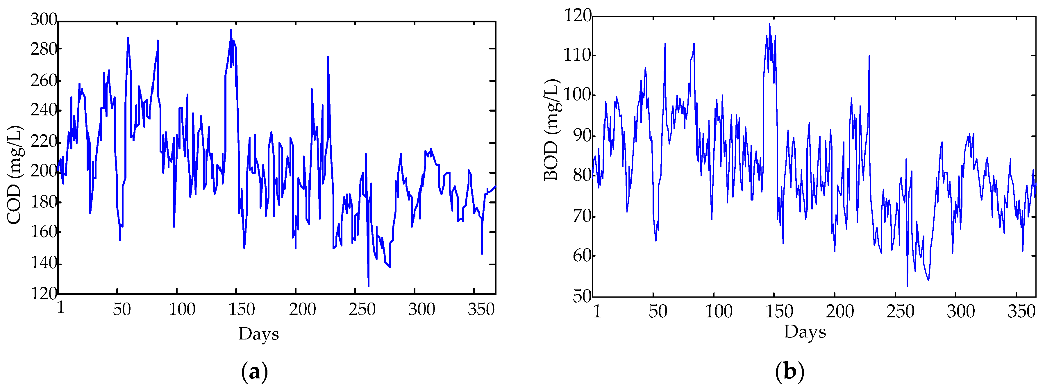
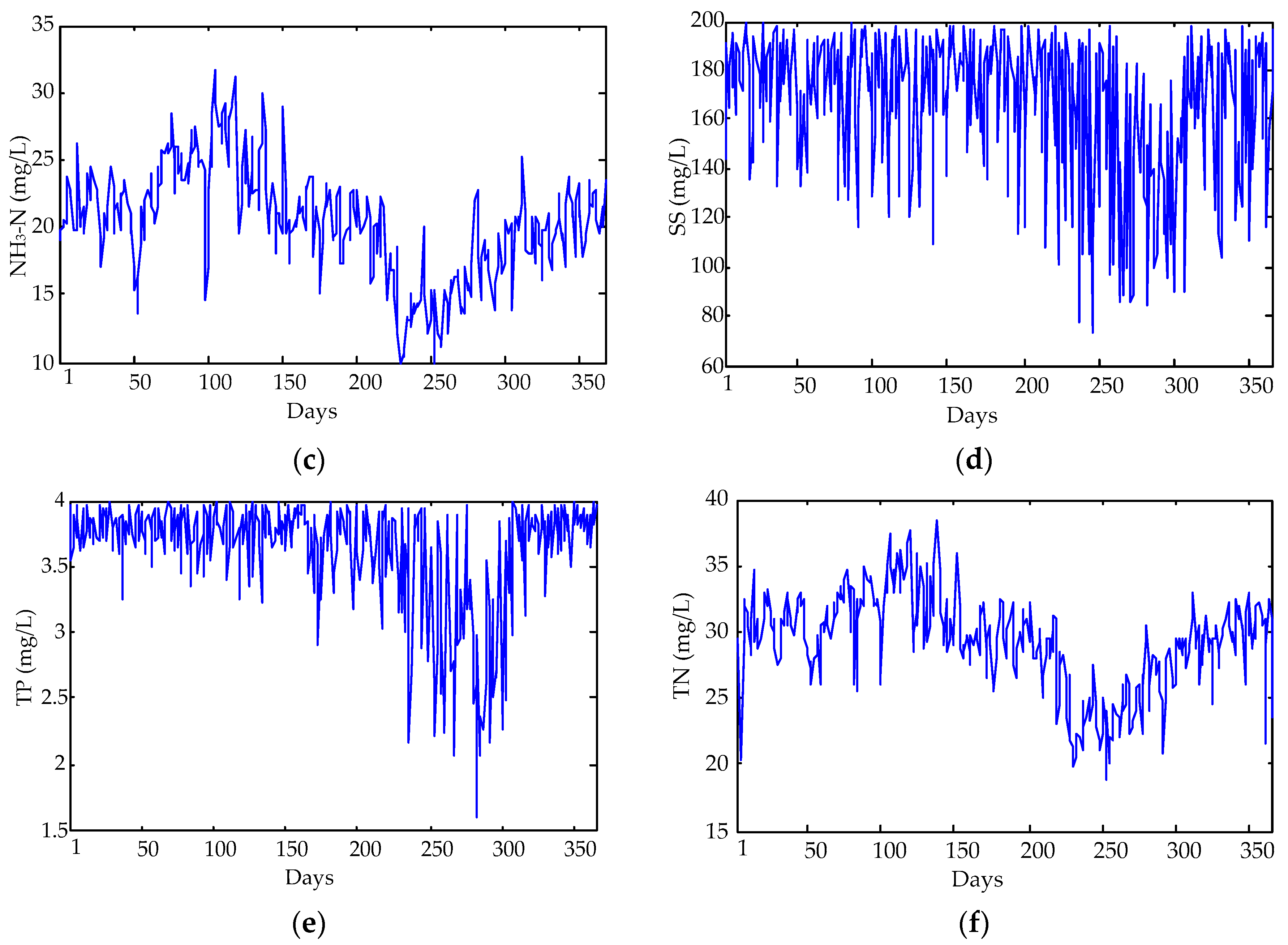
The original data for sewage treatment monitoring during 1/1/2015–31/12/2015 are used in this study, and include COD (mg/L), BOD (mg/L), NH3-N (mg/L), SS (mg/L), TP (mg/L), and TN (mg/L). There are a total of 365 × 6 samples, which are divided into two categories, i.e., the former 300 × 6 samples for model training, and the rest (65 × 6 samples) for model testing. Each index’s daily mean values nonlinear change trend is shown in Figure 2.
Next, the statistical properties, including the maximum, minimum, mean, and standard deviation (SD), are calculated for further analysis to get a deeper understanding. Table 1 illustrates the statistical properties of COD and BOD in respect of the divided training and testing sets, and Table 2 details the statistical properties of the variables. According to Table 1, the training and testing sets have different statistical properties, so it can better explain the performance of the predicted results. From Table 2 and Figure 2, it can be found that the data has the characteristics of violent fluctuation, and the magnitudes of the variables clearly display a big difference. In fact, the effect of the variables with a large magnitude on the modeling is larger than the one with a small magnitude, and thus it is not appropriate to directly take the data to establish the model [55]. Thus, all the data are normalized to (0, 1) with the same magnitude to eliminate the influence of the dimension among variables before applying them in the experiments.
Figure 2 and Table 1, Table 2 and Table 3 indicate that each index value of inlet water quality is outside the standard range. Hence, it is important for the sewage treatment to build a reasonable process plan for disposing of the inlet wastewater, to meet the nation discharge standard of sewage. Establishing a reliable forecasting model not only helps to adjust the performance parameters, such as the balance of carbon source, aeration rates, and reflux ratio, but also to minimize the operation costs and energy consumption.
3.2. Process of Sewage Treatment
A traditional Anaerobic/Anoxic/Oxic (A/A/O) process is applied to treat domestic sewage in WWTP, which exhibits a good performance for nutrient removal. However, the performance parameter of any WWTP must be modified according to the actual condition of the A/A/O process. Otherwise, the efficiency of the WWTP cannot meet the initial design properties and it may result in serious energy waste [56]. Better control of a WWTP can be achieved by developing robust models for forecasting the plant performance based on the past observation of certain water quality factors. This study uses a combination of the KPCA and ELM to extract the principal components from past observation data for forecasting inlet COD and BOD concentration, which helps to adjust the performance parameters, such as the balance of carbon source, aeration rates, and reflux ratio. The A/A/O process flow is shown in Figure 3.
3.3. Experimental Design
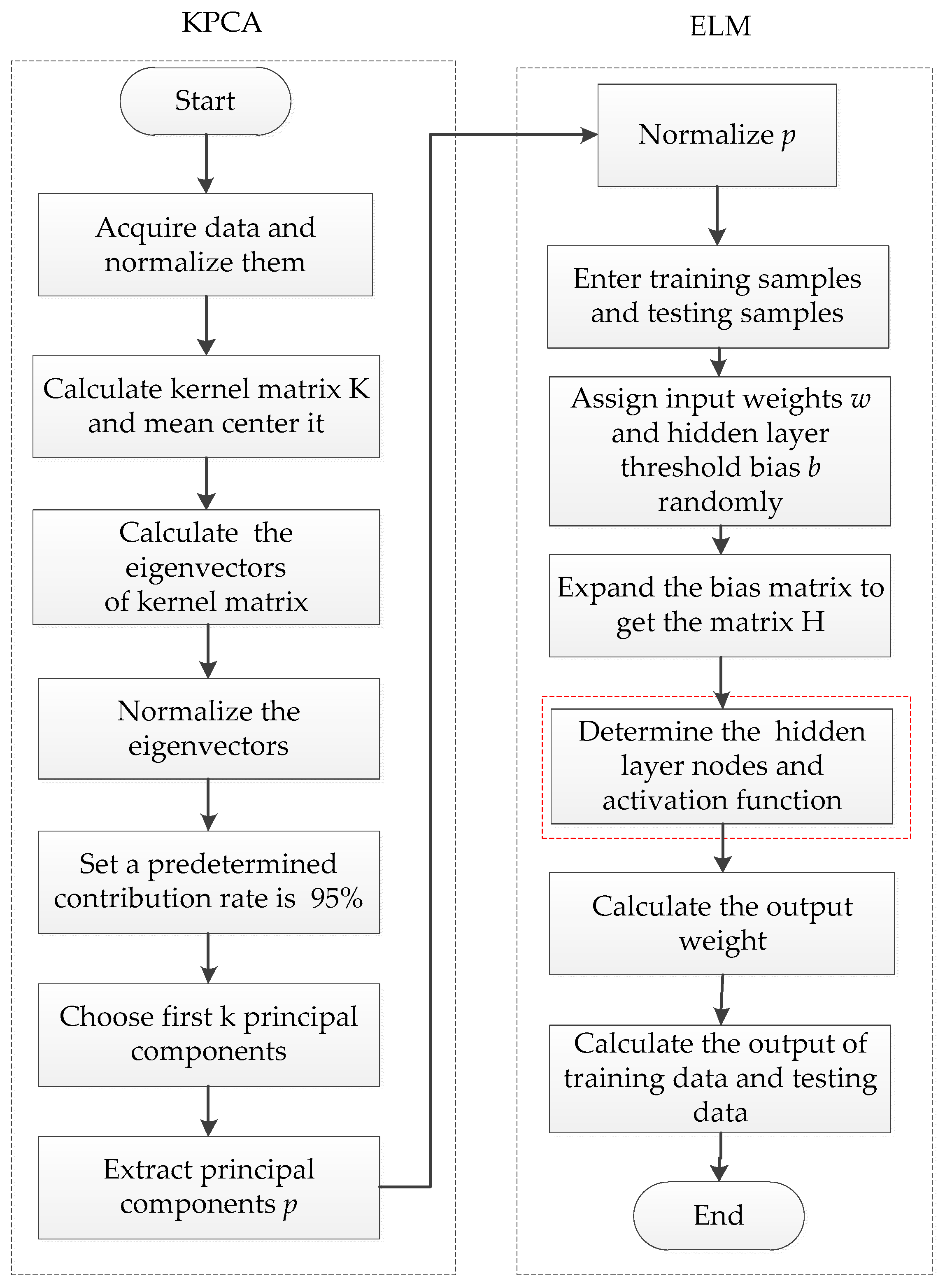
The experimental design processing of the KPCA-ELM model is shown in Figure 4.
The KPCA experimental influences related to choosing the first p eigenvectors will have a direct effect, specifically:
- (a)
- Choose p eigenvectors by trial and error, which corresponds to the first p biggest eigenvalues to form the sub-eigenspace.
- (b)
- As shown in Equation (6), if the starting p eigenvalues are over 95% of the total eigenvalues, then the information can be presented by p principle components in practical applications.
The principle components are extracted by the KPCA algorithm as the input of the ELM. In the ELM experimental section, there are the two important parameters (hidden layer nodes and activation function). The specific operation of the selection steps is established as follows:
- (a)
- The trial and error method is used to select the optimal activation function with root mean square error (RMSE) as the criteria.
- (b)
- The sigmoid function is selected as the activation function [57], and the sigmoid function is expressed as follows:
3.4. Assessing the Performance of the Forecasting Model
Bulleted lists look like this: To assess the performance of the proposed model, three criteria, mean absolute error (MAE), mean absolute percentage error (MAPE), and root mean square error (RMSE), are applied in this paper.
Mean absolute error (MAE)
Mean absolute percentage error (MAPE)
Root mean square error (RMSE)
where y represents the observed values, represents the forecasting values, and N is the length of the output data series.
4. Results and Discussion
4.1. Assessing the Performance of the Forecasting Model
The COD, BOD, NH3-N, SS, TP, and TN provided by the sewage treatment plant are used as the input parameters of the water quality forecasting. After the KPCA processing, the principal components are extracted. As shown in Figure 5, the contribution rate of the three principal components is up to 98.20%. Therefore, one can employ these three principal components as the input in the next forecasting process.
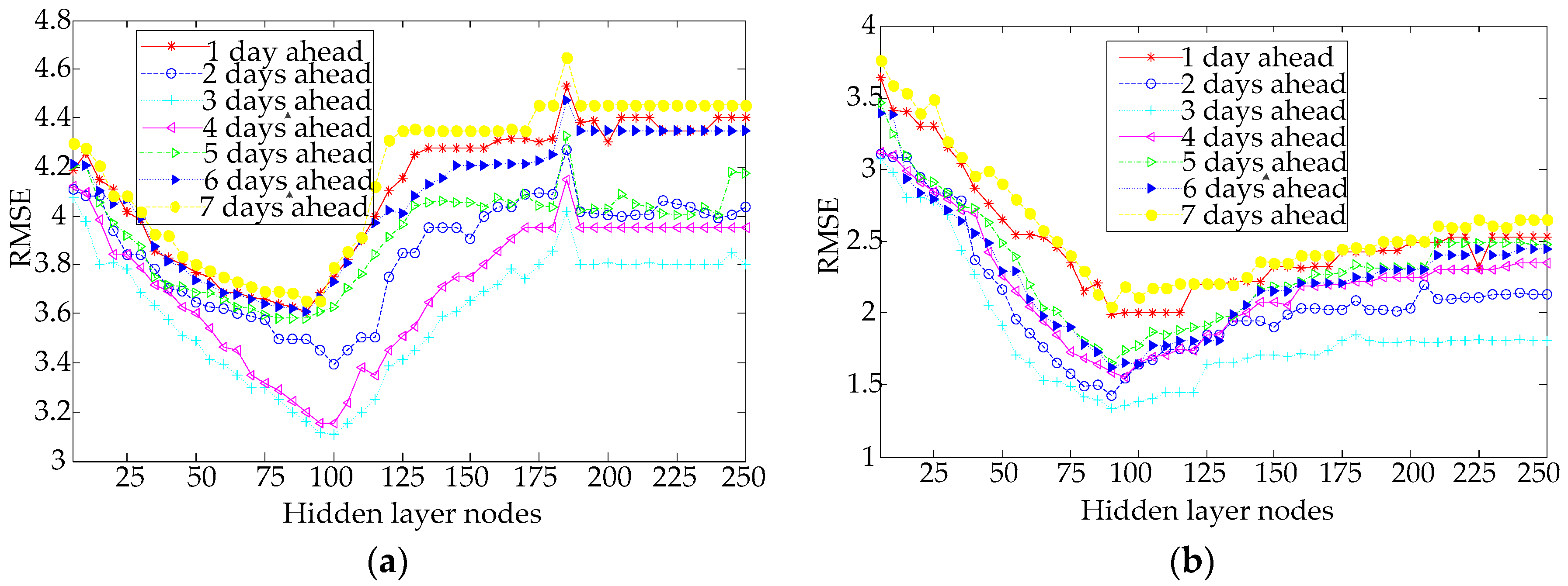
The parameters in the algorithms are determined by trial and error. In this study, the hidden layer nodes for the model are gradually increased from 5 to 250 with the interval 5. In addition, the model forecasts the values of the COD and BOD concentrations at time t using the three principal components in the input structure with different time lags (up to seven prior days) [58].
In this paper, the RMSE, defined as Equation (18), is used to evaluate the regression accuracy for forecasting inlet COD and BOD under the different number of hidden layer nodes and different time lags, as in Figure 6a,b, respectively.
Figure 6a demonstrates that the RMSE values of the COD forecasting with an increasing the number of hidden layer nodes decreased and then increased for the different lags. The best performance of the COD forecasting is achieve when the number of the hidden layer nodes is 100 with three days ahead, and the lowest RMSE value is 3.108. As shown in Figure 6b, for the proposed model to forecast BOD with an increasing number of hidden layer nodes, the RMSE values are decreased, and then gradually stabilized. The lowest RMSE value of the BOD is 1.340 with 90 hidden layer nodes and three days ahead.
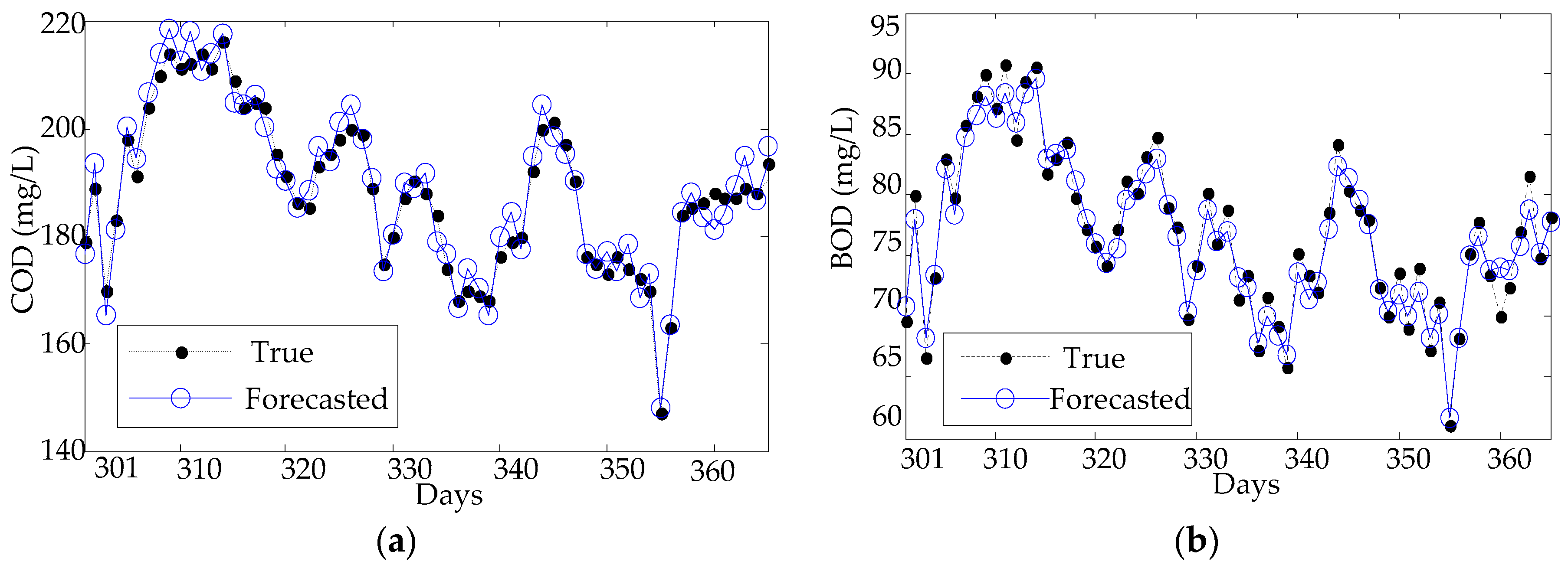
Under the best performance structure, the comparison between the forecasting value and true value of inlet COD and BOD concentration is as seen in Figure 6.
From Figure 7, one can find that the forecasting results of the KPCA-ELM can follow the changes in the testing data successfully, and the forecasting curve is consistent with the testing curve, both for the COD and the BOD. The model has a sufficient ability to forecast peak data both the forecasting value of inlet COD and BOD concentration. The experimental results show that the proposed approach has some good attributes, e.g., a superior accuracy and higher stability, which can meet the requirements of the water quality forecasting of wastewater treatment.
4.2. Comparisons
To validate the prediction capacity of the proposed model, three methods are compared with the KPCA-ELM model using the same dataset: PCA-ELM, ELM, and BPNN. A comparison of the dimension reduction ability of the PCA method and KPCA method can be seen in Table 4. It shows that the PCA accumulation is only 89.923%, and the KPCA accumulation is up to 98.200% for three principal components extraction (i = 3). It illustrates that the KPCA retains much more information than that of the PCA with the same principal components.
The parameters of the PCA-ELM model, ELM model, and BPNN model of the inlet COD and BOD forecasting are determined by trial and error. For the BPNN model, the hidden layer nodes are trained by the empirical formula (, where nl represents the hidden nodes, q represents input layer nodes, s represents the output layer nodes, and is equal to [0, 10]). The comparison model settings with the optimal structures are detailed in Table 5.
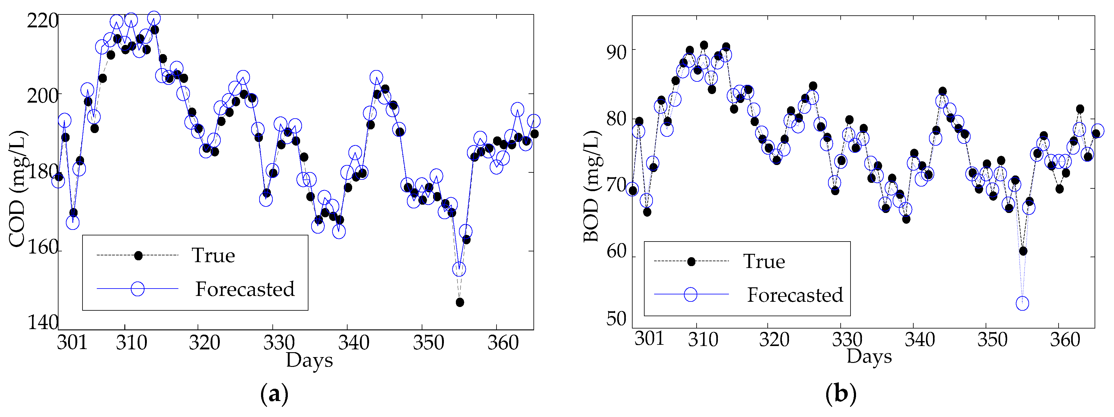
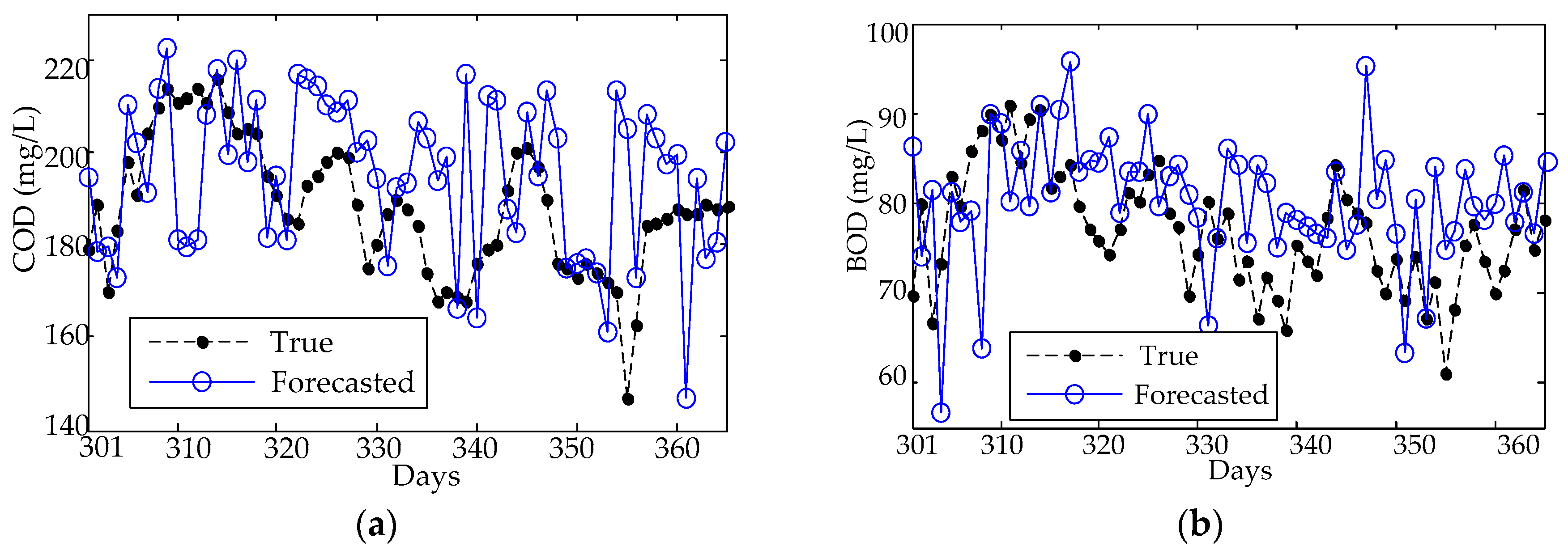
For comparison, the forecasting results of the PCA-ELM model, ELM model, and BPNN model with the best performance structures are shown in Figure 8, Figure 9 and Figure 10, respectively.
From Figure 8, one can find that the forecasting results of the PCA-ELM can follow the trends of the testing data, but fail the peak data (the 55th day) in terms of both the forecasting values of inlet COD and BOD concentration. To explore the uncertainty from different nodes of KPCA-ELM and PCA-ELM, RMSE, MAE, and MAPE variations are analyzed in each trial case. As shown in Figure 9, the forecasting results of the ELM can follow the fluctuation of the testing data, but fail the detail value of both COD and BOD concentration forecasting. The results of the BPNN model are illustrated in Figure 10, which shows the great error between the forecasted value and true value and fails to follow the fluctuation of the testing data of both COD and BOD concentration forecasting.
4.3. Statistical Analysis
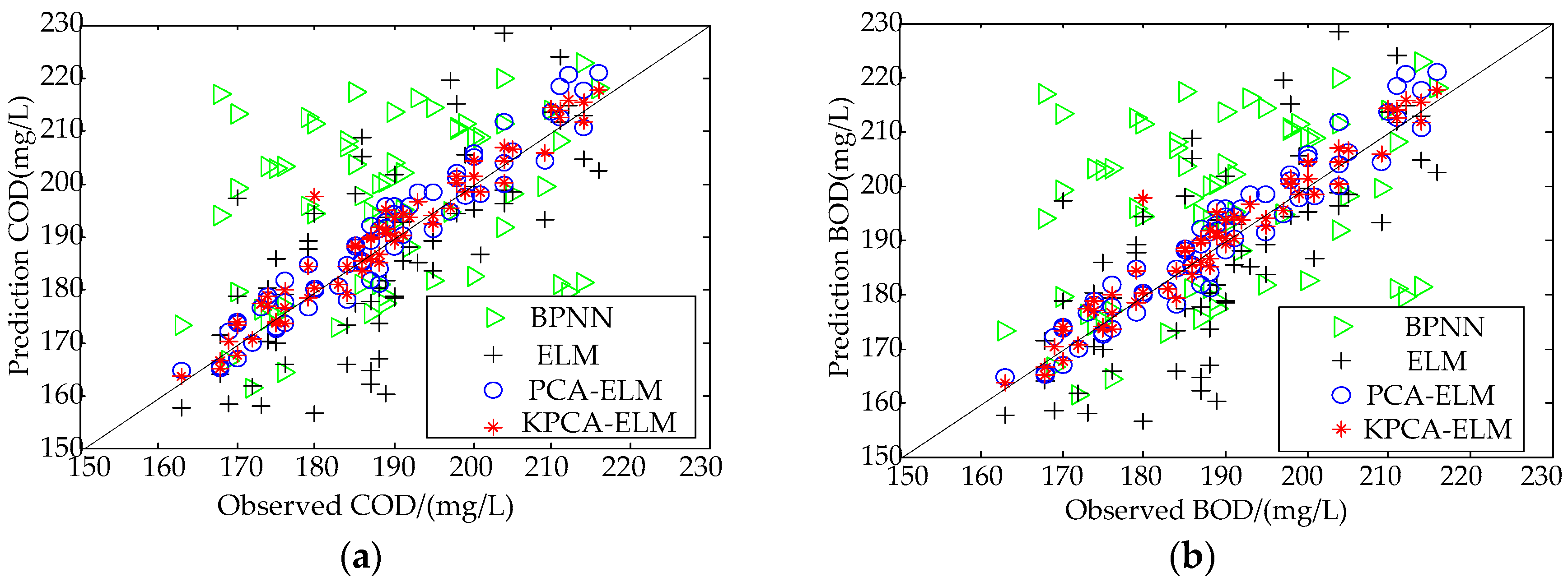
To further compare the performance and effectiveness of the models, the correlation between the predicted values of the different approaches and observed values is demonstrated in Figure 11.
As observed from Figure 11, most of the predicted values of the KPCA-ELM and PCA are closer to y = x than ELM, but a few predicted values of PCA-ELM are far away from y = x for both the COD prediction and BOD prediction. Simultaneously, the correlation coefficient of COD forecasting of the BPNN, ELM, PCA-ELM, and KPCA-ELM is equal to 0.4527, 0.7164, 0.9544, and 0.9844, respectively; and the correlation coefficient of BOD forecasting of the BPNN, ELM, PCA-ELM, and KPCA-ELM is equal to 0.5494, 0.7928, 0.9593, and 0.9864, respectively. This further illustrates the superior performance of the proposed approach.
In addition to the qualitative comparison using the forecasting results and the residual error analysis, the RMSE, MAE, and MAPE are used to quantitatively evaluate the forecasting performance among the KPCA-ELM, the PCA-ELM, and the ELM. The experimental results indicated that the KPCA-ELM model has a higher accuracy than the others for forecasting COD and BOD concentration of the inlet wastewater, with MAE values of 2.322 mg/L and 1.125 mg/L, MAPE values of 1.223% and 1.321%, and RMSE values of 3.108 and 1.340, respectively. The PCA-ELM model for forecasting COD and BOD concentration of the inlet wastewater displayed MAE values of 3.542 mg/L and 1.125 mg/L, MAPE values of 1.900% and 1.777%, and RMSE values of 4.270 and 1.710, respectively. The ELM model for forecasting COD and BOD concentration of the inlet wastewater exhibited MAE values of 9.125 mg/L and 4.399 mg/L, MAPE values of 6.234% and 6.057%, and RMSE values of 14.267 and 5.585, respectively. The BPNN model for forecasting COD and BOD concentration of the inlet wastewater had MAE values of 15.826 mg/L and 6.950 mg/L, MAPE values of 8.061% and 8.783%, and RMSE values of 20.126 and 8.817, respectively. Quantitative analysis was employed and the results are summarized in Table 6. The comparative analyses demonstrate that the proposed model has a better forecasting performance according to each of the three criteria.
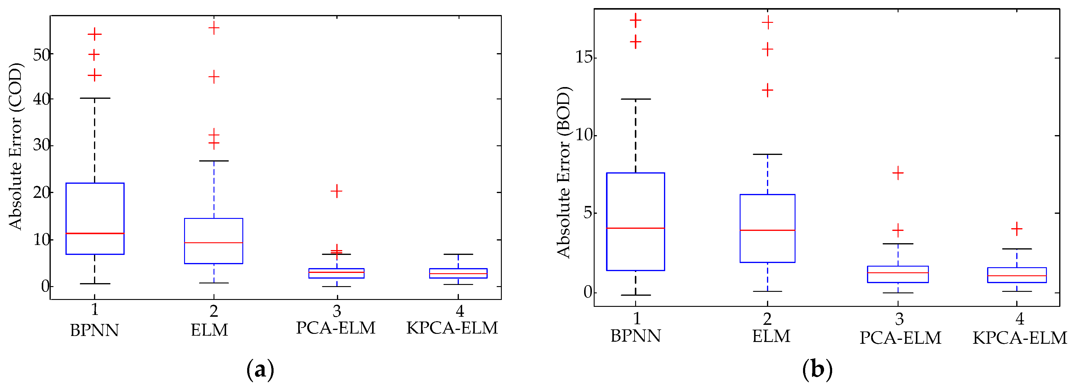
Additionally, to further validate the performance of the proposed model, an error boxplot is drawn in Figure 12. The boxplot often helps to indicate the degree of dispersion and skewedness in the data, and identifies outliers. As indicated in Figure 12, the results generated by the KPCA-ELM and the PCA-ELM are shorter than those of the ELM and BPNN when observing the length of each box entity, indicating that the distributions of the absolute error are relatively concentrated using the KPCA or the PCA. Nevertheless, the location of the entity for the KPCA-ELM is lower than the PCA-ELM, and the mean absolute error for the KPCA-ELM is the lowest. Through counting the amount of outliers of every model, the ELM has the most, followed by the PCA-ELM, and the KPCA-ELM has the least. In addition, when comparing the distance between the median and the quartiles, the situation of the KPCA-ELM is relatively symmetrical and has a basically normal distribution. Therefore, the proposed model also overwhelms the comparison models.
In terms of the comparison analysis above, all the results sufficiently illustrate that the ELM model improved by the KPCA for the feature extraction and dimension reduction (KPCA-ELM) exhibits the best forecasting performance when compared to the application of the PCA-ELM and the ELM.
The KPCA-ELM model has been constructed for forecasting the inlet water quality of sewage treatment. Combining the fast learning capacity of the ELM with the nonlinear feature extraction ability of the KPCA, the proposed model exhibits the best forecasting performance among all the peer methods. In addition, the KPCA-ELM has the same performances for both BOD and COD, demonstrating that it has better generalization abilities.
5. Conclusions
The inlet COD and BOD concentration forecasting of wastewater treatment based on KPCA and ELM is proposed in this study. The KPCA-ELM model is can be used to control parameter adjustment of the sewage treatment system by providing a data reference, which provides a convenient and economic approach to achieve better control of WWTP. The KPCA is employed for feature extraction and dimensionality reduction of the inlet wastewater quality from the sewage treatment in 2015. In each mode, the best outputs of the ELM are determined by selecting the optimal activation function and the number of hidden layer nodes. In addition, the PCA-ELM, the ELM, and the BPNN are introduced as contrast approaches. The experimental results indicate that the KPCA-ELM method has a better forecasting capacity than the peer methods for MAE, MAPE, and RMSE. Simulations results from a wastewater treatment show that the reliability and accuracy of the KPCA-ELM model outperform the PCA-ELM model, the ELM model, and the BPNN model.
In this work, it is shown that KPCA can explore higher order information of the original inputs than the PCA, and the ELM provides a better generalization performance than other popular learning algorithms and faster speeds. Thus, the presented model can be found to excel in water quality forecasting of wastewater treatment in ways that are complex, nonlinear, and uncertain.
Author Contributions
T.Y. implemented the algorithm and wrote this paper; S.Y. improved English quality; Y.B. proposed the framework of this manuscript and designed the experiments; X.G. provided the original data and relative analysis; C.L. contributed the revision of this manuscript.
Funding
This work is supported in part by the National Key Research & Development Program of China (2016YFE0205600), the Humanities and Social Science Foundation of Ministry of Education of China (17YJC630003), the Program of Chongqing Municipal Education Commission (KJZH17123), and the Research Start-Up Funds of Chongqing Technology and Business University (1756012).
Acknowledgments
The authors would like to thank precious suggestions by two anonymous reviewers and editors, which have greatly helped the improvement of the paper.
Conflicts of Interest
The authors declare no conflict of interest.
References
- Chen, H.; Teng, Y.; Wang, J. A framework of characteristics identification and source apportionment of water pollution in a river: A case study in the Jinjiang River, China. Water Sci. Technol. 2012, 65, 2071–2078. [Google Scholar] [CrossRef] [PubMed]
- Chang, C.H.; Cai, L.Y.; Lin, T.F.; Chung, C.L.; Linden, L.; Burch, M. Assessment of the impacts of climate change on the water quality of a small deep reservoir in a humid-subtropical climatic region. Water 2015, 7, 1687–1711. [Google Scholar] [CrossRef]
- Kusiak, A.; Verma, A.; Wei, X. A data-mining approach to predict influent quality. Environ. Monit. Assess. 2013, 185, 2197–2210. [Google Scholar] [CrossRef] [PubMed]
- Aminabad, M.S.; Maleki, A.; Hadi, M.; Shahmoradi, B. Application of Artificial Neural Network (ANN) for the prediction of water treatment plant influent characteristics. J. Adv. Environ. Health Res. 2014, 1, 1–12. [Google Scholar]
- Nasr, M.S.; Moustafa, M.A.E.; Seif, H.A.E.; Kobrosy, G.E. Application of Artificial Neural Network (ANN) for the prediction of EL-AGAMY wastewater treatment plant performance-EGYPT. Alex. Eng. J. 2012, 51, 37–43. [Google Scholar] [CrossRef]
- Maleki, A.; Nasseri, S.; Aminabad, M.S.; Hadi, M. Comparison of ARIMA and NNAR models for forecasting water treatment plant’s influent characteristics. KSCE J. Civ. Eng. 2018, 1–13. [Google Scholar] [CrossRef]
- Wang, X.; Ratnaweera, H.; Holm, J.A.; Olsbu, V. Statistical monitoring and dynamic simulation of a wastewater treatment plant: A combined approach to achieve model predictive control. J. Environ. Manag. 2017, 193, 1–7. [Google Scholar] [CrossRef] [PubMed]
- Akpan, V.A.; Osakwe, R.A.O. Online prediction of influent characteristics for wastewater treatment plants management using adaptive recursive NNARMAX model. Mol. Nutr. Food Res. 2014, 52 (Suppl. 2), S208–S219. [Google Scholar]
- Liu, W.; Wang, G.Y.; Fu, J.Y.; Zou, X. Water quality prediction based on improved wavelet transformation and support vector machine. Adv. Mater. Res. 2013, 726–731, 3547–3553. [Google Scholar] [CrossRef]
- Martínez-Bisbal, M.C.; Loeff, E.; Olivas, E.; Carbo, N.; Garcia-Castillo, F.J.; Lopez-Carrero, J.; Tormos, I.; Tejadillos, F.J.; Berlanga, J.G.; Martnez-Manez, R.; et al. A voltammetric electronic tongue for the quantitative analysis of quality parameters in wastewater. Electroanalysis 2017, 29, 1147–1153. [Google Scholar] [CrossRef]
- Langeveld, J.; Daal, P.V.; Schilperoort, R.; Nopens, I.; Flameling, T.; Weijers, S. Empirical sewer water quality model for generating influent data for WWTP modelling. Water 2017, 9, 491. [Google Scholar] [CrossRef]
- Srividya, M.; Mohanavalli, S.; Bhalaji, N. Behavioral modeling for mental health using machine learning algorithms. J. Med. Syst. 2018, 45, 88. [Google Scholar] [CrossRef] [PubMed]
- Cambria, E.; Gastaldo, P.; Bisio, F.; Zunino, R. An ELM-based model for affective analogical reasoning. Neurocomputing 2015, 149, 443–455. [Google Scholar] [CrossRef]
- Low, Y.; Gonzalez, J.E.; Kyrola, A.; Bickson, D.; Guestrin, C.; Hellerstein, J.M. GraphLab: A new framework for parallel machine learning. arXiv, 2010; arXiv:1408.2041. [Google Scholar]
- Domingos, P. A few useful things to know about machine learning. Commun. ACM 2012, 55, 78–87. [Google Scholar] [CrossRef]
- Rong, H.J.; Ong, Y.S.; Tan, A.H.; Zhu, Z.A. A fast pruned-extreme learning machine for classification problem. Neurocomputing 2008, 72, 359–366. [Google Scholar] [CrossRef]
- Ding, S.F.; Zhang, Y.N.; Xu, X.Z.; Lina, B. A Novel Extreme Learning Machine Based on Hybrid Kernel Function. J. Comput. 2013, 8, 2110–2117. [Google Scholar] [CrossRef]
- Deo, R.C.; Şahin, M. Application of the extreme learning machine algorithm for the prediction of monthly effective drought index in eastern Australia. Atmos. Res. 2015, 153, 512–525. [Google Scholar] [CrossRef]
- Huang, G.B.; Zhu, Q.Y.; Siew, C.K. Extreme learning machine: Theory and applications. Neurocomputing 2006, 70, 489–501. [Google Scholar] [CrossRef] [Green Version]
- Akusok, A.; Gritsenko, A.; Miche, Y.; Björk, K.M.; Nian, R.; Lauren, P.; Lendasse, A. Adding reliability to ELM forecasts by confidence intervals. Neurocomputing 2017, 219, 232–241. [Google Scholar] [CrossRef]
- Shamshirband, S.; Mohammadi, K.; Yee, P.L.; Petković, D.; Mostafaeipour, A. A comparative evaluation for identifying the suitability of extreme learning machine to predict horizontal global solar radiation. Renew. Sustain. Energy Rev. 2015, 52, 1031–1042. [Google Scholar] [CrossRef]
- Lian, C.; Zeng, Z.; Yao, W.; Tang, H. Ensemble of extreme learning machine for landslide displacement prediction based on time series analysis. Neural Comput. Appl. 2014, 24, 99–107. [Google Scholar] [CrossRef]
- Xiao, C.; Dong, Z.; Xu, Y.; Meng, K.; Zhou, X.; Zhang, X. Rational and self-adaptive evolutionary extreme learning machine for electricity price forecast. Memet. Comput. 2016, 8, 223–233. [Google Scholar] [CrossRef] [Green Version]
- Li, S.; Wang, P.; Goel, L. Short-term load forecasting by wavelet transform and evolutionary extreme learning machine. Electr. Power Syst. Res. 2015, 122, 96–103. [Google Scholar] [CrossRef]
- Barzegar, R.; Moghaddam, A.A.; Adamowski, J.; Ozga-Zielinski, B. Multi-step water quality forecasting using a boosting ensemble multi-wavelet extreme learning machine model. Stoch. Environ. Res. Risk A 2018, 32, 799–813. [Google Scholar] [CrossRef]
- Yousefi, F.; Mohammadiyan, S.; Karimi, H. Viscosity of carbon nanotube suspension using artificial neural networks with principal component analysis. Heat Mass Transf. 2016, 80, 1538–1544. [Google Scholar] [CrossRef]
- Lei, Y.; Bennamoun, M.; Hayat, M.; Guo, Y. An efficient 3D face recognition approach using local geometrical signatures. Pattern Recognit. 2014, 47, 509–524. [Google Scholar] [CrossRef]
- Bai, Y.; Wang, P.; Li, C.; Xie, J.; Wang, Y. A multi-scale relevance vector regression approach for daily urban water demand forecasting. J. Hydrol. 2014, 517, 236–245. [Google Scholar] [CrossRef]
- Gonçalves, A.M.; Alpuim, T. Water quality monitoring using cluster analysis and linear models. Environmetrics 2011, 22, 933–945. [Google Scholar] [CrossRef]
- Bai, Y.; Chen, Z.Q.; Xie, J.J.; Li, C. Daily reservoir inflow forecasting using multiscale deep feature learning with hybrid models. J. Hydrol. 2016, 532, 193–206. [Google Scholar] [CrossRef]
- Park, C.H.; Park, H. A comparison of generalized linear discriminant analysis algorithms. Pattern Recognit. 2008, 41, 1083–1097. [Google Scholar] [CrossRef] [Green Version]
- Calhoun, V.D.; Liu, J.; Adali, T. A review of group ICA for fMRI data and ICA for joint inference of imaging, genetic, and ERP data. Neuroimage 2009, 45 (Suppl. 1), 163–172. [Google Scholar] [CrossRef] [PubMed]
- Gaskin, C.J.; Happell, B. On exploratory factor analysis: A review of recent evidence, an assessment of current practice, and recommendations for future use. Int. J. Nurs. Stud. 2014, 51, 511–521. [Google Scholar] [CrossRef] [PubMed]
- Teixeira, A.R.; Tomé, A.M.; Stadlthanner, K.; Lang, E.W. KPCA denoising and the pre-image problem revisited. Digit. Signal Process. 2008, 18, 568–580. [Google Scholar] [CrossRef]
- Yu, M.D.; He, X.S.; Xi, B.D.; Gao, R.T.; Zhao, X.W.; Zhang, H.; Huang, C.H.; Tan, W. Investigating the composition characteristics of dissolved and particulate/colloidal organic matter in effluent-dominated stream using fluorescence spectroscopy combined with multivariable analysis. Environ. Sci. Pollut. Res. 2018, 25, 9132–9144. [Google Scholar] [CrossRef] [PubMed]
- Xin, X.Y.; Huang, G.H.; An, C.J.; Huang, C.; Weger, H.; Zhao, S.; Zhou, Y.; Rosendahl, S.M. Insights into the Toxicity of Triclosan to Green Microalga Chlorococcum sp. using Synchrotron-based Fourier Transform Infrared Spectromicroscopy: Biophysiological Analyses and Roles of Environmental Factors. Environ. Sci. Technol. 2018, 54, 2295–2306. [Google Scholar] [CrossRef] [PubMed]
- Abdi, H.; Williams, L.J. Principal component analysis. WIREs Comput. Stat. 2010, 2, 433–459. [Google Scholar] [CrossRef] [Green Version]
- Zhang, Y.; Ma, C. Fault diagnosis of nonlinear processes using multiscale KPCA and multiscale KPLS. Chem. Eng. Sci. 2011, 66, 64–72. [Google Scholar] [CrossRef]
- Kuang, F.; Xu, W.; Zhang, S.; Wang, Y.; Liu, K. A novel approach of KPCA and SVM for intrusion detection. J. Comput. Inf. Syst. 2012, 8, 3237–3244. [Google Scholar]
- Ma, H. Formation drillability prediction based on multi-source information fusion. J. Petrol. Sci. Eng. 2011, 78, 438–446. [Google Scholar] [CrossRef]
- Ren, F.; Wu, X.; Zhang, K.; Niu, R. Application of wavelet analysis and a particle swarm-optimized support vector machine to predict the displacement of the Shuping landslide in the Three Gorges, China. Environ. Earth Sci. 2015, 73, 4791–4804. [Google Scholar] [CrossRef]
- Jin, H.; Lee, B.M.; Lee, T.; Park, D.H. Estimation of biological oxygen demand and chemical oxygen demand for combined sewer systems using synchronous fluorescence spectra. Sensors 2010, 10, 2460–2471. [Google Scholar]
- Maruthi, Y.A.; Das, N.L.; Hossain, K.; Sarma, K.S.S.; Rawat, K.P.; Sabharwal, S. Application of electron beam technology in improving sewage water quality: An advance technique. Afr. J. Environ. Sci. Technol. 2011, 5, 545–552. [Google Scholar]
- Bhatti, Z.A.; Mahmood, Q.; Raja, I.A.; Malik, A.H.; Rashid, N.; Wu, D.L. Integrated chemical treatment of municipal wastewater using waste hydrogen peroxide and ultraviolet light. Phys. Chem. Earth A/B/C 2011, 36, 459–464. [Google Scholar] [CrossRef]
- Shao, J.D.; Rong, G.; Lee, J.M. Learning a data-dependent kernel function for KPCA-based nonlinear process monitoring. Chem. Eng. Res. Des. 2009, 87, 1471–1480. [Google Scholar] [CrossRef]
- Qian, X.; Chen, J.P.; Xiang, L.; Zhang, W.; Niu, C.C. A novel hybrid KPCA and SVM with PSO model for identifying debris flow hazard degree: A case study in Southwest China. Environ. Earth Sci. 2016, 75, 991. [Google Scholar] [CrossRef]
- Mercer, A.E.; Richman, M.B.; Leslie, L.M. Identification of severe weather outbreaks using kernel principal component analysis. Procedia Comput. Sci. 2011, 6, 231–236. [Google Scholar] [CrossRef]
- Tveit, S.; Bakr, S.A.; Lien, M.; Mannseth, T. Identification of subsurface structures using electromagnetic data and shape priors. J. Comput. Phys. 2015, 284, 505–527. [Google Scholar] [CrossRef] [Green Version]
- Zhang, Y. Enhanced statistical analysis of nonlinear processes using KPCA, KICA and SVM. Chem. Eng. Sci. 2009, 64, 801–811. [Google Scholar] [CrossRef]
- Scholkopf, B.; Alexander, S. Nonlinear component analysis as a kernel eigenvalue problem. Neural Comput. 1998, 10, 1299–1319. [Google Scholar] [CrossRef]
- Pang, Y.W.; Wang, L.; Yuan, Y. Generalized KPCA by adaptive rules in feature space. Int. J. Comput. Math. 2010, 87, 956–968. [Google Scholar] [CrossRef]
- Singh, R.; Balasundaram, S. Application of extreme learning machine method for time series analysis. Int. J. Intell. Technol. 2007, 2, 256–262. [Google Scholar]
- Yin, Z.; Qi, F.; Yang, L.S.; Deo, R.C.; Wen, X.H.; Si, J.H.; Xiao, S.C. Future projection with an extreme-learning machine and support vector regression of reference evapotranspiration in a mountainous inland watershed in North-West China. Water 2017, 9, 880. [Google Scholar] [CrossRef]
- Huang, G.B.; Li, M.B.; Chen, L.; Siew, C.K. Incremental extreme learning machine with fully complex hidden nodes. Neurocomputing 2008, 71, 576–583. [Google Scholar] [CrossRef] [Green Version]
- Jian, L.; Song, Y.Q.; Shen, S.Q.; Wang, Y.; Yin, H.Q. Adaptive least squares support vector machine prediction for blast furnace ironmaking process. ISIJ. Int. 2015, 55, 845–850. [Google Scholar] [CrossRef]
- Jiang, D.L.; Ni, G.; Jia, J.L. Performance Analysis of Anaerobic/Anoxic/Oxic (A/A/O) Process Municipal WWTPs. Adv. Mater. Res. 2012, 461, 478–481. [Google Scholar] [CrossRef]
- Zhou, Z.Y.; Xu, R.; Wu, D.C.; Wang, H.Y. Illumination correction of dyed fabrics approach using Bagging-based ensemble particle swarm optimization–extreme learning machine. Opt. Eng. 2016, 55, 93–102. [Google Scholar] [CrossRef]
- Alizadeh, M.J.; Kavianpour, M.R. Development of wavelet-ANN models to predict water quality parameters in Hilo Bay, Pacific Ocean. Mar. Pollut. Bull. 2015, 98, 171–178. [Google Scholar] [CrossRef] [PubMed]
Figure 1.
Procedure of the KPCA-ELM model.

Figure 2.
The figures of the collected water quality parameters: (a) COD; (b) BOD; (c) NH3-N; (d) SS; (e) TP; (f) TN.
Figure 2.
The figures of the collected water quality parameters: (a) COD; (b) BOD; (c) NH3-N; (d) SS; (e) TP; (f) TN.


Figure 3.
Anaerobic/Anoxic/Oxic process flow diagram.

Figure 4.
Experimental design processing.

Figure 5.
Extracted principal component by KPCA.

Figure 6.
The RMSE forecasting values under different hidden layer nodes and different time lags; (a) COD and (b) BOD.
Figure 6.
The RMSE forecasting values under different hidden layer nodes and different time lags; (a) COD and (b) BOD.

Figure 7.
Forecasting results using KPCA-ELM: (a) COD and (b) BOD.

Figure 8.
Forecasting results of the PCA-ELM model: (a) COD and (b) BOD.

Figure 9.
Forecasting results of the ELM model: (a) COD and (b) BOD.

Figure 10.
Forecasting results of the BPNN model: (a) COD and (b) BOD.

Figure 11.
Correlogram analysis of the predicted and observed values of comparison models: (a) COD and (b) BOD.
Figure 11.
Correlogram analysis of the predicted and observed values of comparison models: (a) COD and (b) BOD.

Figure 12.
Comparisons of the boxplot using different models: (a) COD and (b) BOD.


Table 1.
Statistical properties of COD and BOD in terms of divided training and testing sets.
| Set | Maximum | Minimum | Mean | SD |
|---|---|---|---|---|
| Train | 293 | 125 | 204.967 | 33.339 |
| Test | 216 | 147 | 188.2 | 14.271 |
| Train | 118 | 52.6 | 82.796 | 12.945 |
| Test | 90.8 | 61 | 79.978 | 6.613 |
Table 2.
Statistical properties of the variables.
| Pattern | No. | Variable | Maximum | Minimum | Mean | SD |
|---|---|---|---|---|---|---|
| Input | 1 | COD | 293 | 125 | 201.980 | 31.479 |
| 2 | BOD | 118 | 52.6 | 81.760 | 12.260 | |
| 3 | NH3-N | 31.6 | 10 | 20.348 | 4.093 | |
| 4 | SS | 199 | 74 | 166.5 | 29.143 | |
| 5 | TP | 3.99 | 1.59 | 3.619 | 0.423 | |
| 6 | TN | 38.4 | 18.9 | 29.248 | 3.582 | |
| Output | 1 | COD | 293 | 125 | 201.980 | 31.479 |
| 2 | BOD | 118 | 52.6 | 81.760 | 12.260 |
Table 3.
The comprehensive wastewater discharge standard (GB8978—2002).
| Assessment Factor | Unit | Judgment | Classes | |||
|---|---|---|---|---|---|---|
| I | II | III | ||||
| A | B | |||||
| COD | mg/L | ≤ | 50 | 60 | 100 | 120 |
| BOD | mg/L | ≤ | 10 | 20 | 30 | 60 |
| NH3-N | mg/L | ≤ | 5 | 8 | 25 | - |
| SS | mg/L | ≤ | 10 | 20 | 30 | 50 |
| TN | mg/L | ≤ | 15 | 20 | - | - |
| TP | mg/L | ≤ | 0.5 | 1 | 3 | 5 |
Table 4.
Comparison of the PCA and the KPCA of the principal components extraction.
| Component | PCA Accumulation % | KPCA Accumulation % |
|---|---|---|
| 1 | 54.300 | 80.487 |
| 2 | 73.313 | 90.573 |
| 3 | 89.923 | 98.200 |
Table 5.
Optimal structures of the comparison models.
| Model | Modeling Setting | |
|---|---|---|
| COD | BOD | |
| PCA-ELM | Input = 3, hidden = 85, output = 1, layer = 1, activation function: Sigmoid, time lags: two days ahead | Input = 3, hidden = 75, output = 1, layer = 1, activation function: Sigmoid, time lags: three days ahead |
| ELM | Input = 6, hidden = 80, output = 1, layer = 1, activation function: Sigmoid, time lags: four days ahead | Input = 6, hidden = 80, output = 1, layer = 1, activation function: Sigmoid, time lags: three days ahead |
| BPNN | Input = 6, hidden = 10, Output = 1, layers = 3, training: Trainlm, hidden transfer: Log-Sigmoid, output transfer: Log-Sigmoid, time lags: three days ahead | Input = 6, hidden = 10, Output = 1, layers = 3, training: Trainlm, hidden transfer: Log-Sigmoid, output transfer: Log-Sigmoid, time lags: four days ahead |
Table 6.
Comparison results using different models.
| Model | COD | BOD | ||||
|---|---|---|---|---|---|---|
| MAE | MAPE | RMSE | MAE | MAPE | RMSE | |
| BPNN | 15.826 | 8.061 | 20.126 | 6.950 | 8.783 | 8.817 |
| ELM | 9.125 | 6.234 | 14.267 | 4.399 | 6.057 | 5.585 |
| PCA-ELM | 3.542 | 1.900 | 4.270 | 1.341 | 1.777 | 1.710 |
| KPCA-ELM | 2.322 | 1.223 | 3.108 | 1.125 | 1.321 | 1.340 |
© 2018 by the authors. Licensee MDPI, Basel, Switzerland. This article is an open access article distributed under the terms and conditions of the Creative Commons Attribution (CC BY) license (http://creativecommons.org/licenses/by/4.0/).
Share and Cite
MDPI and ACS Style
Yu, T.; Yang, S.; Bai, Y.; Gao, X.; Li, C. Inlet Water Quality Forecasting of Wastewater Treatment Based on Kernel Principal Component Analysis and an Extreme Learning Machine. Water 2018, 10, 873. https://doi.org/10.3390/w10070873
AMA Style
Yu T, Yang S, Bai Y, Gao X, Li C. Inlet Water Quality Forecasting of Wastewater Treatment Based on Kernel Principal Component Analysis and an Extreme Learning Machine. Water. 2018; 10(7):873. https://doi.org/10.3390/w10070873
Chicago/Turabian StyleYu, Tingting, Shuai Yang, Yun Bai, Xu Gao, and Chuan Li. 2018. "Inlet Water Quality Forecasting of Wastewater Treatment Based on Kernel Principal Component Analysis and an Extreme Learning Machine" Water 10, no. 7: 873. https://doi.org/10.3390/w10070873
Note that from the first issue of 2016, this journal uses article numbers instead of page numbers. See further details here.