Simulation of Rain Garden Effects in Urbanized Area Based on Mike Flood

Abstract

An urban storm and surface water pollution model (MIKE FLOOD) was used to assess the impact of rain gardens on water quantity and quality for an urban area in Xi’an. After the rain garden measures were added, the results show that: (1) In the case where the total proportion of rain gardens was 2%, the overflow reduction rate was 6.74% to 65.23%, the number of overflow points reduction rate was 1.79% to 65.63%, the overload pipes reduction rate was 0% to 11.15%, the runoff reduction rate was 1.93% to 9.69%; (2) Under different rainfall conditions, the load reduction rate of suspended solids (SS), chemical oxygen demand (COD), total nitrogen (TN), and total phosphorus (TP) were 2.36% to 30.35%, 2.37% to 30.11%, 2.34% to 30.08%, and 2.32% to 31.35%, respectively; (3) The submersion ranges of different submerged depths and submerged durations were reduced by 0.30% to 64.18% and 7.12% to 100%, respectively. The statistics of the automatic modeling and intelligent analysis system (AMIAS) showed that the rain garden regulation range of the waterlogging risk area was 0.78% to 100%. The rain garden has a good control effect on urban storm runoff in terms of water volume and water quality, but as the rainfall recurrence interval increases, the control effect will decrease.

1. Introduction

With the acceleration of urbanization intensifying intrinsic risk, serious runoff pollution has become increasingly prominent, and the most direct impact has been the change in urban land-use types, which has resulted in the area of permeable subsurface becoming smaller and smaller and has also changed the hydrological mechanisms of cities [1]. The increase of impervious land surface leads to increased runoff, advanced flood peak arrival time, a large loss of rainwater resources, and an increased risk of waterlogging [2,3]. Many pollutants of runoff enter the water through the urban drainage system, which endanger the safety of the ecosystem. At present, Low Impact Development (LID) is a new strategy for international urban water environment protection and development of storm water management. With the characteristics of high elasticity, multi-functionality, source control, and natural effects, the main measures of the LID model include rain garden, bio-retention, green roof, and permeable pavement [4]. LID is based on the principle of simulating the natural hydrological conditions, adopting the concept of source control to realize rainwater control and utilization. It plays an important role in mitigating and governing the frequent occurrence of waterlogging and non-point source pollution caused by urban heavy rain. LID technology regulates runoff from the source, and can reduce runoff and reduce runoff pollution load compared with traditional rain flood control measures. Rain garden has also been known as a biological retention pool. It is an important regulatory measure in LID. It uses the chemical, biological, and physical properties of plants, microorganisms and soils to remove pollutants, thereby achieving urban storm water runoff and water quality regulation targets [5]. Real-world data is needed to calibrate and validate LID simulations.

At present, the most commonly used simulation softwares for LID are SWMM [6], MIKE URBAN [7], InfoWorks-ICM [8], SCS, HydroCAD and so on [9]. From the perspective of the simulation in different conditions of the region and the feasibility of LID measures, MIKE URBAN has the characteristics of fully simulating the process of runoff and confluence of single or continuous rainfall, accurately simulating the accumulation and migration process of various typical pollutants on different underlying surfaces of cities, and fully integrating with the simulated environment of GIS. This software is more suitable for simulation analysis of different land use scenarios and LID measures. The software has been used to implement the simulation of LID control measures for runoff, peak flow, and runoff pollutants [10]. At present, most of the research in China on the effectiveness of LID measures has been evaluated using the open source SWMM model. However, the MIKE series is able to fully simulate urban storm water and non-point source pollution and has rarely been used for the simulation of large areas. The objectives of this work are: (i) To establish a MIKE FLOOD model in the research area based on the existing pipe network system and measured data; (ii) To quantify the influence of rain gardens on urban rainfall runoff and pollutants through the results of the 1D rainwater pipe network and 2D surface, submerged under different rainfall recurrence intervals; and (iii) To offer waterlogging risk assessment of the study area and further evaluate the impact of urban storm on urban areas by the automatic modeling and intelligent analysis system (AMIAS),which utilizes the MIKE FLOOD calculation result file and analyzes the waterlogging risk level assessment map for the entire area or selected area based on the defined risk level, taking into account the water depth and the duration of the accumulated water.

2. Materials and Methods

2.1. Overview of Study Area

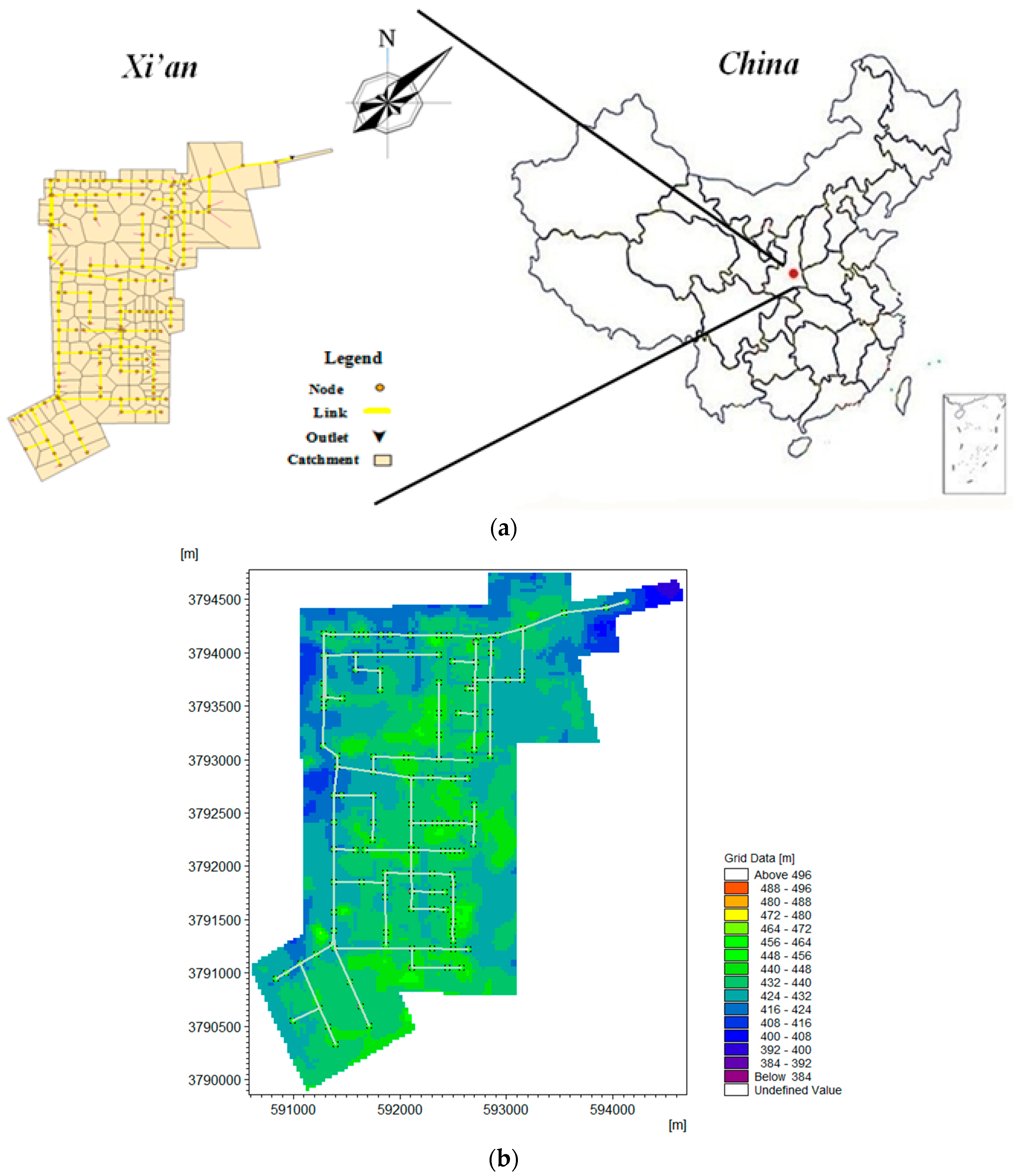
The area of Xiying Road–Chanhe River in Xi’an City was selected as the study area, with an area of approximately 8.02 km². This area belongs to the warm temperate semi-humid monsoon climate zone, with many northeast winds in winter and southwest winds in summer. The rainfall is moderate, and the average annual rainfall is 507–720 mm. Xi’an with the number of 741.14 million resident populations is a mega-city and the study area belongs to a non-central city area in Xi’an. Taking into account the nature of the study area, town types, topographical features, and climatic characteristics, the designed recurrence period of the rainwater drainage system in the study area is two years. The research area was bordered by city streets within the area shown in Figure 1.

2.2. Establishment of Study Area Model

According to the urban planning map and storm water network map of the study area from Xi’an Municipal Engineering Design and Research Institute, MIKE URBAN was used to establish a one-dimensional drainage network model for the study area. The study area is bordered by independent drainage zones and was divided into 130 sub-catchment areas. The Tyson polygon method was used in the MIKE model to divide the catchment area automatically. The drainage pipe network system in the model had 139 pipelines. The pipelines were all reinforced concrete round pipes with diameters of 500–2500 mm. There were 132 inspection well nodes, one of which entered the Chanhe River. The results are shown in Figure 1a as a 1D drainage diagram.

The first step in creating a two-dimensional surface flow model is to mesh the ground elevation model. The DEM whose source is the Geospatial Data Cloud is the Digital Elevation Model with a resolution of 1:1000. The overall terrain of the area is inclined from south to north and the site is relatively flat. This study is based on the MIKE FLOOD platform, coupling only the one-dimensional drainage network model (MIKE URBAN) and the two-dimensional surface flow model (MIKE 21). The specific coupling model generated is shown in Figure 1b.

2.3. Parameters of Model

2.3.1. Sensitivity Analysis of Model Parameters

The MIKE URBAN parameters setting of the hydrodynamic model of the pipe network determines the accuracy of the model simulation. The Morris screening method was used to analyze the hydrological hydraulic parameters and water quality parameters of the study area [11]. The sensitivities of model parameters were analyzed based on the model results with different parameters. For the total runoff, the sensitivity of the four hydrological-hydraulic parameters is ranked as follows: hydrological reduction factor > imperviousness > initial loss > mean surface velocity. Among them, the hydrological reduction factor is a high-sensitivity parameter for the total amount of runoff; imperviousness is a sensitive parameter; initial loss and mean surface velocity are insensitive parameters. For peak flow rate, the hydrological reduction factor and the imperviousness are all highly sensitive parameters, and the initial loss and the mean surface velocity are still insensitive parameters. The sensitivities of the two water quality parameters are ranked as: decay constant > dispersion factor. The decay constant is a sensitive parameter, and the dispersion factor is an insensitive parameter [12]. Based on the above analysis results, each parameter of hydraulic and water quality can be optimized and adjusted, which can greatly reduce the workload of model parameter calibration and verification.

2.3.2. Parameter Determination

This simulation takes the recommended value of the runoff coefficient given in the outdoor drainage design specifications (GB50014–2006) issued by the ministry of housing and urban-rural development in China. The empirical values determined by the types of ground cover are generally used. The area of various types of land use over the entire catchment area is calculated using the weighted average method to calculate the average runoff coefficient of the entire area. Because of the infiltration capacity and speed of the soil, the impermeability rate will change during the simulation.

The monitoring water quality indexes are suspended solids (SS), chemical oxygen demand (COD), total nitrogen (TN), and total phosphorus (TP) at each monitoring point in the study area. These parameters are measured in accordance with national standards and the data from the mean of multiple rainfall events. The samples were taken through sonders and then analyzed by ourselves. Of the pollutants in the underlying surface of the study area, SS, COD, TN, and TP in the living area were 702.27 mg/L, 497.89 mg/L, 24.29 mg/L, and 2.34 mg/L, respectively. SS, COD, TN, and TP in the commercial area were 740.45 mg/L, 527.48 mg/L, 26.04 mg/L, and 2.67 mg/L, respectively. The SS, COD, TN, and TP in the industrial area were 779.84 mg/L, 571.98 mg/L, 28.03 mg/L, and 3.14 mg/L, respectively. The SS, COD, TN, and TP in the traffic area were 1401.48 mg/L, 812.47 mg/L, 50.01 mg/L, and 5.37 mg/L, respectively.

Based on the sub-catchment areas, the model uses the Rainfall-Runoff model to calculate the runoff volume and the Time-Area curve method which is used for the confluence calculation. The tube-flow calculation uses the motion Dynamic Wave method. The cumulative and scour functions of runoff pollutants in the study area are selected as the exponential functions.

2.3.3. Parameter Calibration

Combined with the results of the sensitivity analysis, the hydraulic and water quality parameters of the model were calibrated. The model calibration is based on the following principle: Since the change in water quality changes with the change in water quantity, the water quantity parameter is first determined, and then the water quality parameter is determined [7].

In the process of parameter calibration of this study, the correlation coefficient squared (R²) and Nash–Sutcliffe efficiency coefficient (E_NS) were selected to evaluate the simulation results of the model [13]. Among them, E_NS is an index used to evaluate the model simulation accuracy. The specific formula is:

$$E_{NS}=1-\frac{{{\displaystyle \sum }}_{i=1}^n{\left(y_i-y_{i0}\right)}^2}{{{\displaystyle \sum }}_{i=1}^n{\left(y_i-y_p\right)}^2}$$

where, $E_{NS}$ is the Nash–Sutcliffe Efficiency Coefficient; $y_i$ is the measured value; $y_{i0}$ is the simulated value; $y_p$ is the mean of the measured value; and $n$ is the data sequence length. $E_{NS}$ is between −∞ and 1. When $E_{NS}$ is less than 0, the simulation accuracy is poor. A large $E_{NS}$ indicates that the simulation results are robust.

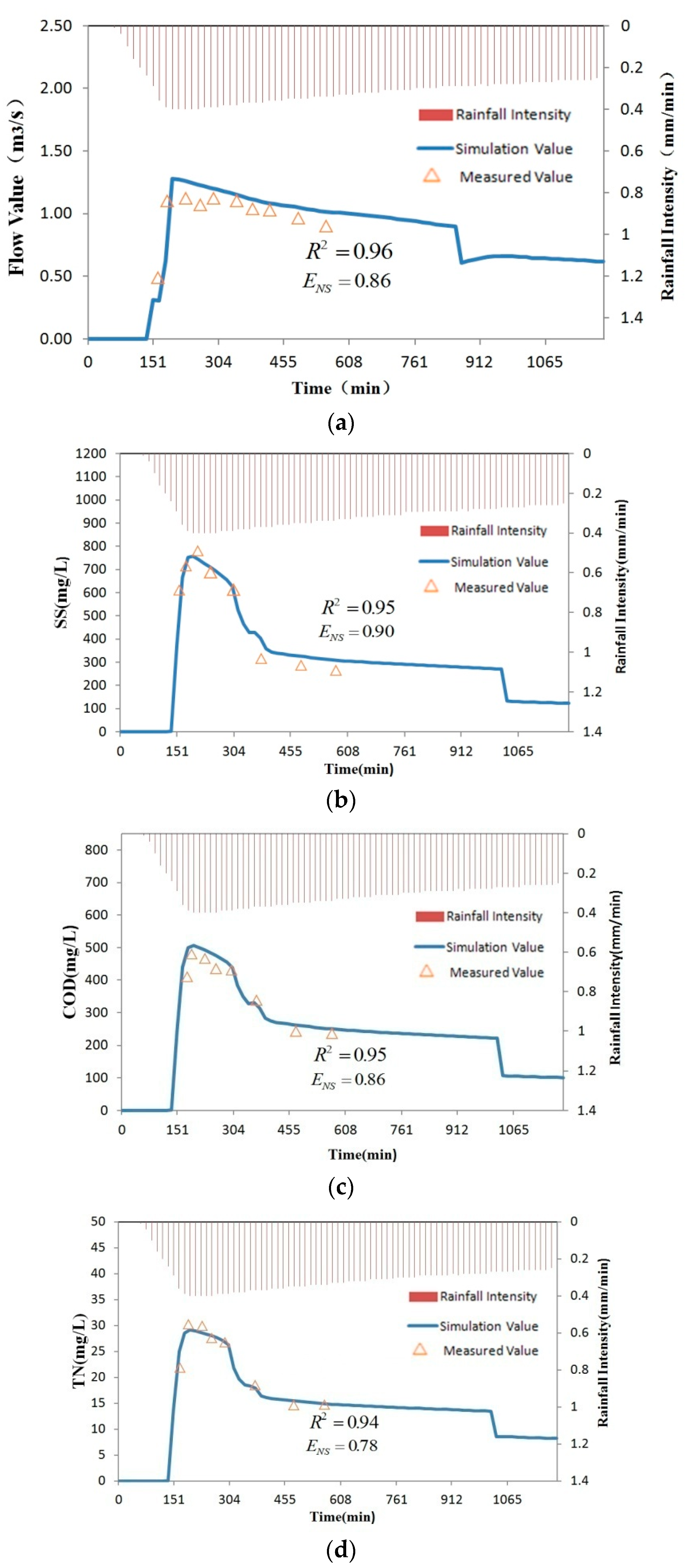
The meteorological data 13 June 2014 event rainfall was obtained from the automatic weather station using a tipping bucket rain gauge set up by us. The actual monitoring data of the total export of the study area were used to determine the relevant parameters of the model’s water quantity and water quality. The rainfall is about 23.56 mm, and it is estimated that the recurrence interval of this rainfall is nearly one year. The simulation results of the process of export flow in the study area and the concentration process of the four main pollutants were compared with the measured data in Figure 2a–e.

From Figure 2a–e, the calibration results of MIKE URBAN are well fitted with measured values. Based on the monitored flow and pollutant process data, the E_NS value of the flow rate was 0.86, and the correlation coefficient R² was 0.96. The minimum of E_NS value of the pollutant index was 0.78, and R² was higher than 0.93. The calibration results of the water volume and water quality in the study area are shown in

Table 1. Parameters of calibration results of the model.

Water Quantity	MIKE URBAN			MIKE 21			MIKE FLOOD
	MSV	HRF	Initial Loss	ISE	Flooding Depth	Drying Depth	Max Flow	Inlet Area	Discharge Coef.
	0.3 m/s	0.9	0.0006	0	0.003	0.002	1.0	0.16	0.61
Water quality				SS	COD		TN	TP
	Type			Dissolved	Suspended		Total	Total
	Initial condition			0.002	0.002		0.001	0.002
	Decay constant			0.263	0.216		0.162	0.110
	Values for each layer mg/L	Industrial		780	572		28	3.1
		Living		702	498		24	2.3
		Traffic		1401	812		50	5.4
		Commercial		740	527		26	2.7

Note: MSV is for Mean Surface Velocity; HRF is for Hydrological Reduction Factor; ISE is for Initial Surface Elevation. SS is for suspended solids; COD is for chemical oxygen demand; TN is for total nitrogen; TP is for total phosphorus.

.

2.3.4. Model validation

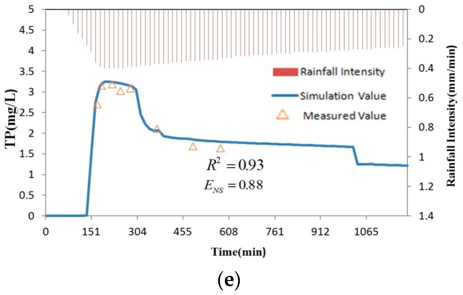
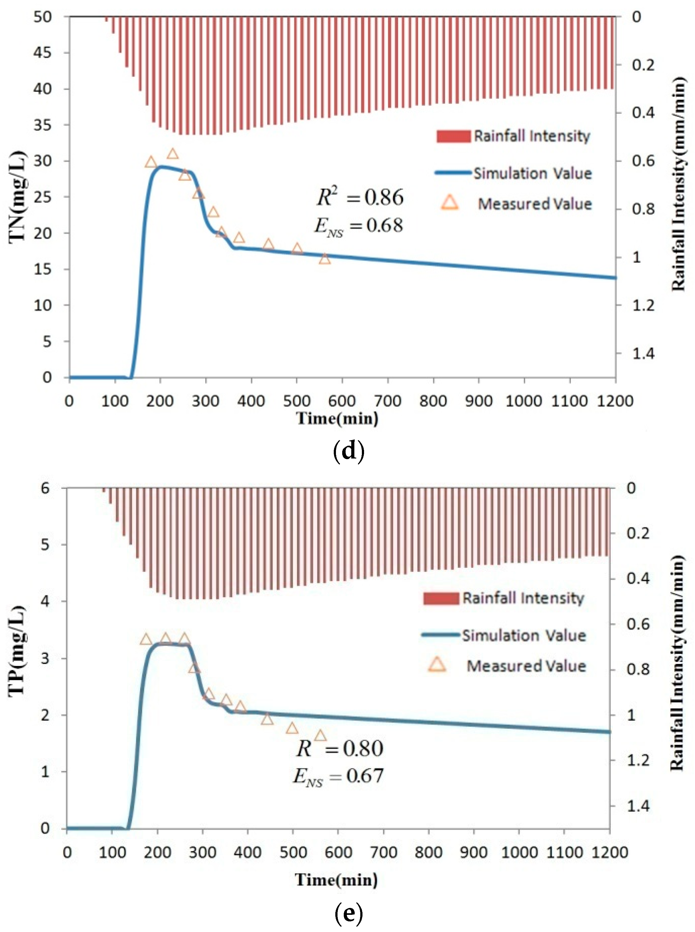
In the validation of the study area model, the square of the correlation coefficient (R²) and the Nash–Sutcliffe efficiency coefficient (E_NS) were still selected to evaluate the simulation results of the model. Using the meteorological data of 28 August 2013 and 14 October 2013 events rainfall and the actual monitoring data of the total export of the study area, the relevant parameters of the model water volume and water quality were verified separately. Taking the 14 October 2013 event as an example, the rainfall is about 28.56 mm, the recurrence interval of which is estimated to be nearly 2 years. The simulation results of the flow and the four main pollutants of the concentration process at the export of the study area are compared with the measured data, as shown in Figure 3a–e.

From Figure 3a–e, the verification results of MIKE URBAN fit well with the measured values. In the model verification results, the E_NS value of the flow rate was 0.84, and the correlation coefficient R² was 0.89; the minimum of E_NS value of the pollutant index was 0.67, and R² was higher than 0.80. For the rainfall event 2014-08-28, the E_NS value of the flow rate was 0.78, and the correlation coefficient R² was 0.81; The E_NS values of the pollutants are greater than 0.69, and R² is greater than 0.68. Therefore, these results showed that the model established in the study area has improved reliability and stability and it can be used to simulate the effects of rain garden regulation measures.

2.4. Rainfall Condition Design

We applied the determined MIKE FLOOD model to design different levels of rainfall, selected rainfall data for the same event, and compared the effects of rain garden regulation. We further analyzed the surface runoff and water quality regulation of the study area under different characteristics of rainfall events of the rain gardens and no rain gardens.

The formula for designing the rain intensity in the study area is:

$$q=\frac{2785.833 \left(1+1.658lgP\right)}{{\left(t+16.813\right)}^{0.9302}}$$

where, $q$ is the storm intensity; $P$ is the recurrence interval; and $t$ is the rainfall duration.

Domestic and foreign scholars have proposed a variety of methods to establish a short duration of rain, such as the Chicago rainfall pattern, the Huff rainfall pattern, other asymmetrical triangular rainfall patterns, and the SCS rainfall pattern. Keifer and Chu proposed the Chicago rainfall pattern, which is generally applied to short duration design rain distribution. It is based on the rain intensity formula and the rain peak coefficient of the non-constant rainfall synthesis method [14].

According to the “Description of waterlogging point distribution in pilot cities” issued by the Ministry of Housing and Urban-Rural Development Department of the People’s Republic of China (MOHURD), for the 1-year, 2-year, and 5-year rainfall recurrence intervals, it is recommended to use a short duration (2 h or 3 h) to design the rain patterns. For 10-year, 20-year, and 50-year rainfall recurrence intervals, it is recommended to use 24-h long duration rain patterns (if not, short duration rain patterns can be used). In this paper, the rain pattern was designed to use 3 h in short duration, with a time step of 5 min and a rain peak coefficient of design rainfall events of 0.4. Li et al. [15] simulated the hydrological and environmental effects at different return periods of the study area. They concluded that with the increase in rainfall intensity, the rainfall with Chicago pattern increased the parameters such as the total amount of surface runoff, total discharge peak flow, and total pollution load. The stronger the rainfall intensity, the slower these parameters increased, while the reduction rate had a downward trend. The short duration of the design of heavy rain is calculated. The rainstorm coefficient of the designed rainstorm is 0.4 based on the value of the rain peak coefficient at home and abroad. Combined with the rainstorm intensity formula, the formula to calculate the rainfall distribution process can be used directly. The rainfall distribution is calculated based on the formula of rainstorm intensity, which is calculated for (3 h) 1, 2, and 5 years, as well as long duration (24 h) of 10, 20, and 50 years of the amount of rainfall. The design rainfall is 22.14, 29.92, 40.19, 59.86, 69.24, and 82.00 mm.

2.5. Rain Garden Design

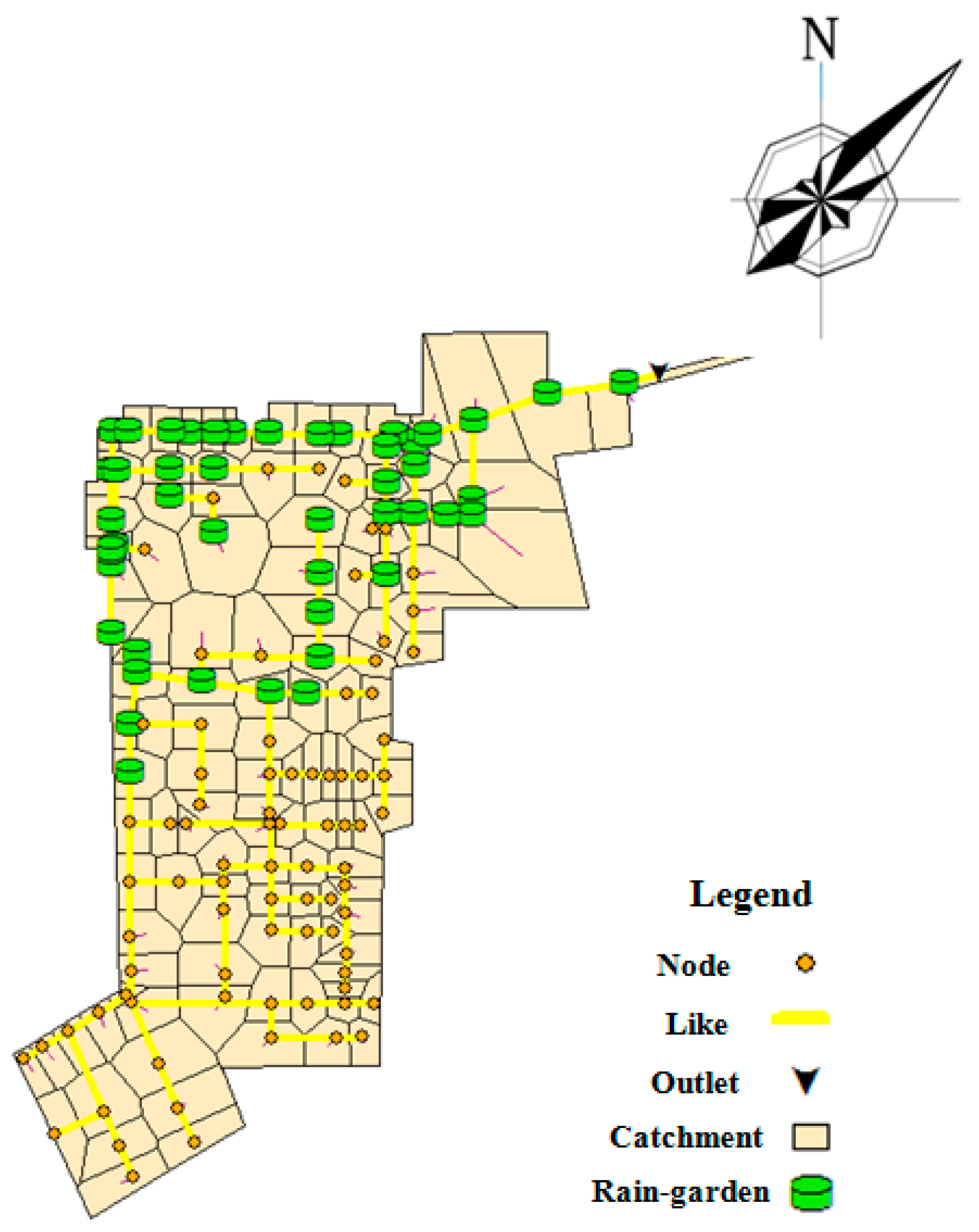
A rain garden, also known as a biological retention pool, is a combination of natural landscape construction of storm water runoff control and pollution control methods. Due to the large area of this study, considering the sudden rainfall, the rain gardens were set in a number of sub-catchments that were close to the drainage outlet of the study area and on the side of the main drainage pipe. Measuring the area of each sub-catchment by ArcGIS, it can be seen that the impervious area of each sub-catchment is about 4%. This paper uses the method based on WQ_v and Darcy’s law to calculate the surface area of the rain gardens [16]. The surface area of rain gardens calculated by this method is within the range that each impervious area of the sub-catchment is about 4%. The 46 rain gardens are laid, and the total area is 2% of the area of the large study area. The detailed laying of the rain gardens is shown in Figure 4. The LID measure in MIKE URBAN is mainly accomplished through node generalization. That is, based on the node water balance equation, the nodes were first assigned geometric dimensions and hydrological parameters, and then simulated the storage, infiltration, and inflow and outflow processes of nodes under different rainfall conditions. During the simulation, different LID measures were characterized by defining different geometries and hydrological parameters. Hydrological parameters related to the nodes mainly include: infiltration type, infiltration rate, porosity, initial water level, and related parameters for infiltration rate calculation. Types of infiltration include non-infiltration, constant infiltration, and dynamic infiltration. The porosity represents the proportion of space that can be stored by LID measures in total space. The greater the porosity, the greater the amount of water stored. The infiltration method of the rain garden is constant infiltration, the infiltration rate is 0.001m/s, and the porosity of fill material is 0.3.

3. Results and Discussion

3.1. 1-D Rainwater Pipe Network Results

3.1.1. Rainfall Node Overflow Analysis

The statistics of the number of overflow nodes and overflow of the simulation results of six different frequency design rainfalls are shown in

Table 2. Statistical table of overflow nodes.

Rainfall Recurrence Interval	Total Rainfall (mm)	Overflow			Overflow Nodes
		NRG (m3)	RG (m3)	Reduction Rate	NRG (pcs)	ONP	RG (pcs)	ONP	Reduction Rate
1a	22.24	25.46	8.85	65.23%	32	24.24%	11	8.33%	65.63%
2a	29.92	51.73	40.25	22.20%	41	31.06%	40	30.30%	2.44%
5a	40.19	88.11	82.17	6.74%	56	42.42%	55	41.67%	1.79%
10a	59.86	169.33	133.51	21.16%	75	56.82%	69	52.27%	8.00%
20a	69.24	210.41	169.75	19.33%	80	60.61%	75	56.82%	6.25%
50a	82.00	259.18	227.27	12.31%	86	65.15%	82	62.12%	4.65%

Note: NRG is for no rain garden regulation; RG is for rain garden regulation; ONP is for overflow node percentage.

.

It can be seen from Table 2, the number of overflow nodes and node overflow both have a positive correlation with rainfall intensity. That is, in the 132 inspection wells in the study area, the number of overflowing wells and overflows gradually increase as the recurrence interval increases. After the rain gardens were added, the number of overflow wells under short-term rainfall conditions reached 8.33%, 30.30%, and 41.67% respectively, which was reduced by 1.79% to 65.63% compared to the no rain gardens regulation; the reduction rate of overflow was 6.74% to 65.23%. Zhou [17] showed similar results on simulations of the heavy rain in Yuncheng: With the increasing frequency of design storms, the number of overflow nodes shows a very obvious increase trend, and the peak value of node overflows also increases. As a result, the degree of water accumulation in the area increases, and a certain amount of waterlogging disasters occurred. From these results, we concluded that in the low rainfall recurrence intervals of 1a and 2a, the effects of rainwater regulation were better. This is due to the fact that after adding LID measures, the pervious area of the underlying surface increases. The rainwater through physical action and biological action was quickly absorbed. For the 5a rainfall recurrence interval, due to the increase of rainfall intensity, the infiltration and retention capacity of the control measures were exceeded, and the reduction rate decreased, which was related to the mechanism of runoff.

3.1.2. Drainage Capacity of Rainwater Pipe Network

The load state of the pipeline refers to the degree of fullness of the water flow in the pipeline, which is generally described by the ratio of the water depth in the pipeline to the height of the pipeline. MIKE URBAN used “overload status” to reflect the load status of the pipeline. Based on the model simulation results of six rainfalls, the ratio of the pipeline lengths of the four load states to the total length of the pipeline network was calculated. Detailed statistical results are shown in

Table 3. Statistical table of pipe network overload state.

Rainfall Recurrence Interval		Overload State S
		S ≤ 1		1 < S ≤ 2		2 < S ≤ 3		3 < S		Overload Pipe Ratio
		Length	Proportion	Length	Proportion	Length	Proportion	Length	Proportion
		(km)		(km)		(km)		(km)
1a	NRG	3576	13.67%	2320	8.87%	1938	7.41%	18,324	70.05%	86.33%
	RG	6493	24.82%	4495	17.18%	2496	9.54%	12,674	48.45%	75.18%
2a	NRG	1975	7.55%	1624	6.21%	1894	7.24%	20,665	79.00%	92.45%
	RG	2577	9.85%	2229	8.52%	2218	8.48%	19,134	73.14%	90.15%
5a	NRG	2840	10.86%	989	3.78%	757	2.89%	21,572	82.46%	89.14%
	RG	2860	10.93%	1170	4.47%	1057	4.04%	21,071	80.55%	89.07%
10a	NRG	1036	3.96%	191	0.73%	196	0.75%	24,735	94.56%	96.04%
	RG	1048	4.01%	679	2.60%	387	1.48%	24,044	91.91%	95.99%
20a	NRG	870	3.33%	0	0.00%	196	0.75%	25,092	95.92%	96.67%
	RG	878	3.36%	191	0.73%	196	0.75%	24,893	95.16%	96.64%
50a	NRG	589	2.25%	0	0.00%	196	0.75%	25,373	97.00%	97.75%
	RG	589	2.25%	0	0.00%	196	0.75%	25,373	97.00%	97.75%

.

From Table 3, it can be seen that: compared with node overflow, in the designing rainfall at the same frequency, with or without the regulation of the rain gardens, the proportion of overloaded pipe network is higher than that of node overflow. In other words, it can be seen that there is a certain amount of rainwater pipe network, although no overflow occurs, but it is operated under a high load condition. Most of the rainwater pipelines in the study area are overloaded by more than 1, indicating that the design standards of the rainwater pipelines are relatively low and cannot meet the urban drainage standards. With the increase of the recurrence intervals, the total rainfall and the maximum rainfall intensity increased, and the low load pipe network gradually changed to a high load pipe network, and the proportion of high load increased.

The layout of the rain gardens has a certain optimization effect on the drainage capacity of the pipe network, but as the recurrence interval increases, the optimization capacity gradually weakens. In the short-term rainfall situation, after the rain gardens were added, the reduction rate of the overloaded pipe section in the study area was reduced by 11.15%, 2.30%, and 0.08%, respectively. In the case of long-term rainfall, they were reduced by 0.05%, 0.03%, and 0, respectively.

3.1.3. Analysis of Outlet Flow and Pollutants on the Study Area

For the six different recurrence interval design rainfalls, before and after the rain gardens were added to the study area, the outlet flow rate Q and the peak, peak arrival time and total amount of each pollutant concentration (SS, COD, TN, and TP) are shown in

Table 4. Simulation results of outlet discharges and pollutions under different design storms.

	Rainfall Recurrence Interval		Total Rainfall (mm)		Peak Arrival Time (h)	Time Delay (min)	Peak (m3/s)	Reduction Rate (%)	Total Amount (m3)	Reduction Rate (%)
Q	3 h	1a	22.24	NRG	1:33	6	10.25	17.37%	68,215	9.69%
				RG	1:39		8.47		50,927
		2a	29.92	NRG	1:27	2	11.15	3.59%	99,089	6.13%
				RG	1:29		10.75		84,370
		5a	40.19	NRG	1:22	1	11.88	0.42%	139,071	1.93%
				RG	1:23		11.83		132,836
	24 h	10a	59.86	NRG	9:45	3	12.20	6.56%	266,708	9.01%
				RG	9:48		11.40		223,455
		20a	69.24	NRG	10:28	2	12.81	4.92%	316,911	8.80%
				RG	10:30		12.18		268,038
		50a	82.00	NRG	9:59	1	12.26	2.37%	376,220	5.80%
				RG	10:00		11.97		338,055
	Rainfall Recurrence Interval		Total Rainfall (mm)		Peak Arrival Time (h)	Time Delay (min)	Peak (mg/L)	Reduction Rate (%)	Total Amount (kg)	Reduction Rate (%)
SS	3 h	1a	22.24	NRG	1:15	4	737.14	1.08%	28,315.47	30.35%
				RG	1:19		729.19		19,721.07
		2a	29.92	NRG	1:10	2	745.12	0.86%	47,752.82	16.84%
				RG	1:12		738.69		39,712.92
		5a	40.19	NRG	1:06	1	756.83	0.75%	65,217.42	2.36%
				RG	1:07		751.16		63,676.47
	24 h	10a	59.86	NRG	9:43	4	961.44	0.70%	135,117.94	15.24%
				RG	9:47		954.73		114,521.27
		20a	69.24	NRG	9:42	2	968.56	0.66%	157,991.69	13.84%
				RG	9:44		962.13		136,133.187
		50a	82.00	NRG	9:43	1	969.48	0.42%	183,194.5	8.45%
				RG	9:44		965.41		167,709.14
COD	3 h	1a	22.24	NRG	1:15	4	515.91	0.93%	20,108.1	30.11%
				RG	1:19		511.12		14,054.49
		2a	29.92	NRG	1:10	2	520.4	0.69%	33,953.63	16.90%
				RG	1:12		516.8		28,215.53
		5a	40.19	NRG	1:06	1	524.17	0.28%	46,412.67	2.37%
				RG	1:07		522.68		45,313.74
	24 h	10a	59.86	NRG	9:43	4	624	0.72%	98,963.02	15.59%
				RG	9:47		619.52		83,531.56
		20a	69.24	NRG	9:42	2	627.98	0.59%	116,193.52	14.23%
				RG	9:44		624.29		99,656.17
		50a	82.00	NRG	9:43	1	628.86	0.25%	135,332.86	8.77%
				RG	9:44		627.29		123,470.87
TN	3 h	1a	22.24	NRG	1:15	4	26.31	0.65%	1060.88	30.80%
				RG	1:19		26.14		734.11
		2a	29.92	NRG	1:10	2	26.5	0.49%	1761.71	16.82%
				RG	1:12		26.37		1465.34
		5a	40.19	NRG	1:06	1	26.66	0.15%	2407.52	2.34%
				RG	1:07		26.62		2351.09
	24 h	10a	59.86	NRG	9:43	4	34.64	0.20%	5301.96	15.85%
				RG	9:47		34.57		4461.55
		20a	69.24	NRG	9:42	2	34.79	0.20%	6253.48	14.56%
				RG	9:44		34.72		5342.77
		50a	82.00	NRG	9:43	1	34.94	0.17%	7322.78	9.05%
				RG	9:44		34.88		6660.04
TP	3 h	1a	22.24	NRG	1:15	4	2.7	0.37%	112.46	31.35%
				RG	1:19		2.69		77.2
		2a	29.92	NRG	1:10	2	2.72	0.37%	183.96	16.75%
				RG	1:12		2.71		153.15
		5a	40.19	NRG	1:06	1	2.73	0.00%	251.55	2.32%
				RG	1:07		2.73		245.72
	24 h	10a	59.86	NRG	9:43	4	3.73	1.07%	573.82	16.14%
				RG	9:47		3.69		481.2
		20a	69.24	NRG	9:42	2	3.77	0.53%	680.41	14.95%
				RG	9:44		3.75		578.68
		50a	82.00	NRG	9:43	1	3.78	0.53%	801.91	9.41%
				RG	9:44		3.76		726.49

.

It can be seen from Table 4 that for the short-term rainfall, after rain garden control measures were added, the reduction rate of the discharge peak in the study area increased by 0.42%, 3.59%, and 17.37%, respectively. The peak time of the flow rate was postponed by 6 min, 2 min, and 1 min, respectively; the reduction rate of total runoff increased by 1.93%, 6.13%, and 9.69%, respectively. For the long-term rainfall, the peak flow reduction rate of the study area increased by 2.37%, 4.92%, and 6.56%, respectively. The time at which peak flow occurred was delayed by 3 min, 2 min, and 1 min, respectively, and the reduction rate of total runoff increased by 5.80%, 8.80%, and 9.01%, respectively. It can be seen that rain gardens have the effect of reducing peaks, reducing total amount, and delaying the appearance of flood peaks for urban rainfall runoff. However, as the recurrence interval increases, the rainfall intensity increases, the reduction in flow peaks and total flow decrease accordingly, and the time to delay the flow peak decreases accordingly. This is consistent with experimental research results such as Pan [18]. The rain garden has a good effect on the total amount of storm water runoff and peaks, and delays the appearance of flood peaks, reduces the risk of urban floods, and increases the efficiency of rainwater utilization.

Rain garden not only has a function of cutting peaks and runoff, but also has the same effect on the load of various pollutants. In the short-term rainfall event, rain garden’s reduction rates for SS, peak concentrations, and total load were 1.08%, 0.86%, 0.75%, and 30.35%, 16.84%, and 2.36%, respectively. The time for peak concentration was postponed by 4 min, 2 min, and 1 min, respectively. In the long-term rainfall event, the reduction rates of SS, peak concentration and total load in rain gardens were 0.70%, 0.66%, 0.42%, and 15.24%, 13.84%, and 8.45%, respectively. The time for peak concentration was postponed by 4 min, 2 min, and 1 min, respectively. For the statistics of pollutants COD, TN, and TP, similar rules are also presented. It can be seen that the rain garden has a relatively stable reduction of the concentration peak and total amount of pollutants SS, COD, TN, TP, and has a better removal effect. As the recurrence interval increases, the rainfall intensity increases, the concentration peak rate decreases, the reduction in total volume decreases, and the peak concentration delay time decreases accordingly.

3.2. 2D Surface Submerged Results

3.2.1. Submerged Range at Different Water Depths

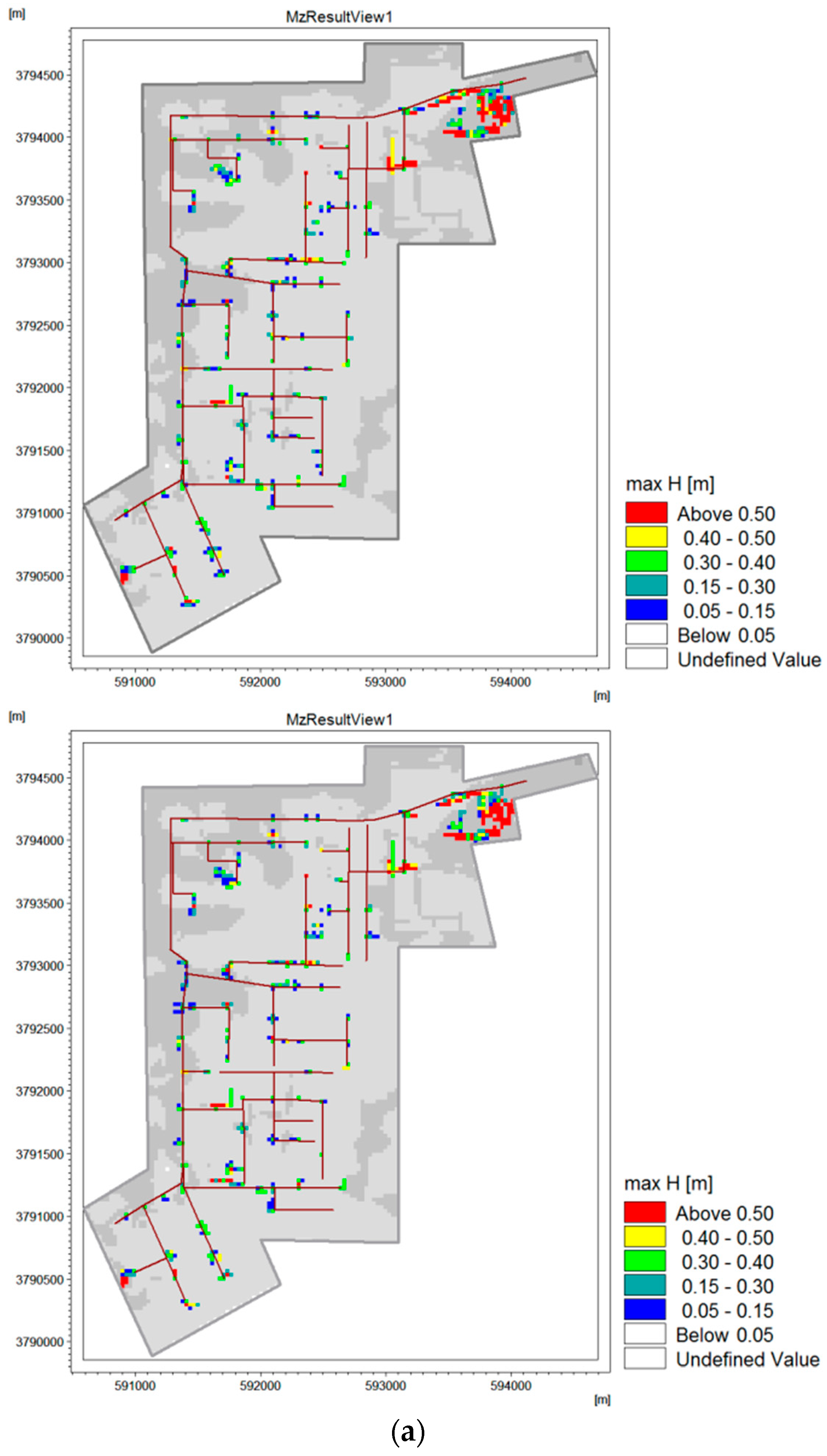
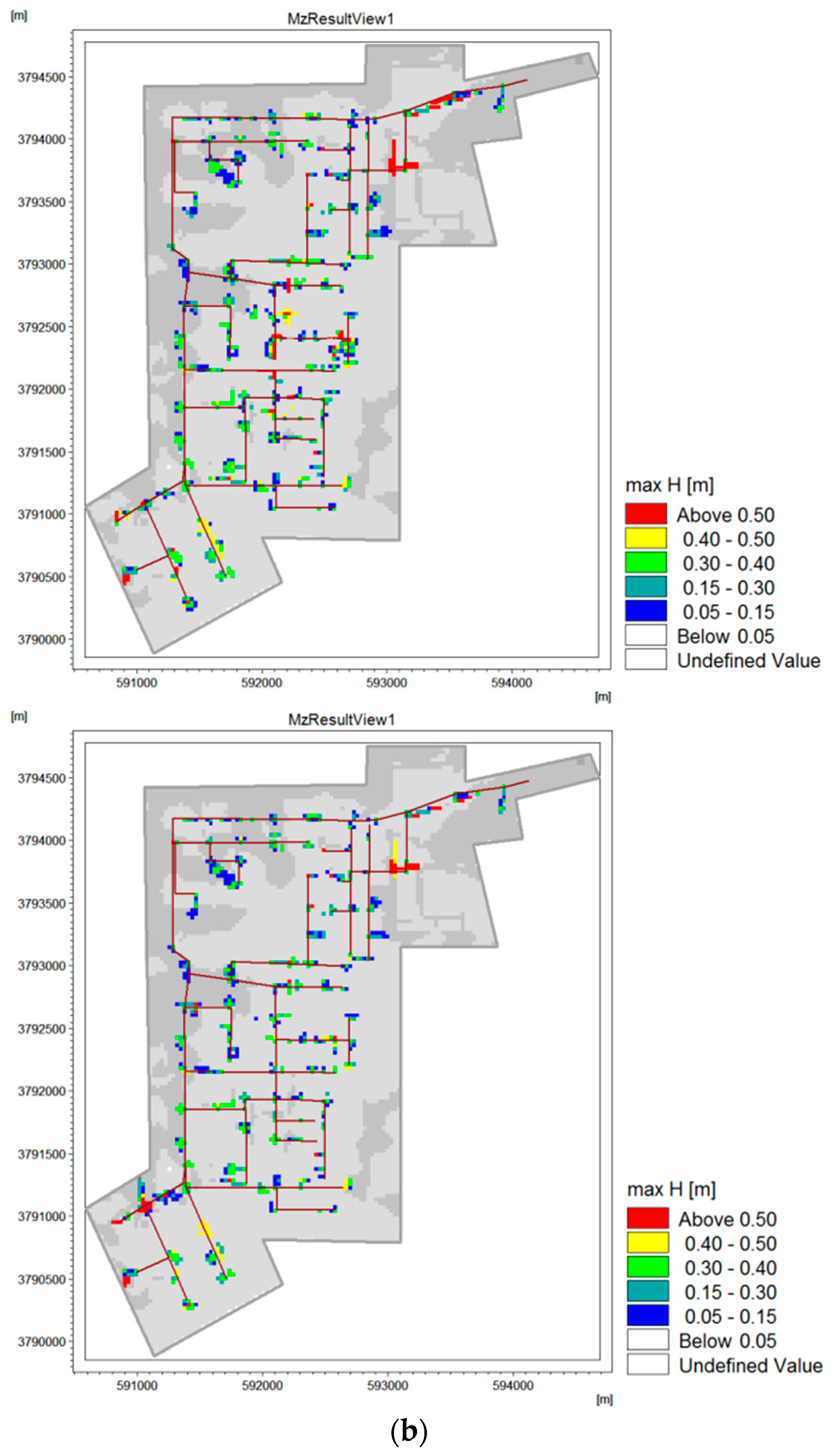
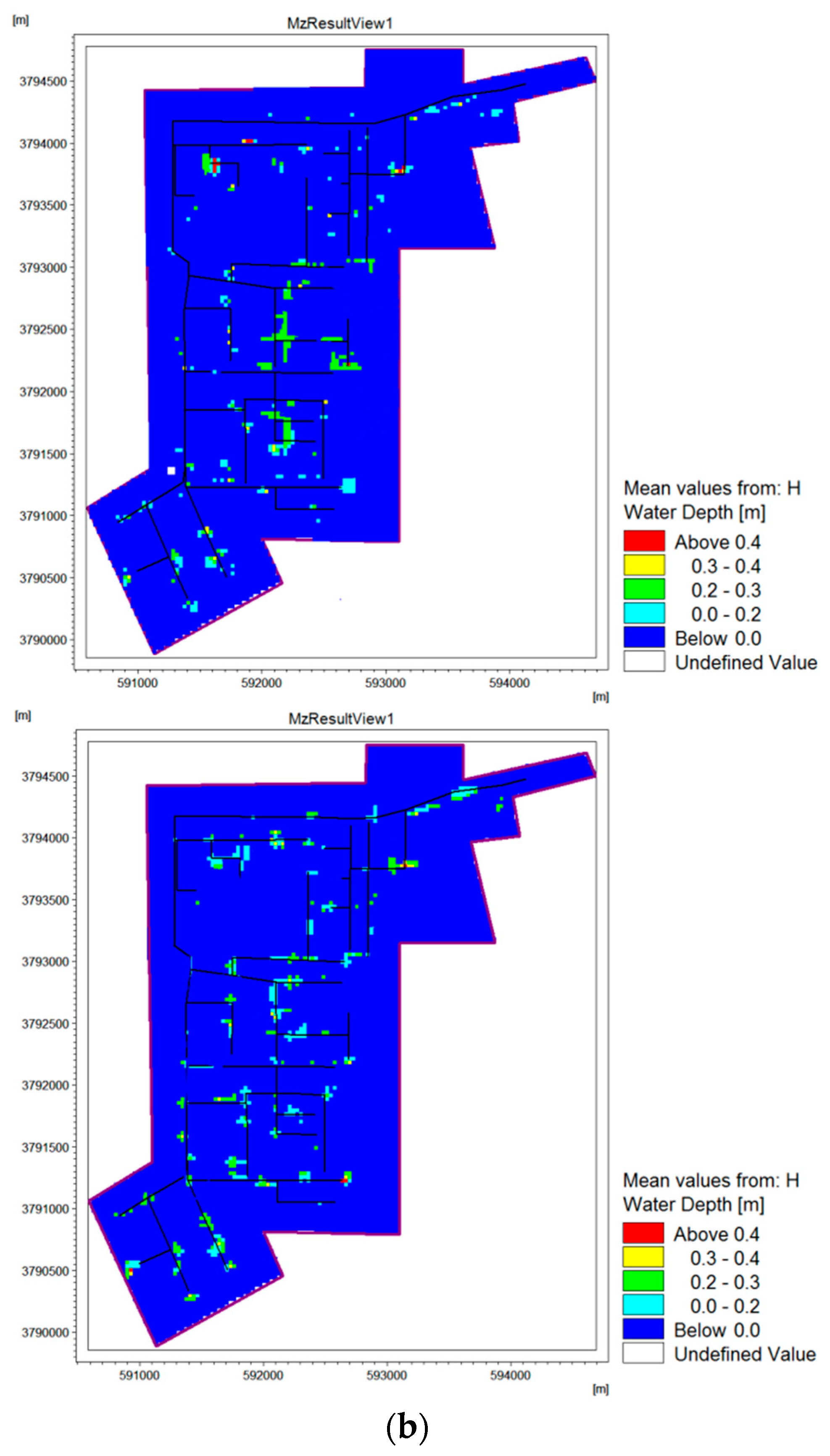
The model used the above six kinds of design rainfalls to simulate the drainage system capacity of the study area to assess the distribution of waterlogging areas in the study area with and without rain garden regulation. In Figure 5, (a) is the maximum submerged depth distribution map with no rain garden regulation and rain garden regulation under the five-year design rainfall condition, and (b) is under the twenty-year design rainfall condition.

Comparing the distribution maps of the submerged range at different water depths under different rainfall recurrence intervals, it is not difficult to see that there is a positive correlation between water accumulation range, water accumulation depth, and design rainfall recurrence interval. Moreover, rain garden has a certain degree of regulation effect on the study area. In the Outdoor Drainage Design Code [19], it is generally considered that storm water accumulation below 15 cm does not constitute an impact on traffic or other hazards [20]. In order to further quantify the relationship between submerged area and submerged depth in different design rainfall recurrence intervals under rain garden and no rain garden regulation,

Table 5. Submerged range at different water depths.

Submerged Area (ha)		Submerged Water Depth
		0.05–0.15 m	0.15–0.3 m	0.3–0.4 m	0.4–0.5 m	>0.5 m	Total	15 cm or More Product Percentage of Water Area
1a	NRG	4.32	2.88	2.70	1.17	0.99	12.06	64.18%
	RG	0.00	0.00	0.00	0.00	0.00	0.00	0.00%
2a	NRG	7.74	5.22	4.77	1.53	5.13	24.39	68.27%
	RG	5.76	4.50	2.97	0.99	2.52	16.74	65.59%
5a	NRG	13.05	9.72	7.11	3.24	8.55	41.67	68.68%
	RG	12.60	9.63	6.66	2.70	8.01	39.60	68.18%
10a	NRG	21.15	19.89	13.05	3.87	10.26	68.22	69.00%
	RG	16.38	15.12	9.63	2.43	8.73	52.29	68.67%
20a	NRG	27.00	25.74	14.04	5.58	16.20	88.56	69.51%
	RG	20.70	19.26	10.17	3.87	13.23	67.23	69.21%
50a	NRG	28.89	28.26	16.38	7.11	17.82	98.46	70.66%
	RG	26.46	25.11	15.12	6.57	16.02	90.36	70.36%

shows specific submerged areas with different depths of water classification.

It can be seen from Table 5 that as the submerged depth increases, the submerged area under the depth decreases gradually, and the percentage of the total area of accumulated water above 15 cm gradually increases with the increase of the recurrence interval. In the six rain events with different recurrence intervals, the results of the submergence of each flood within the rain gardens reached a better reduction rate. The reduction effect of rain garden regulation decreases with the increase of rainfall intensity. In the course of short-term rainfall, the reduction rates of flooding inundation areas were 0.50%, 2.68, and 64.18%, respectively, and the reduction rates of flooded inundation areas in the long-term rainfall were 0.30%, 0.30%, and 0.32%, respectively.

3.2.2. Submerged Range at Different Submerged Periods

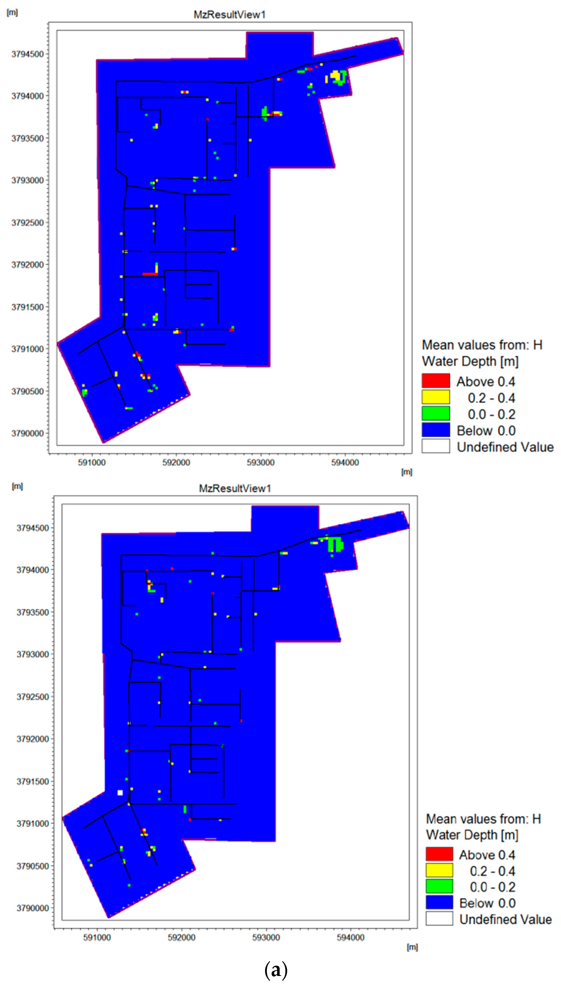
In addition to the depth of submergence, the duration of submergence is also an important assessment indicator of waterlogging hazards. Through statistics on the results of different rainfall recurrence intervals, the average depth of water is allocated according to the rainfall duration, and the distribution maps of the submerged area with rainfall duration are plotted for different recurrence intervals in the study area. In Figure 6, (a) is the submerged area distribution map over the duration of rainfall with no rain garden regulation and rain garden regulation under the five-year design rainfall condition, and (b) is under the twenty-year design rainfall condition.

From the figures, it can be seen that the areas with long periods of accumulated water are mainly concentrated in the places where the depth of accumulated water is relatively large. This is because the deeper water is generally located at a lower elevation, and it is difficult to exclude the accumulation of water. Comparing the statistics of the submerged area with different durations of submergence depth greater than 15 cm (traffic influence time) under different frequency rainstorm with the rain garden and no rain garden regulation, the results are shown in

Table 6. Submerged range at different submerged periods.

Rainfall Lasted	Submerged Area (ha)		Submerged Period
			30–60 min	60–90 min	90–120 min	120–150 min	>150 min	Total
3 h	1a	NRG	3.06	1.17	0.63	0	0	4.86
		RG	0	0	0	0	0	0
	2a	NRG	5.49	3.87	1.98	0	0	11.34
		RG	3.96	1.53	1.26	0	0	6.75
	5a	NRG	10.89	8.82	2.7	0	0	22.41
		RG	9.99	6.66	1.89	0	0	18.54
	Submerged Area (ha)		Submerged Period
			0.5–1 h	1–5 h	5–10 h	10–15 h	>15 h	Total
24 h	10a	NRG	16.02	11.43	9.27	5.67	0	42.39
		RG	13.68	10.17	8.46	3.96	0	36.27
	20a	NRG	17.91	13.32	11.34	6.39	0	48.96
		RG	15.12	12.33	10.53	5.76	0	43.74
	50a	NRG	22.05	14.67	13.14	7.02	0	56.88
		RG	19.62	14.22	12.51	6.48	0	52.83

.

As can be seen in Table 6, the submerged time is delayed with an increase in the recurrence interval. The duration of long-term rainfall flooding was significantly longer than that of the short-term, and the waterlogging phenomenon regulated by the rain garden was significantly less effective than that of no rain garden regulation. In the short-term rainfall condition, the submerged area reduction rates of submerged 120 min or less are 17.27%, 40.48%, and 100%, respectively; in the long-term rainfall, the submerged area submerged reduction rates of less than 15 h are 7.12%, 10.66%, and 14.44%, respectively. This is because as the recurrence interval increases, the generated runoff increases and the flow into the drainage pipe also increases. However, the capacity of the drainage pipeline is limited by the size of the pipeline, and there is a phenomenon that the time for retreating water increases as the recurrence interval increases.

3.2.3. Assessment of Waterlogging Risk in the Study Area

Using the MIKE model, a waterlogging risk analysis model suitable for the study area was established. The hazards of urban surface water accumulation should comprehensively consider the depth of water depth and the duration of accumulated water in two aspects to carry out risk analysis, and further evaluate the impact of urban storm on urban areas.

According to the relevant standards for prevention of waterlogging in the Outdoor Drainage Design Code, the depth of accumulated water in the road must not exceed 15 cm. At the same time, with reference to the Xi’an waterlogging study [4], considering the depth and duration of the accumulated water, the risk level of the model simulation results is divided, and the corresponding submerged areas of different levels are calculated. This article divides the risk into three levels: a slight accumulation, a medium accumulation, and a severe accumulation.

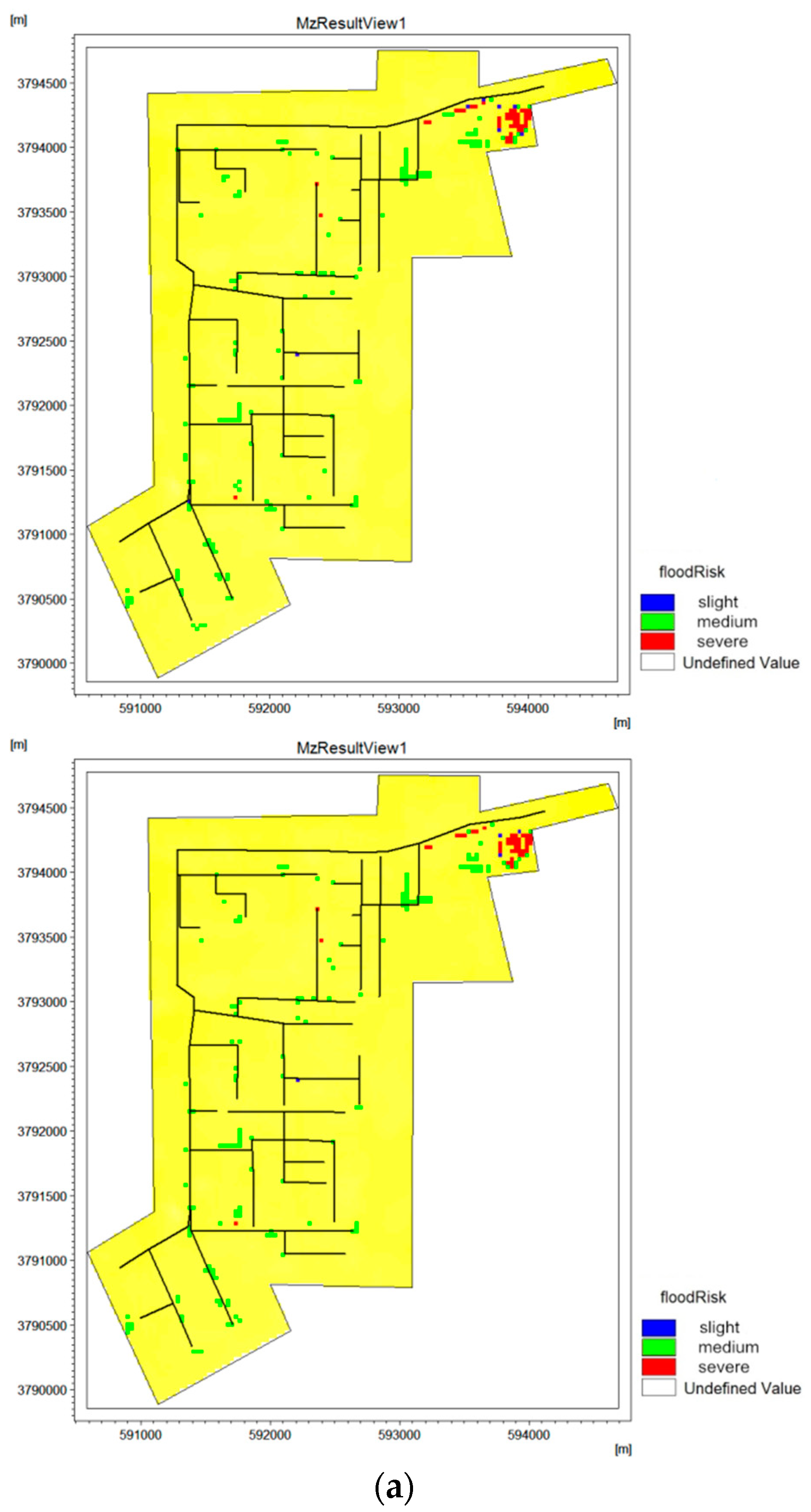
Based on the above criteria for classification of waterlogging risk, according to the distribution map of waterlogging in the study area, the automatic modeling and intelligent analysis system (AMIAS) was used to determine the accumulated water area and waterlogging risk level map. Different colors represent the water areas with different risk levels. In Figure 7, (a) is the distribution of waterlogging risk in the study area with no rain garden regulation and rain garden regulation under the five-year design rainfall condition, and (b) is under the twenty-year design rainfall condition. The criteria for the classification of risk levels and the submerged area statistics for the corresponding levels are shown in

Table 7. Classification standard and area statistics of waterlogging.

Rainfall Lasted	Rainfall Recurrence Interval	Regulatory Methods	Waterlogging Risk Levels
			A Slight Accumulation a		A Medium Accumulation b		A Severe Accumulation c
			Submerged Area/ha	Road Submerged Area/ha	Submerged Area/ha	Road Submerged Area/ha	Submerged Area/ha	Road Submerged Area/ha
3 h	1a	NRG	0.00	0.00	3.15	1.71	6.30	0.00
		RG	0.00	0.00	0.00	0.00	0.00	0.00
	2a	NRG	0.09	0.00	6.48	2.79	2.79	0.72
		RG	0.00	0.00	5.40	2.25	1.17	0.54
	5a	NRG	0.72	0.36	14.39	4.68	4.14	0.90
		RG	0.36	0.09	14.03	4.50	4.05	0.90
24 h	10a	NRG	0.09	0.00	22.40	8.10	4.05	1.98
		RG	0.00	0.00	16.55	6.66	1.26	0.27
	20a	NRG	0.18	0.00	30.41	10.71	7.20	2.43
		RG	0.36	0.00	20.60	7.92	2.88	1.35
	50a	NRG	0.45	0.00	36.79	13.40	7.29	2.16
		RG	0.24	0.00	36.69	10.08	7.25	1.70

Note: ^a Max H 15–60 cm and Duration 15–30 min; ^b Max H 15–60 cm and Duration 30–60 min; ^c Max H >60 cm and Duration >60 min.

.

From Figure 7, we can see that high-risk areas are mainly located in the northeast of the study area. From the topography, these areas have low topography, which is likely to cause water accumulation and result in high risk. In addition, it can be seen that when there was no rain garden regulation during the five-year rainfall recurrence interval, the accumulation in the area was dominated by medium accumulation, and the submerged area reached 25.19 ha. When there was rain garden regulation, the submerged area was reduced to 23.93 ha. In the event of a 20-year rainfall recurrence interval; when there was no rain garden regulation, the accumulation of the area was mainly medium and severe. The submerged area reached 50.93 ha, which seriously affected production and daily life. When there was rain garden regulation, the submerged area was reduced to 33.11 ha.

At the same time, by analyzing Table 7, we can see that the risk of accumulated water of the entire study area is mainly from the road. The road submerged area corresponding to different recurrence intervals accounted for more than 30% of the total submerged area. After adding the rain gardens, for the short-term rainfall, the percentage of the submerged area of the waterlogging risk area decreased by 100%, 29.81%, and 4.21%. For the long-term rainfall, the submerged area of the waterlogging risk area decreased by 32.88%, 36.90%, and 0.78%, respectively.

4. Conclusions

In the study area, 46 rain gardens were laid out, and the total area was 2% of the total area of the study area. Comparisons were made before and after laying rain gardens. The results showed that after the control measures of rain garden, for the flow peaks at the outlet of the study area, the reduction rate increased by 0.42% to 17.37%, the peak time of the flow rate was postponed by 1 to 6 min, the total runoff reduction rate increased by 1.93% to 9.69%, the overflow reduction rate was 6.74% to 65.23%, the overflow points reduction rate was 1.79% to 65.63%, and the overload pipelines reduction rate was 0% to 11.15% at different frequency rainfall events. Under different rainfall conditions, the peak concentration of SS decreased by 0.42% to 1.08% and the load reduction rate was 2.36% to 30.35% after rain garden measures were added. The peak COD reduction rate was 0.25% to 0.94%, and the load reduction rate was 2.37% to 30.11%. The TN peak concentration reduction rate was 0.15% to 0.65% and the load reduction rate was 2.34% to 30.08%. The TP peak concentration reduction rate was 0% to 1.07%, and the load reduction rate was 2.32% to 31.35%. The order of load reduction for each indicator is: TP > SS > COD > TN. Rain garden has a certain degree of control over the waterlogging, that is, the submersion ranges of different submerged depths and submerged durations are reduced by 0.30–64.18% and 7.12–100%, respectively. The AMIAS was used to carry out waterlogging risk assessment of the study area, and the statistics showed that the rain garden regulation range of the waterlogging risk area in the study area was 0.78% to 100%. The rain garden has a good control effect on urban storm runoff in terms of water volume and water quality, but as the recurrence interval increases, the control effect will decrease. The reason for this is that the construction of buildings has changed the direction of movement of the water flow, limiting it to accumulate along the road, and increasing the risk of water accumulation.

References

- Ana, E.V.; Bauwens, W. Modeling of the structural recreation of urban drainage pipes: The state of the art in statistical methods. Urban Water J. 2010, 7, 47–59. [Google Scholar] [CrossRef]
- Heaney, J.P. Optimization of integrated urban wet-weather control strategies. J. Water Res. Plan. Manag. 2005, 131, 307–315. [Google Scholar]
- Li, J.K.; Shen, B.; Dong, W.; Li, H.E.; Li, Y.J. Water contamination characteristics of a representative urban river in northwest china. Fresenius Environ. Bull. 2014, 23, 239–253. [Google Scholar]
- Li, J.K.; Li, Y.; Shen, B.; Li, Y.J. Simulation of rain garden effects in urbanized area based on SWMM. J. Hydroelectr. Eng. 2014, 33, 60–67. [Google Scholar]
- Dietz, M.E. Low impact development practices: A review of current research and recommendations for future directions. Water Air Soil Pollut. 2015, 22, 543–563. [Google Scholar] [CrossRef]
- Qin, H.P.; Li, Z.X.; Fu, G.T. The effects of low impact development on urban flooding under different rainfall characteristics. J. Environ. Manag. 2013, 129, 577–585. [Google Scholar] [CrossRef] [PubMed] [Green Version]
- Qi, H.J. Design and Performance Simulation of Low Impact Development Measures of Rainwater Management; Beijing University of Architecture: Beijing, China, 2013. [Google Scholar]
- Shao, Z.Y.; Zeng, Y.M.; Kang, W.; Hu, X.B.; Chai, H.X. Current features and future prospects of low impact development rainfall-runoff models for residential building areas. China Water Wastewater 2016, 32, 63–67. [Google Scholar]
- Chen, Y.; Samuelson, H.W.; Tong, Z. Integrated design workflow and a new tool for urban rainwater management. J. Environ. Manag. 2016, 180, 45–51. [Google Scholar] [CrossRef] [PubMed] [Green Version]
- Qin, H.P.; Soonthiam, K.; Yu, X.Y. Spatial variations of storm runoff pollution and their correlation with land-use in a rapidly urbanizing catchment in China. Sci. Total Environ. 2010, 408, 4613–4623. [Google Scholar] [CrossRef] [PubMed]
- Li, J.K.; Zhang, B.; Mu, C.; Chen, L. Simulation of the hydrological and environmental effects of a sponge city based on MIKE Flood. Environ. Earth Sci. 2018, 77. [Google Scholar] [CrossRef]
- Sharifan, R.A.; Roshan, A.; Aflatoni, M.; Jahedi, A.; Zolghadr, M. Uncertainty and sensitivity analysis of SWMM model in computation of manhole water depth and subcatchment peak flood. Procedia Soc. Behav. Sci. 2010, 2, 7739–7740. [Google Scholar] [CrossRef]
- Dreelin, E.A.; Fowler, L.; Ronald, C.C. A test of porous pavement effectiveness on clay soils during natural storm events. Water Res. 2006, 40, 799–805. [Google Scholar] [CrossRef] [PubMed]
- Zhang, J.Q.; Okada, N.; Tatano, H.; Hayakawa, S. Risk Assessment and Zoning of Flood Damage Caused by Heavy Rainfall in Yamaghchi Prefecture, Japan; Science Press: New York, NY, USA, 2002; pp. 162–170. [Google Scholar]
- Li, J.K.; Deng, C.N.; Li, H.E.; Ma, M.H.; Li, Y.J. Hydrological environmental responses of LID and approach for rainfall pattern selection in precipitation data-lacked region. Water Resour. Manag. 2018. [Google Scholar] [CrossRef]
- Sun, Y.W. Eco-Hydrological Impacts of Urbanization and Low Impact Development; Northwest A&F University: Xi’an, China, 2011. [Google Scholar]
- Zhou, X.F. The Study of Waterlogging Simulation and Risk Assessment Based on MIKE Flood Model in Yuncheng City; Xi’an University of Technology: Xi’an, China, 2017. [Google Scholar]
- Pan, G.Y.; Xia, J.; Zhang, X.; Wang, H.P.; Liu, E.M. Research on simulation test of hydrological effect of bio-retention units. Water Resour. Res. 2012, 305, 13–15. [Google Scholar]
- Zhang, C.; Zhi, X.H.; Zhu, G.H.; Chen, Y. The new version of “Outdoor Drainage Design Code” local revision interpretation. Water Wastewater Eng. 2012, 38, 34–38. [Google Scholar]
- Wang, D. Study on Urban Waterlogging Simulation in Qujiang New District of Xi’an Based on MIKE Model; Xi’an University of Technology: Xi’an, China, 2017. [Google Scholar]
Figure 1.
Models of 1D drainage (a) and 2D coupling (b).
Figure 2.
Parameter calibration of (a) water quantity and water quality including (b) suspended solids (SS), (c) chemical oxygen demand (COD), (d) total nitrogen (TN), and (e) total phosphorus (TP).
Figure 3.
Parameters validation of (a) water quantity, pollutant validation of (b) SS, (c) COD, (d) TN, and (e) TP.
Figure 4.
Simulation of rain garden in the MIKE model.
Figure 5.
Distribution of rainstorm waterlogging at different maximum submerged depth. (a) Distribution of rainstorm waterlogging at different maximum submerged depth during the 5- year recurrence interval with no rain garden and rain garden regulation; (b) Distribution of rainstorm waterlogging at different maximum submerged depth during the 20-year recurrence interval with no rain garden and rain garden regulation.
Figure 6.
Distribution of rainstorm waterlogging at different submerged periods. (a) Distribution of rainstorm waterlogging at different submerged periods during the 5-year recurrence interval with no rain garden and rain garden regulation; (b) Distribution of rainstorm waterlogging at different submerged periods during the 20-year recurrence interval with no rain garden and rain garden regulation.
Figure 7.
Distribution of the waterlogging risk. (a) Distribution of the waterlogging risk during the 5-year recurrence interval with no rain garden and rain garden regulation; (b) Distribution of the waterlogging risk during the 20-year recurrence interval with no rain garden and rain garden regulation.