Rainfall Generation Using Markov Chain Models; Case Study: Central Aegean Sea

Abstract

Generalized linear models (GLMs) are popular tools for simulating daily rainfall series. However, the application of GLMs in drought-prone areas is challenging, as there is inconsistency in rainfall data during long and irregular periods. The majority of studies include regions where rainfall is well distributed during the year indicating the capabilities of the GLM approach. In many cases, the summer period has been discarded from the analyses, as it affects predictive performance of the model. In this paper, a two-stage (occurrence and amounts) GLM is used to simulate daily rainfall in two Greek islands. Summer (June–August) smooth adjustments have been proposed to model the low probability of rainfall during summer, and consequently, to improve the simulations during autumn. Preliminary results suggest that the fitted models simulate adequate rainfall occurrence and amounts in Milos and Naxos islands, and can be used as input in future hydrological applications.

1. Introduction

The inadequate rain gauge network and the limited available rainfall records are critical factors that constrain rainfall modelling and the investigation of long-term rainfall variation. As a result, Generalized linear models (GLMs) have been proposed, as they are capable of generating and adequately representing the temporal non-stationarities of daily rainfall. Reference [1] made one of the preliminary studies as they fitted two state Markov chain models to simulate single-site daily rainfall occurrence and amounts in Morogoro, Tanzania. Chandler and Wheater [2,3] extended the work of Stern and Coe by using a two-stage GLM to predict the spatial probability distribution of daily rainfall in Western Ireland. They incorporated long-term climatic predictors to describe variations in historical rainfall records, and to investigate possible climate change. Their work has been a baseline for many studies published afterwards ([4,5,6] amongst others). Spatial models have also been fitted in many areas across the world in order to infill missing values in observed rainfall records. Reference [7] fitted GLMs in North-East Botswana to impute missing rainfall records for 24 years. They computed the Anscombe residuals from sites with observed rainfall in order to simulate adequate daily records with no missing values. The GLM framework has also been used to model the discrete and continuous nature of daily rainfall variables simultaneously [8,9,10] by fitting Tweedie GLMs to generate monthly rainfall data in 220 Australian stations. They incorporated 4 climatological variables, and the fitted models adequately predicted the preceding month. The importance of developing models for generation of rainfall series at ungauged sites has been widely reported, and diverse approaches have been proposed. For instance, in [11], a GIS-based model for the assessment of monthly time-series of several key hydro-climatic variables at the basin scale (rainfall amongst others) was developed in an area (Southern Italy) similar to climate characteristics of the selected study area [12]. However, the application of GLMs in areas, where extended dry periods or severe drought events are present, is challenging, as the probability of rainfall during a summer period is very low. The fitted models usually over-predict rainfall absence during summer, while the model performance is significantly affected during autumn.

In this study, daily rainfall series have been provided from the Hellenic National Meteorological Service (HNMS) for Milos and Naxos meteorological stations for the period 1955–2010. Descriptive analysis has been performed at the monthly, seasonal and annual time scales to understand the various aspects of rainfall behavior. The GLM framework has been used; occurrence and amounts models have been fitted to reproduce rainfall properties for each island. The long dry periods that exist in Milos and Naxos indicated the need to further exploit the investigation of alternatives. The incorporation of summer smooth adjustments was proposed (in the view of the extended monthly smooth adjustments as presented by [13]), in order to improve the total predictive performance of the fitted models. The specific characteristics of the investigated rainfall data (absence of rainfall for extensive periods) have not been thoroughly advanced in literature for rainfall simulation purposes. The presented methodological approach based on GLMs with summer smooth adjustments performed well in capturing the rainfall behavior and overcoming the limitations of the standard GLM approach in under-predicting rainfall occurrence during autumn. Various model checks have been performed to investigate the model performance and the systematic structure that is explained by the fitted models at different time scales.

Exploratory Analysis

Milos and Naxos are located in the central Aegean Sea. The climate in both islands is of Mediterranean type with long dry summers and mild winters. Although the Aegean Islands extend over a relatively small geographical area, they show variability in meteorological variables due to the geomorphology and the air–sea interaction. Figure 1 presents the available data, and the locations of the stations are shown in

Table 1. Descriptive analysis of rainfall series.

Station	Rainfall Record	Longitude	Latitude	Altitude	Missing Records
Milos	1955–2010	36.43	24.27	183	49
Naxos	1955–2010	36.60	25.23	9	10
Rainfall Indices
Station	Statistic	Annual Rainfall	Number of dry days	Number of dry days during summer	Maximum number of consecutive dry days
Milos	Mean	406.54	305.73	91.12	119.38
	SD	106.09	11.28	1.06	32.65
Naxos	Mean	365.65	304.59	90.91	113.75
	SD	107.66	12.56	1.27	34.58

, along with a set of meteorological indices. In cooperation with the HNMS, data quality control has been made, and all missing or dubious daily rainfall records have been discarded from the data set according to the HNMS protocol.

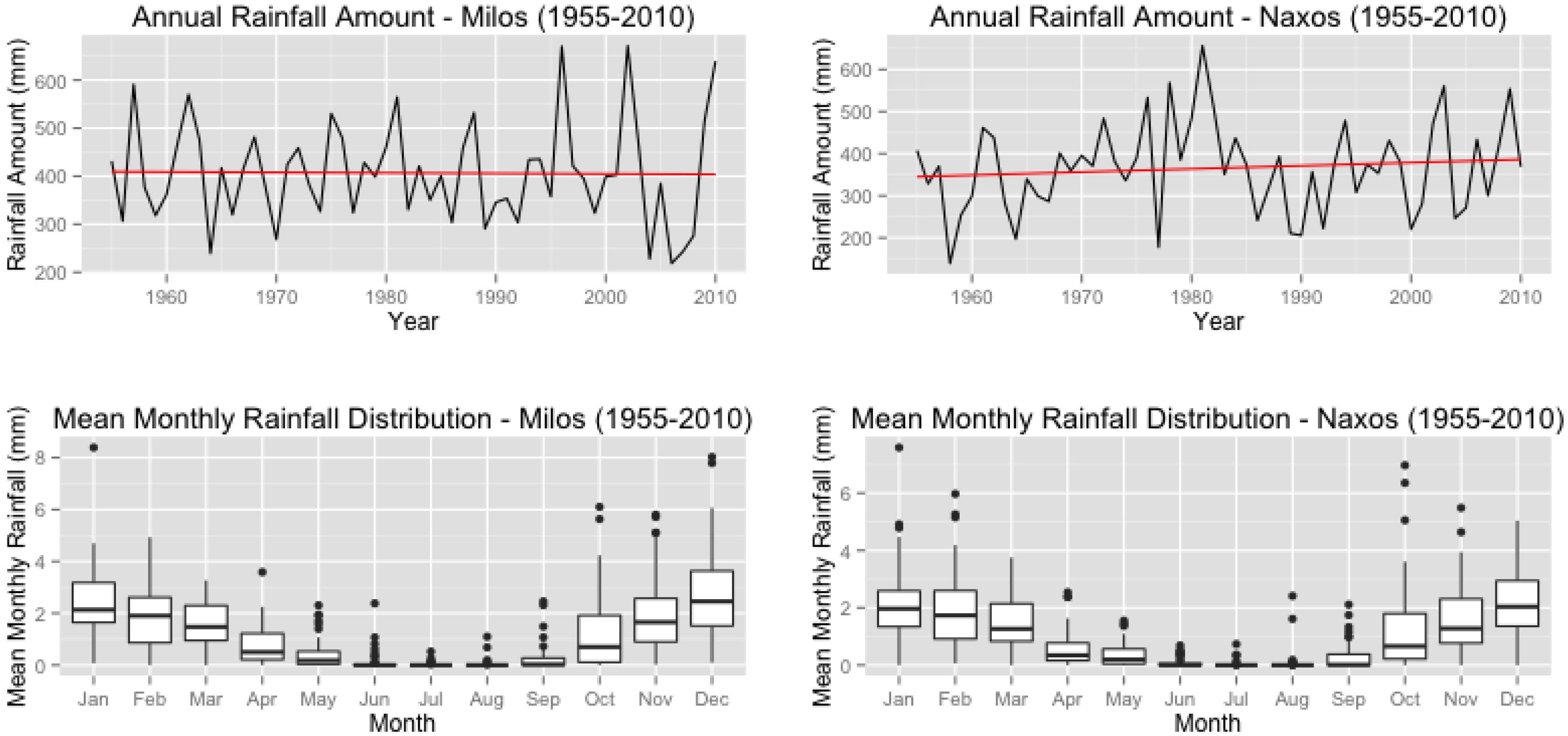
Exploratory data analysis has been performed in both the Milos and Naxos stations in order to examine the characteristics that led to possible variations during the reference period. A set of precipitation indices were investigated, namely, the annual rainfall, the annual proportion of rainy days and the mean daily winter rainfall. In the Milos station, the annual rainfall amounts were too variable (e.g., 100 mm in 1956 and 550 mm in 1985) and this high variability tended to be more intense in the beginning of 1990 until 2010 with extreme dry and wet years. However, there is not clear evidence for a changing rainfall pattern. As expected in the Eastern Mediterranean region, rainfall amounts during rainy periods affected the annual rainfall amounts and suggested that it would be useful to examine rainfall during winter.

As presented in Figure 1, it is clear that the mean monthly rainfall during the summer period was almost zero, while in winter period, the activity was much higher. However, rainfall analysis during the winter period did not present any significant trends. Exploratory analysis for the Naxos site suggested that the annual rainfall presented a long-term cyclical trend that was reflected by the annual proportion of rainy days for the entire period. The Mann–Kendall test for trends has been used to identify possible significant trends in the annual rainfall amount series for both Milos and Naxos meteorological records. There is some indication that annual rainfall series tended to increase since 1990s (1990–2010); however, the trend of the annual rainfall remained relatively stable during the reference period (1955–2010), which is similar to the trend identified in Milos. Similar results were observed in the mean winter rainfall with the series remaining stable.

The findings of the exploratory data analysis followed the results of many studies based on trend detection of precipitation series in the eastern part of Mediterranean ([14,15] amongst others).

2. Materials and Methods

The GLM framework has been used to predict the probability distribution of daily rainfall conditional on the features’ vector. In this study, a two-stage approach has been adopted. Firstly, an occurrence model has been fitted to predict the probability distribution of rainy and dry days at a site using logistic regression:

$$\ln \left(\frac{{\mathrm{p}}_{\mathrm{i}}}{1-{\mathrm{p}}_{\mathrm{i}}}\right)={{\mathrm{x}}^{\prime }}_{\mathrm{i}}\beta$$

(1)

where ${\mathrm{p}}_{\mathrm{i}}$ is the probability of rain for the ${\mathrm{i}}^{\mathrm{th}}$ day, conditional on a p-dimensional feature vector represented by $x_i={(x_{0i},x_{1i},\dots ,x_{pi})}^{\prime }$, ${\mathrm{x}}_{0\mathrm{i}}=1$, and $\beta ={({\beta }_0,{\beta }_1,\dots ,{\beta }_p)}^{\prime }$ is the p-dimensional vector of coefficients. A rainy day is defined when the rain gauge measurement is ≥0.1 mm, and a dry day is defined when the rain gauge measurement is <0.1 mm.

At the second stage of the study, the amounts model describes the probability distribution function of daily rainfall amounts on rainy days using a Gamma regression model. Let $Y_i$ be the amount of rainfall for the ${\mathrm{i}}^{\mathrm{th}}$ rainy day. The distribution of $Y_i$ is assumed to be Gamma with a shape parameter ν considered to be stable throughout the observational period and a scale parameter ${I?}_i$. Note that the Gamma distribution is considered to be appropriate for nonnegative right skewed data, namely, characteristics typically exhibited by meteorological data. For the mean, which is given by $\mathrm{I}{\_}_{\mathrm{i}}=\frac{I\_}{I{?}_i}$, conditional on the features’ vector ${\mathrm{x}}_{\mathrm{i}}$, we considered the logarithmic transformation as following [16]:

$$\ln ({\mathsf{\mu }}_{\mathrm{i}})={{\mathrm{x}}^{\prime }}_{\mathrm{i}}\beta$$

(2)

Daily rainfall series are time dependent observations, and as a result, previous days’ rainfall has been incorporated into the feature vector. For this reason, the Generalised Autoregressive Models theory has been applied using the standard iterative weighted least squares algorithm and consequently maximizing the partial likelihood function, instead of the likelihood function [17].

2.1. Selection of Appropriate Predictors

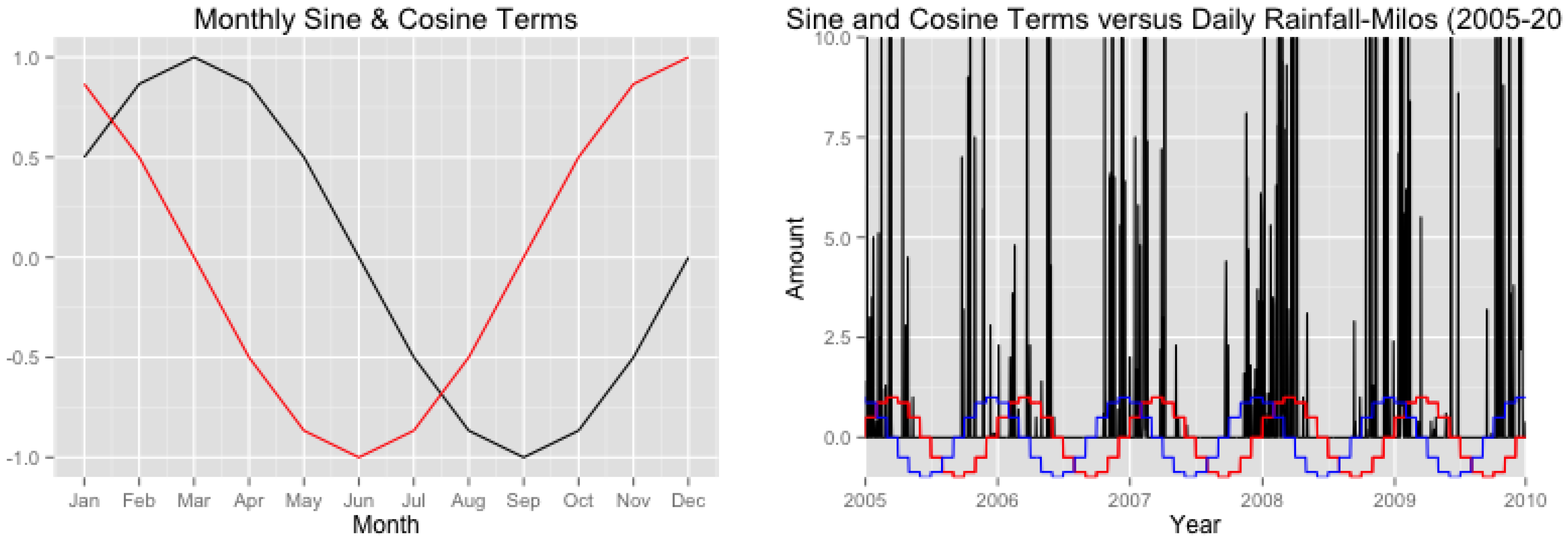
Due to the high dimensionality of the data set (approximately 20.400 observations per station) the selection of an appropriate set of predictors was not clear from the beginning of the study. For this reason, various plots and regression models were evaluated in aggregated data in order to investigate which predictors might prove useful. Lag 1 and Lag 2 autocorrelation terms were selected to model the rainfall persistence. The seasonal dependence (winter and summer periods) was captured using annual sine and cosine functions that vary smoothly during the year, which were described as $sin(2\times \pi \times \frac{month}{12})$ and $cos(2\times \pi \times \frac{month}{12})$, respectively.

As presented in Figure 2, the monthly sine term reached its maximum in March and its minimum in September (spring and autumn seasons), while the monthly cosine effect reached its maximum in December and its minimum in June (winter and summer seasons). The monthly sine and cosine terms seemed to be in agreement with the annual rainfall cycle, as presented in Figure 2. The annual trend function has been included in the fitted models in order to capture the variability that might be attributed to climate change variations.

Adjustments for individual month were added using shifted bisquare functions, as presented by [13]. However, the greatest challenge of this study was to deal with the over-prediction of daily rainfall absence during summer, which resulted in a systematic under-prediction of the daily rainfall occurrence during autumn. Therefore, a 3-month (June–August) adjustment was proposed:

$$(d)={\left[1-{\left(\frac{2d-(l+1)}{(l+1)}\right)}^2\right]}^2(d=1,\dots , l)$$

(3)

where $d$ is the day of the 3-month period and $l$ is the total number of the summer days. This function takes its maximum value during July, when the over-prediction of rainfall occurrence is more intense, and decays to zero at the beginning and the end of the summer. After the model fitting process, a number of diagnostic tests have been applied to assess each model separately.

2.2. Model Performance

There are a number of statistical model diagnostics in literature that can be used to assess the model predictive performance [18,19]. The Pearson residuals for an observation $Y_i$ are presented in the following form:

$$r_i=\frac{Y_i-{\mu }_i}{{\sigma }_i}$$

(4)

where ${\mu }_i, {\sigma }_i$ are the mean and standard deviation, respectively. If the fitted model is correct, the Pearson residuals should have mean 0 and variance 1. The Pearson residuals were used to check if the systematic structure has been captured adequately by the fitted model. For this reason, various plots have been incorporated in this study to assess whether the residuals lie within the additional 95% confidence bands at different time scales. When the probability distribution function of the variable of interest $Y_i$ is not normal, the Pearson residuals fail to have the properties of normal-theory residuals [18]. In this case, the Anscombe residuals were used for the amounts model and taken in the form as following:

$${\alpha }_{\iota }={\left(\frac{Y_i}{{\mu }_i}\right)}^{1/3}$$

(5)

If the gamma assumption, which is conditional on the features’ vector, is correct, all residuals should have Gaussian distributions.

3. Modeling Results

3.1. Occurrence Models

Table 2. Occurrence models.

Milos
Model	Description	Parameters	Log-Likelihood	AIC
1.O.M	$y_{t\mathbf{-}\mathbf{1}}\mathbf{+}{y}_{t\mathbf{-}\mathbf{2}}\mathbf{+}\mathrm{Sine} \mathrm{Term}\mathbf{,}\mathbf{+}\mathrm{Cosine} \mathrm{Term}$	4	−7098.75	14,207.50
2.O.M	$1.\mathrm{O}.\mathrm{M}+y_{t\mathbf{-}\mathbf{1}}\mathbf{\ast }{y}_{t\mathbf{-}\mathbf{2}}\mathbf{+}\mathrm{Sine} \mathrm{Term}\mathbf{\ast }\mathrm{Cosine} \mathrm{Term}\mathbf{+}{y}_{t\mathbf{-}\mathbf{1}}\mathbf{\ast }\mathrm{Sine} \mathrm{Term}\mathbf{+}{y}_{t\mathbf{-}\mathbf{1}}\mathbf{\ast }\mathrm{Cosine} \mathrm{Term}$	8	−6996.22	14,010.44
3.O.M	$2.\mathrm{O}.\mathrm{M}+\mathrm{Trend}$	9	−6990.49	14,000.97
4.O.M	$3.\mathrm{O}.\mathrm{M}+{\mathrm{Bisquare}}_{\mathrm{Summer}}\mathbf{+} {\mathrm{Bisquare}}_{\mathrm{Summer}}\mathbf{\ast }\mathrm{Sine} \mathrm{Term}\mathbf{+} {\mathrm{Bisquare}}_{\mathrm{Summer}}\mathbf{\ast }\mathrm{Cosine} \mathrm{Term}$	12	−6972.13	13,970.25
Naxos
Model	Description	Parameters	Log-Likelihood	AIC
1.O.N	$y_{t\mathbf{-}\mathbf{1}}\mathbf{+}{y}_{t\mathbf{-}\mathbf{2}}\mathbf{+}\mathrm{Sine} \mathrm{Term}\mathbf{,} \mathbf{+} \mathrm{Cosine} \mathrm{Term}$	4	−7152.42	14,314.83
2.O.N	$1.\mathrm{O}.\mathrm{M}+y_{t\mathbf{-}\mathbf{1}}\mathbf{\ast }{y}_{t\mathbf{-}\mathbf{2}}\mathbf{+} \mathrm{Sine} \mathrm{Term}\mathbf{\ast }\mathrm{Cosine} \mathrm{Term}\mathbf{+} y_{t\mathbf{-}\mathbf{1}}\mathbf{\ast }\mathrm{Sine} \mathrm{Term}$	7	−7054.65	14,125.29
3.O.N	$2.\mathrm{O}.\mathrm{M}+{\mathrm{Bisquare}}_{\mathrm{Summer}}\mathbf{+}{\mathrm{Bisquare}}_{\mathrm{Summer}}\mathbf{\ast }{y}_{t\mathbf{-}\mathbf{1}}$	9	−7030.85	14,081.70

presents the occurrence models fitted in Milos (O.M) and Naxos (O.N) sites. Initially, simple models without interactions have been fitted and the use of additional predictors has improved the modeling results. The selection of the fitted models has been performed using the deviance criterion through the stepwise algorithm, while model checks on the model residuals indicated that the distributional assumptions were not violated.

As presented in

Table 3. Occurrence of Models 4.O.M (Milos) and 3.O.N (Naxos).

	Milos				Naxos
	Predictors	Description	Estimation	Std. Error	Predictors	Description	Estimation
	Constant		−2.34	0.06	Constant		−2.44
1		Previous day’s rainfall occurrence	1.91	0.08		Previous day’s rainfall occurrence	1.92
2		2 days before rainfall occurrence	0.49	0.07		2 days before rainfall occurrence	0.47
3	Monthly Effect	Monthly sine-effect annual cycle	0.81	0.05	Monthly Effect	Monthly sine-effect annual cycle	0.82
4	Monthly Effect	Monthly cosine-effect annual cycle	1.17	0.06	Monthly Effect	Monthly cosine-effect annual cycle	−1.06
5	Trend	Linear Trend	−0.004	0.00	Summer Effect	Smooth summer adjustment	−2.07
6	Summer Effect	Smooth summer adjustment	−17.92	6.91	Interactions	Interaction 1 and 2	−0.76
7	Interactions	Interaction 1 and 2	−0.61	0.1		Interaction 1 and 3	−0.22
8		Interaction 1 and 3	−0.38	0.08		Interaction 3 and 4	−0.48
9		Interaction 1 and 4	−0.28	0.09		Interaction 1 and 5	3.37
10		Interaction 3 and 4	−0.44	0.09
11		Interaction 3 and 6	−5.18	2.62
12		Interaction 4 and 6	−16.26	6.72
	Threshold		0.1 mm

, Models 4.O.M and 3.O.N (Table 3) were selected to model rainfall occurrence in Milos and Naxos sites, respectively. The introduction of the sine and cosine terms has captured the seasonal cycle of daily rainfall, while the site-specific seasonal patterns were captured by the summer smooth adjustments. The use of the indicator functions of the two previous days’ rainfall occurrence has captured the temporal dependence that is present in the data set, and the linear trend function was introduced to identify possible increasing or decreasing patterns of rainfall occurrence. Two-way interactions were incorporated into both models with the lag 1 and lag 2 autoregressive indicators and the seasonal smooth adjustments to identify possible interactions between the presence of rainfall during the last two days and the underlying seasonal patterns.

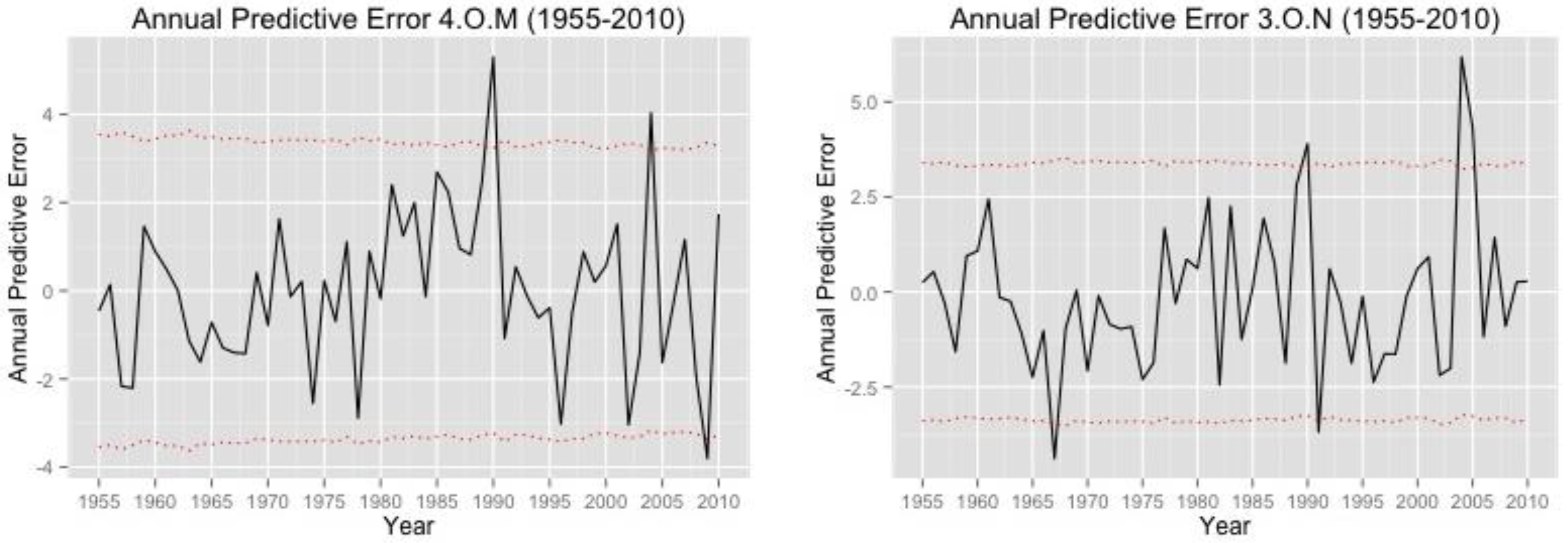
The annual performance of Models 4.O.M and 3.O.N was captured adequately (Figure 3), as the majority of the annual errors lied within the 95% confidence bounds. In Model 4.O.M, the highest discrepancy (under-prediction) was highlighted in 1990 and the observed annual rainfall record was 354 mm (the annual rainfall record during 1989 was 290.5 mm).

The overall assessment of Model 4.O.M indicated that the observed correct prediction was 84.60% and was in agreement with the expected correct prediction of 84.62%.

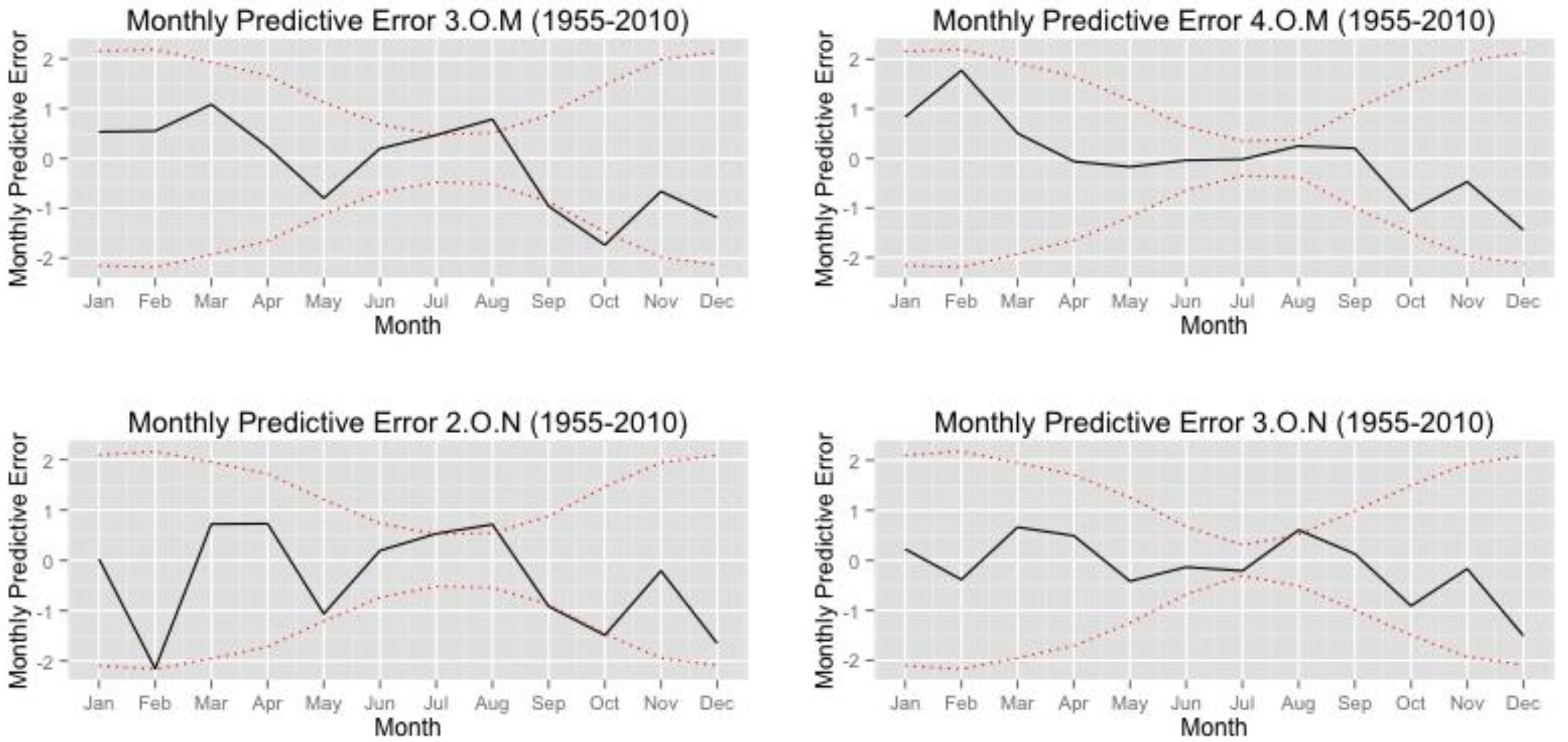
The monthly performance of the fitted models (Figure 4) indicated that both Models 3.O.M and 2.O.N over-predicted rainfall absence during the summer months, and consequently, under-predicted rainfall occurrence during October. The incorporation of the summer smooth adjustments (Equation (5)) has improved the model performance significantly. In Figure 4, it is clear that the difference between the observed and expected predictions lied within the 95% confidence bounds and led to more accurate models.

3.2. Amounts Models

Various amounts models have been fitted in Milos and Naxos stations (A.M: amounts model for Milos; A.N: amounts model for Naxos).

Table 4. Amounts models.

Milos
Model	Description	Number of parameters	Log-likelihood	AIC	Dispersion parameter
1.A.M	$y_{t\mathbf{-}\mathbf{1}}\mathbf{+}\mathrm{Sine} \mathrm{Term}\mathbf{,}\mathbf{+}\mathrm{Cosine} \mathrm{Term}$	3	−9573.8	19,156	2.71
2.A.M	1.A.M + ${\mathrm{Bisquare}}_{\mathrm{March}}\mathbf{+} {\mathrm{Bisquare}}_{\mathrm{September}}$	5	−95,650.0	19,142	2.71
3.A.M	2.A.M + Trend	7	−95,510.0	19,118	2.71
Naxos
Model	Description	Number of parameters	Log-likelihood	AIC	Dispersion parameter
1.A.N	$y_{t\mathbf{-}\mathbf{1}}\mathbf{+} \mathrm{Cosine} \mathrm{Term}$	2	−9289.7	18,585	2.81
2.A.N	1.A.N + ${\mathrm{Bisquare}}_{\mathrm{March}}\mathbf{+} {\mathrm{Bisquare}}_{\mathrm{August}}\mathbf{+}{\mathrm{Bisquare}}_{\mathrm{October}}$	5	−9236.3	18,485	2.65
3.A.N	2.A.N + Trend	7	−9219.2	18,454	2.67

presents the most adequate models of the analysis. Three models have been fitted to Milos to predict the probability distribution of the daily rainfall amount on a rainy day, conditional on the features’ vector.

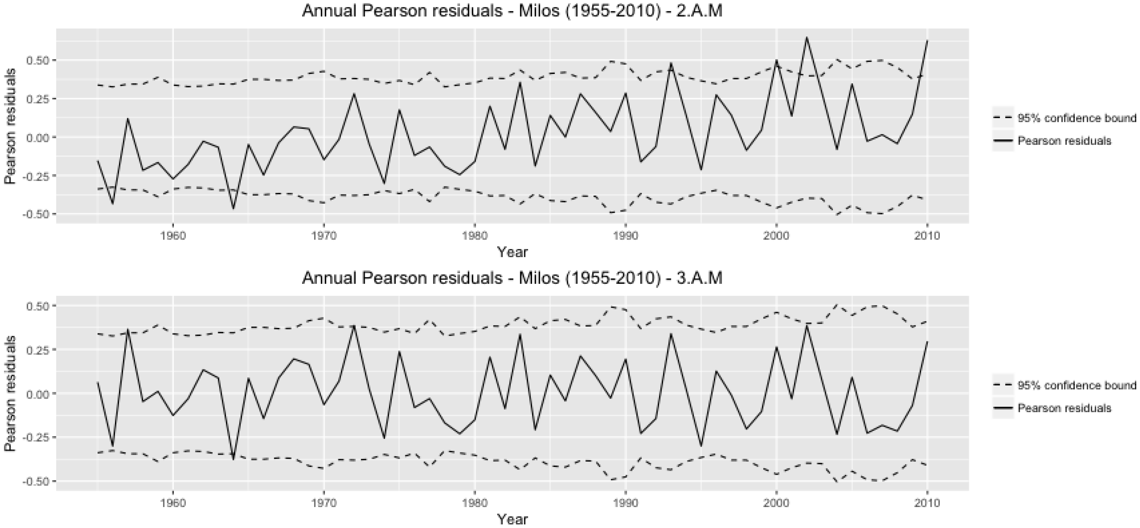
The analysis of the Pearson residuals at the monthly time scale for Model 1.A.M indicated that there were significant exceedances during March and October. For this reason, the monthly smooth adjustments have been incorporated into Model 2.A.M, in order to improve the monthly model performance. However, the Pearson residuals at the annual time scale for Models 1.A.M and 2.A.M (Figure 5) indicated the existence of a systematic upward trend that was present during the reference period, and after 2003, a number of discrepancies exceeded the 95% confidence bands.

In Milos, the introduction of the linear trend function and the additional interactions in Model 3.A.M are presented in in

Table 5. Amounts models.

Milos—3.Α.Μ				Naxos—3.Α.Ν
	Predictors	Description	Estimation	Predictors	Description	Estimation
	Constant		1.23	Constant		0.92
1		Previous days rainfall	0.25		Previous days rainfall	0.26
2	Monthly Effect	Monthly sine-effect annual cycle	−0.19	Monthly Effect	Monthly cosine-effect annual cycle	0.35
3	Monthly Effect	Monthly cosine-effect annual cycle	0.19	Monthly smooth adjustment	March effect	0.36
4	Monthly smooth adjustment	March effect	0.41	Monthly smooth adjustment	August effect	1.28
5	Monthly smooth adjustment	September effect	−0.67	Monthly smooth adjustment	October effect	0.50
6	Trend	Linear Trend	0.01	Trend	Linear Trend	0.01
7	Interaction	Interaction 1 and 6	−0.002	Interaction	Interaction 1 and 6	−0.003

. The annual structure of 3.A.M is shown in Figure 6, where the annual mean residuals lied within the 95% confidence bands. In Figure 6, Model 3.A.M presented a good agreement between the observed and simulated annual rainfall in Milos meteorological stations except for the year 2002 where the highest discrepancy (280.59 mm) was noticed.

One of the most important features of the fitting procedure is the physical interpretation of the interactions. Αn interaction between the linear trend function (Table 5) and the antecedent rainfall indicates the decayed significance of the antecedent rainfall in the predicted mean daily rainfall of the amounts model. In addition, the interaction between the long-term trend and the Fourier series provides essential information about drier summers and more rainy winters.

The value of the estimated trace values was 0.03 mm at both Milos and Naxos and corresponded to 3.15% and 2.75% of the entire data sets, respectively, indicating the importance of the incorporation of the trace into the modeling procedure. Additionally, the shape parameters that emerged both for Models 3.A.M and 3.A.N, were different for those indicating the exponential distribution, which is commonly used in many hydrological applications. The analysis of the Anscombe residuals indicated that the Gamma assumption conditional on the features’ vector holds both for Milos and Naxos amounts models.

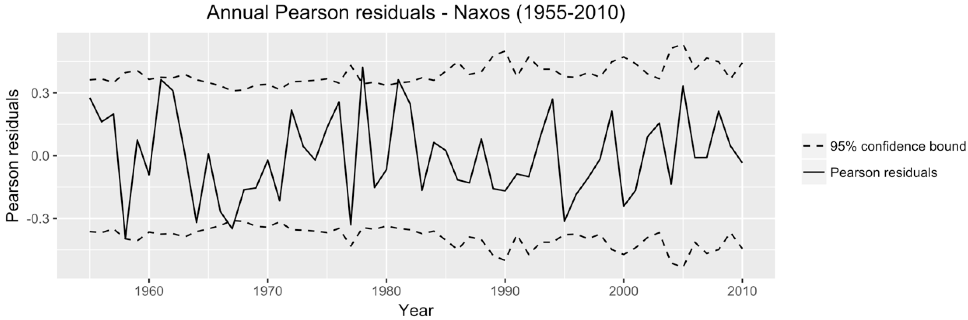
Three Models have also been fitted to the Naxos station in order to simulate daily rainfall on rainy days (Table 4). The monthly Pearson residuals indicated significant discrepancies between the observed and simulated rainfall during March, August and October. As a result, similar to the analysis performed for Milos, monthly smooth adjustments have been incorporated into Model 2.A.N to improve the model performance. However, the existence of a long-term upward trend in Model 2.A.N suggested the incorporation of a linear trend predictor. The performance of Model 3.A.N (Figure 7) suggested that the majority of the Pearson residuals lied within the 95% confidence bands, indicating that the annual structure has been captured adequately by the model.

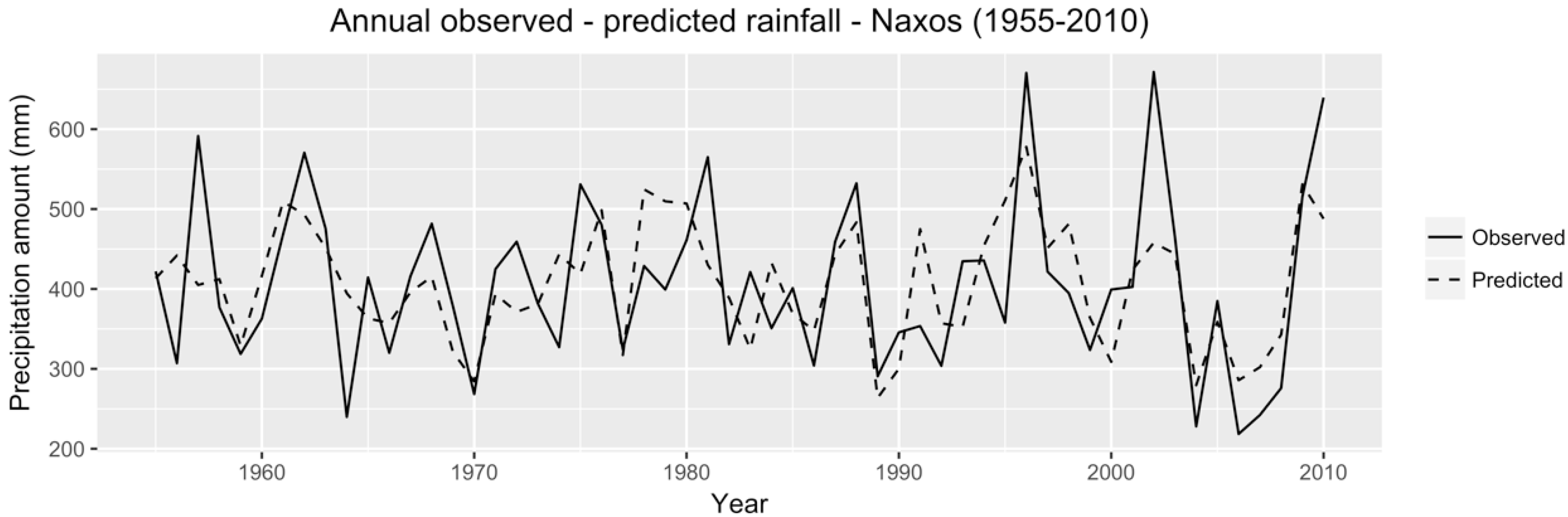
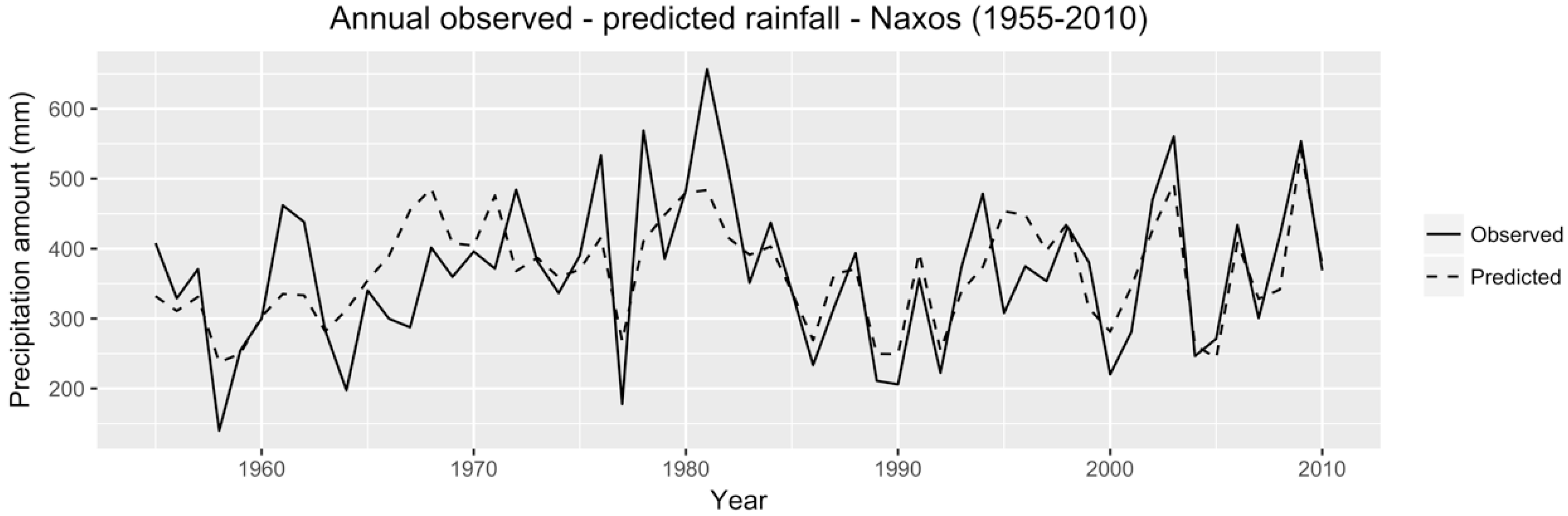
The performance of Model 3.A.N is presented in Figure 8 and presented a good agreement between the observed and simulated annual rainfall in Milos meteorological station except for the year 2002 where the highest discrepancy (280.59 mm) was noticed.

4. Conclusions

The application of autoregressive generalized linear models with summer smooth adjustments in areas, where severe drought is present, indicated that GLMs fitted adequately to the daily rainfall data with respect to the various model checks performed and presented in this paper. The stochastic nature of weather generators does not permit an interpretation of single events. Therefore, the model performance was evaluated for the entire time series. Issues regarding the magnitude of extreme precipitation events were observed. It is clear that the fitted models predicted dry days more accurately, but this can be accounted for the decreasing trend seen in the available data for the period 1955–2010, as well as the climate conditions in the eastern part of Mediterranean that display long dry periods. The application of the amounts model indicated that the simulated rainfall is close to the observed rainfall and can be further used in many studies related to the investigation of rainfall indices and trend detection in areas, where the problem of missing rainfall observations is important.

As presented, the proposed summer smooth adjustments have significantly improved the simulations during autumn in both data sets, overcoming the limitations of the standard GLM approach in under-predicting rainfall occurrence during autumn. The method was tested for two data sets from two Greek islands with noteworthy features; long dry periods during the summer pushed the simulation models to underperform during the subsequent period. The summer smooth adjustments captured those extreme patterns, allowing the amounts model in the GLM to preserve most standard statistics.

References

- Coe, R.; Stern, R.D. Fitting models to daily rainfall. J. Appl. Meteorol. 1982, 21, 1024–1031. [Google Scholar] [CrossRef]
- Chandler, R.E.; Wheater, H.S. Climate Change Detection Using Generalised Linear Models for Rainfall—A Case Study from the West of Ireland, I, Preliminary Analysis and Modelling of Rainfall Occurrence; Tech. Report; University College London: London, UK, 1998. [Google Scholar]
- Chandler, R.E.; Wheater, H.S. Climate Change Detection Using Generalised Linear Models for Rainfall—A Case Study from the West of Ireland, II, Modelling of Rainfall amounts on Wet Days; Tech. Report; University College London: London, UK, 1998. [Google Scholar]
- Yang, C.; Chandler, R.E.; Isham, V.S.; Wheater, H.S. Spatial-temporal rainfall simulation using generalized linear models. Water Resour. Res. 2005, 41. [Google Scholar] [CrossRef] [Green Version]
- Segond, M.-L.; Onof, C.; Wheater, H.S. Spatial-temporal disaggregation of daily rainfall from a generalized linear model. J. Hydrol. 2006, 331, 674–689. [Google Scholar] [CrossRef]
- Kigobe, M.; McIntyre, N.; Wheater, H.S.; Chandler, R. Multi-site stochastic modelling of daily rainfall in Uganda. Hydrol. Sci. J. 2011, 56, 17–33. [Google Scholar] [CrossRef] [Green Version]
- Kenabatho, P.K.; McIntyre, N.R.; Wheater, H.S. Application of Generalised Linear Models for Rainfall Simulations in Semi Arid Areas: A Case Study from the upper Limpopo Basin in North East Botswana; British Hydrological Society: Exeter, UK, 2008. [Google Scholar]
- Dunn, P.K. Occurrence and quantity of precipitation can be modelled simultaneously. Int. J. Climatol. 2004, 24, 1231–1239. [Google Scholar] [CrossRef] [Green Version]
- Dunn, P.K.; Smyth, G.K. Series evaluation of Tweedie exponential dispersion model densities. Stat. Comput. 2005, 15, 267–280. [Google Scholar] [CrossRef] [Green Version]
- Hasan, M.M.; Dunn, P.K. Understanding the effect of climatology on monthly rainfall amounts in Australia using Tweedie GLMs. Int. J. Climatol. 2012, 32, 1006–1017. [Google Scholar] [CrossRef]
- Pumo, D.; Lo Conti, F.; Viola, F.; Noto, L.V. An automatic tool for reconstructing monthly time-series of hydro-climatic variables at ungauged basins. Environ. Model. Softw. 2017, 95, 381–400. [Google Scholar] [CrossRef]
- Arnone, E.; Pumo, D.; Viola, F.; Noto, L.V.; La Loggia, G. Rainfall statistics changes in Sicily. Hydrol. Earth Syst. Sci. 2013, 17, 2449–2458. [Google Scholar] [CrossRef] [Green Version]
- Chandler, R.E.; Wheater, H.S. Analysis of rainfall variability using generalized linear models: A case study from the west of Ireland. Water Resour. Res. 2002, 38, 1192. [Google Scholar] [CrossRef]
- Feidas, H.; Noulopoulou, N.; Makrogiannis, T.; Bora-Senta, E. Trend analysis of precipitation time series in Greece and their relationship with circulation using surface and satellite data: 1955–2001. Theor. Appl. Climatol. 2007, 87, 155–177. [Google Scholar] [CrossRef]
- Philandras, C.M.; Nastos, P.T.; Kapsomenakis, J.; Douvis, K.C.; Tselioudis, G.; Zerefos, C.S. Long term precipitation trends and variability within the Mediterranean region. Nat. Hazards Earth Syst. Sci. 2011, 11, 3235–3250. [Google Scholar] [CrossRef] [Green Version]
- Stern, R.D.; Coe, R. A model fitting analysis of rainfall data (with discussion). J. R. Stat. Soc. A 1984, 147, 1–34. [Google Scholar] [CrossRef]
- Kedem, B.; Fokianos, K. Regression Models for Time Series Analysis; Wiley-Interscience/Wiley: New York, NY, USA, 2002. [Google Scholar]
- McCullagh, P.; Nelder, J.A. Generalised Linear Models, 2nd ed.; Chapman and Hall: New York, NY, USA, 1989. [Google Scholar]
- Hosmer, D.W.; Lemeshow, S. Applied Logistic Regression, 2nd ed.; John Wiley & Sons: New York, NY, USA, 2000. [Google Scholar]
Figure 1.
Annual rainfall amounts (top) and mean monthly rainfall distributions (bottom) during the period 1955–2010 (Milos left, Naxos right).
Figure 2.
Monthly sine and cosine terms (left). Sine and cosine terms versus daily rainfall during the period 2005–2010 in Milos (right).
Figure 3.
Annual predictive errors of Milos (4.O.M) and Naxos (3.O.N) during the period 1955–2010 (red dotted lines represent 95% confidence bounds).
Figure 4.
Monthly predictive errors of Milos (3.O.M, 4.O.M) and Naxos (2.O.N, 3.O.N) during the period 1955–2010 (red dotted lines represent 95% confidence bounds).
Figure 5.
Annual Pearson residuals for Models 2.A.M (top) and 3.A.M (bottom).
Figure 6.
Observed and simulated rainfalls for Model 3.A.M.
Figure 7.
The Pearson residuals for Model 3.A.N.
Figure 8.
Observed and simulated rainfall for Model 3.A.N.