Hybrid Models Combining EMD/EEMD and ARIMA for Long-Term Streamflow Forecasting


1
College of Water Resources & Civil Engineering, China Agricultural University, Beijing100083, China
2
State Key Laboratory of Hydroscience & Engineering, Tsinghua University, Beijing 100084, China
*
Authors to whom correspondence should be addressed.
Water 2018, 10(7), 853; https://doi.org/10.3390/w10070853
Submission received: 18 May 2018
/
Revised: 8 June 2018
/
Accepted: 20 June 2018
/
Published: 27 June 2018
(This article belongs to the Section Water Resources Management, Policy and Governance)
Abstract
:Long-term streamflow forecast is of great significance for water resource application and management. However, accurate monthly streamflow forecasting is challenging due to its non-stationarity and uncertainty. Time series analysis methods have been proved to perform well in stationary time series forecasting, which can be derived from decomposition of the non-stationary sequence. As common decomposition methods in time domain, Empirical Mode Decomposition (EMD) and Ensemble Empirical Mode Decomposition (EEMD) are selected to decompose the components with different time-scale characteristics in the original hydrological time series in this study. The derived components are proved to be stationary by the stationarity test. Thus, Autoregressive Integrated Moving Average (ARIMA) model, a simple and effective time series analysis method, is used to forecast the components. A hybrid EMD/EEMD-ARIMA model is proposed in this study for long-term streamflow forecasting, which is applied to the upper stream of the Yellow River. The original daily streamflow time series of six years at the Tangnaihai station are firstly decomposed by EMD/EEMD into several stationary or simple non-stationary sub-series to explore detailed data information with different time scales. ARIMA models with appropriate parameters are then established for each subsequence to forecast the stream flow of the next year. Predicted ten-day and monthly stream flow is finally obtained combing the predictions of all the components. The EMD-ARIMA hybrid model performs best in forecasting high and moderate value of streamflow and fits best with the observation compared with EEMD-ARIMA and ARIMA models. The results not only verify the effectiveness of the proposed hybrid EMD/EEMD-ARIMA model in exploiting comprehensive information to improve the prediction but also indicate that the EMD-ARIMA model with end points disposal performs the best and can be used for long-term hydrological forecasting.
1. Introduction
Streamflow forecasting is extremely important for water resource management and application [1,2], such as risk assessment of droughts and floods within a basin, hydropower generation, interbasin water transfer and reservoir operation, etc.
A large number of methods have been developed for forecasting streamflow in the past few decades, mainly including physical analysis models and data-driven models [3]. Physical models are based on the physical hydrological dynamic process, combing spatio-temporal distribution of precipitation [4,5], meteorological conditions [6,7], and the underlying surface condition [8,9]. The complexity of the runoff generation and flow concentration processes with various influence factors such as climate, geographical environment and human activities leads to the difficulty to build a hydrological models with high accuracy. Apart from the difficulty of the hydrological process simulation, the requirement of a large amount of data also limits the application of these physical models [10].
Data-driven models aim at studying the characteristics of the data itself, as well as the relationship between inputs and outputs of the models, such as regression models [11,12], time series analysis [13,14,15], artificial neural networks [16,17], fuzzy algorithms [18,19,20], and gray system theory [21]. Despite the lack of hydrological physical process analysis, data-driven models have been proven to be simple and effective for streamflow forecasting. Wu et al. [22] and Chang et al. [23] developed artificial neural networks (ANN) models for short-term river flow forecast. Sudheer et al. [24] used Particle Swarm Optimization (PSO) algorithm to select Support Vector Machine (SVM) parameters and developed a SVM-PSO model to predict monthly discharge. Nanda et al. [25] used daily discharge and average temperature as the inputs of a linear autoregressive moving average model with exogenous inputs (ARMAX) and static ANN models for performing 1~3 days ahead flood forecast.
As a common data-driven method, the Autoregressive Integrated Moving Average (ARIMA) model has been widely used in time series prediction due to its simplicity and effectiveness. The ARIMA model is suitable for predicting stationary and some simple non-stationary time series, but its accuracy for non-stationary hydrological prediction is not as high as for stationary series. In order to improve its accuracy, decomposition methods can be used to generate subsequences with stationary characteristics which are then predicted by the ARIMA model. The reconfiguration of these predicted subsequences is taken as the prediction of the original time series.
Decomposition methods can explore the time-frequency change rules of the original data and better understand the physical mechanisms hidden in time series [26,27,28,29]. The original streamflow series contains a number of sub-process and modeling, which by a single model is sometimes inappropriate [30]. A suitable decomposition method can decompose the original time series into several sub-series with the local characteristics of the given signal, and the original complicated series forecasting is simplified into forecasting several simple sub-series that can improve accuracy [31].
In previous studies, most decomposition methods are based on wavelet analysis, which is applicable in extracting potential information from non-stationary signals. The main property of the wavelet analysis is its ability to provide a time-scale localization of a process [32]. A number of studies show that using the decomposed time series by wavelet analysis as the inputs of models can obtain more accurate prediction compared with the original time series [32,33,34,35]. However, some drawbacks are not negligible for wavelet analysis. For instance, unsuitable mother wavelet functions or decomposition level will result in a decline in prediction accuracy [32,36].
Empirical Mode Decomposition (EMD), proposed by Huang [37], is a data-adaptive method which works in temporal space directly rather than in the corresponding frequency space [38] like wavelet analysis. EMD decomposes nonlinear and non-stationary series into different Intrinsic Mode Functions (IMFs) and a residual component through a sift process without need of any prior basis functions [39,40]. It can improve the performance of data-driven models as a data preprocessing method [41]. Chiew et al. [42] used EMD to analyze characteristic scales of annual streamflow time series and pointed out that the performance of EMD is better than spectral time series analysis technology. Zhang et al. [43] proposed a hybrid data-driven model combining EMD, radial basis function neural networks (RBFNN), and the external forces (EF) variable to forecast annual streamflow and concluded that the hybrid model is feasible for data-driven hydrologic forecasting in complex socio-hydrologic systems.
To overcome the mode mixing problem of the EMD method, that is, a single IMF contains signals of widely disparate scales, or a signal of a similar scale resides in different IMF components of the EMD method, Ensemble empirical mode decomposition (EEMD) was proposed by Wu and Huang [41] with the help of white noise. It can clearly collate different scale signals in proper intrinsic mode functions (IMF) by adding white noise and without need for any basis functions [41]. EEMD is an effective method to solve the mode mixing problem which lies in the EMD method. EEMD defines the true IMF component as the mean of an ensemble of trials, and each trial consists of the original signal and a white noise with finite amplitude. The additional white noise exists through the whole time-frequency space uniformly with the constituting components of different scales. EEMD can eliminate the mode mixing problem to some extent and can preserve physical uniqueness of the decomposition [41]. Each component represents the true instinct change rule for different time scale of the original data by using EEMD.
In recent years, hybrid methods combining decomposition and reconfiguration models were widely developed for hydrological streamflow prediction. Zhu et al. [40] coupled EMD with SVM models for monthly streamflow forecasting and the best Mean Absolute Percentage Error (MAPE) of the hybrid model is 17%. Zhang et al. [44] combined three preprocessing techniques including wavelet analysis (WA), EMD, and singular spectrum analysis (SSA) with autoregressive moving average (ARMA) model to develop three hybrid models WA-ARMA, EMD-ARMA and SSA-ARMA for monthly streamflow forecasting of two stations. The best MAPE of these hybrid methods for the first station and the second station are 34% and 26%, respectively, which perform poorer than the EEMD-ARIMA methods proposed in this study with an MAPE of 14.5%. That indicates EEMD is superior to EMD when examining the detailed data characteristics. Kisi et al. [45] developed EMD-ANN hybrid models with a predictive accuracy correlation coefficient (R) of 0.801. Attempts at coupling EEMD with ANN were also carried out for hydrological forecasting [14,46,47]; the original hydrological time series was decomposed into several components by EEMD and these components were taken as inputs of ANN models for forecasting, and the results verified its validity.
In this study, a hybrid model based on EMD/EEMD and the ARIMA method is proposed for long-term streamflow forecasting. EMD/EEMD is first used to decompose the original non-stationary daily streamflow time series into several stationary sequences which are able to pass the stationarity test. For each stationary sub-sequence, an ARIMA model is established with appropriate parameters. The predictive results are reconfigured for ten-day and monthly predictions. The proposed method is applied to the upper stream of the Yellow River. The historical average ten-day streamflow data from the year 2006 to 2012 at Tangnaihai station are decomposed by EMD/EEMD to obtain the stationary sub sequence, and the average ten-day streamflow predicted value from 2013 to 2017 is compared with the observations. The forecast result not only shows that the data information contained in smaller time steps can be extracted by EMD/EEMD and helps to improve the predictive accuracy but also indicated that the EMD-ARIMA model outperforms both the ARIMA and EEMD-ARIMA model with higher accuracy.
2. Methodology
ARIMA is easy to implement, but is only applicable to the stationary or simple non-stationary time series. Unfortunately, streamflow is non-stationary due to its complexity and uncertainty, and a decomposition method is thus adopted to obtain the stationary components. The proposed hybrid model in this study couples EMD/EEMD and ARIMA to predict the non-stationary streamflow series. The description of each module is illustrated below.
2.1. Empirical Mode Decomposition (EMD)
Empirical mode decomposition (EMD) is a non-stationary data processing technology [37,38]. There have been many applications of EMD/EEMD in the field of hydrological analysis verifying its good performance without the need for basis functions [39,40]. Hydrological time series involves different time-scale characteristics, which can be extracted by EMD in the form of IMFs with different time-scales. Each IMF needs to satisfy the following two conditions: (1) the number of local extreme values and the number of zero-crossings must be the same or with the difference of one in the whole data set; (2) at any time point, the mean value of the upper envelope defined by the local maximum and the lower envelope defined by the local minimum must be zero.
The implementation of the EMD is mainly composed of the following steps:
- 1.
- Let { ∈ X: t = 1, 2, …, N} denote the original average ten-day hydrological time series. All the local extremes of are identified and all the maxima and minima are connected by a cubic spline line [48] to form the upper envelope and lower envelope . However, the spline fitting method has a serious problem at the end point where the cubic spline can have a wide swing. In order to deal with this problem, Huang et al. [37] extended the original time series by adding characteristic waves at the ends which are defined by the two consecutive extrema for both their frequency and amplitude of the added waves. This method has been proved to be able to confine the large swings successfully. In this study, we choose the ‘wave’ boundary condition to extend the time series based on the EMD package in software R.
- 2.
- The mean of the upper envelope and lower envelope is calculated by Equation (1),
- 3.
- Subtract from the original time series to obtain the component as shown in Equation (2).
Check whether series satisfies the two requirements of IMF. If not, substitute for to repeat steps 1–3 until meets the conditions of IMF, when is IMF .
Subtract from the original time series to get the residual , as in Equation (3).
Then, regard as the up-dating original time series and repeat steps 1–3 to obtain IMF and finally get the residual series which is a monotonic function or a function with only one extreme value from which no more IMF can be obtained. The original time series can be then expressed by Equation (4)
By the process above, the original streamflow series can be decomposed into several simple IMFs and a residual sequence, which can reveal different scale and potential trend of time series. In contrast to all the previous methods, the EMD method is in temporal space rather than corresponding frequency space, and it is an empirical, direct and adaptive method for data analysis [38].
2.2. Ensemble Empirical Mode Decomposition (EEMD)
EMD might have mode mixing problems due to signal intermittency, which would bring time-scale errors in IMF components, and thus these components cannot represent true time-scale characteristics of the original time series [41]. Wu and Huang [41] proposed the EEMD method to deal with such mode mixing problems. The true IMF components are defined as the mean of an ensemble of trials, each of which is composed of a signal and a white noise of finite amplitude. The additional white noise would distribute the time-frequency space uniformly with several components of different scales. When the signal is added to the uniform white background, the signals with different scales are automatically projected onto proper scales of reference established by the white noise in the background. Therefore, this approach greatly eliminates the problem of mode mixing [41]. Therefore, each IMF component reflects characteristic of the corresponding time scale of the original data.
The implementation of EEMD can be briefly described as following [41]:
- Set the ensemble number and amplitude of white noise added sequence.
- Add a set of white noise to the original data with the determinate amplitude.
- Decompose the time sequence with the added white noise in the ensemble into IMFs by EMD.
- Repeat steps 2 and 3 until all the time series in the ensemble have been decomposed. Every time a new white noise sequence is added, the final mean of the corresponding IMFs in the ensemble are the true IMFs.
2.3. Autoregressive Integrated Moving Average (ARIMA) Model
ARMA and ARIMA are two kind of general time series analysis methods, and the ARIMA model is a generation of an ARMA model. They are obtained from a combination of autoregressive and moving average models [49]. The Autoregressive Moving Average (ARMA) model applies to a stationary time series and it can be expressed as in Equation (5):
If the time series is a simple non-stationary series, the time series can be differentiated to obtain a stationary time series. Equations (6)–(8) are the expression of difference operators.
Let , and the Autoregressive Integrated Moving Average (ARIMA) model can be expressed by Equation (9)
where is the autoregressive coefficient; is the moving average coefficient; {} is a white noise process which is denoted as ; p represents the lag order of the autoregressive processes; q represents the lag order of the moving average processes, d represents the d-th difference. The ARMA model can be described as ARMA (p, q); the ARIMA model can be described as ARIMA (p, d, q). When the time series is stationary and without need for difference, that is d = 0, the ARIMA model becomes the ARMA model.
2.4. EMD/EEMD-ARIMA Hybrid Prediction Model
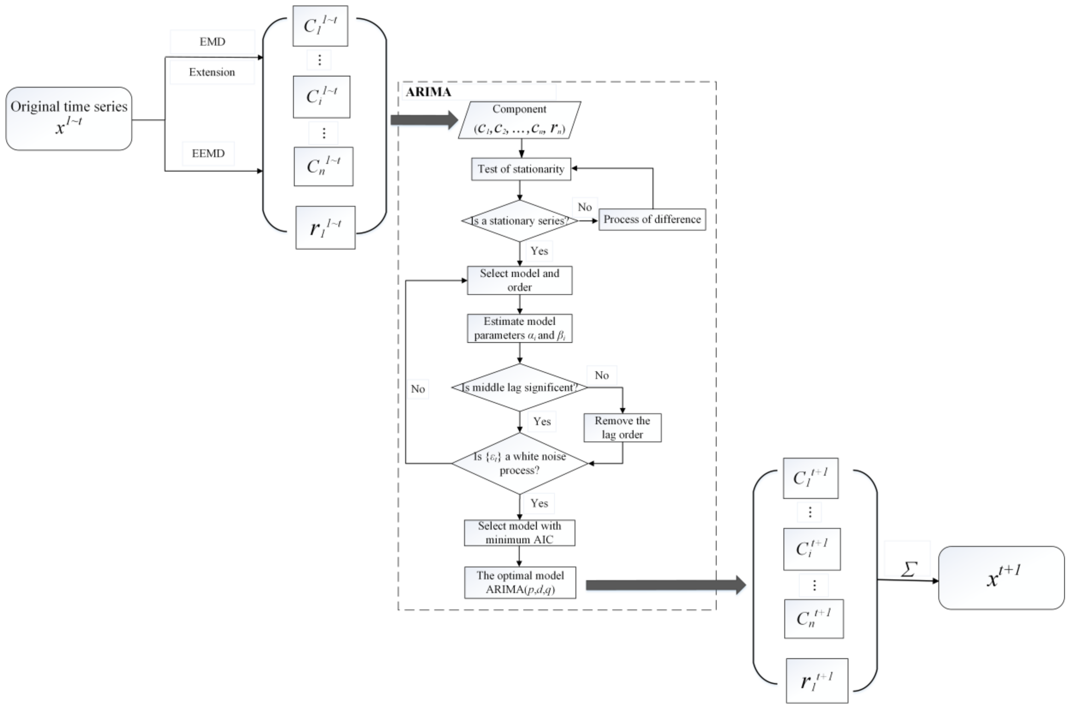
In order to improve prediction accuracy, the original average ten-day time series are firstly decomposed into several components with different time scales by EMD or EEMD to obtain stationary sub-sequences, each of which is then predicted one-time step ahead by ARIMA, and the combination of these predicted sub-sequences is taken as the prediction value of the original stream flow for the next time step. Figure 1 shows the flowchart of the hybrid EMD/EEMD-ARIMA models above, and the implementation steps are illustrated below:
- 1.
- Let { ∈ X: t = 1, 2, …, N} denote the original average ten-day hydrological time series.
- 2.
- Divide the time series into calibration datasets { ∈ X: t = 1, 2, …, k} and validation datasets { ∈ X: t = k, k + 1, …, n}.
- 3.
- Decompose the time series by EMD and EEMD to obtain IMFs and residual .
- 4.
- Establish appropriate ARIMA models with appropriate parameters for each IMF and residual. Box and Jenkins [50] set the standard for modeling stationary time series by using ARIMA model. The detailed modeling process of ARIMA model mainly includes: ① Let { ∈ Z: t = 1, 2, …, N} denotes the time series that need to be modeled; ② Check whether satisfies the condition of stationary time series by the unit root test. If the time series is a non-stationary time series, that means there are unit roots in the time series, and the original time series needs to be differentiated to obtain a stationary time series ; ③ Select appropriate models (AR model, MA model or ARMA model), and the lag order can be based on an autocorrelation (AC) function and the partial correlation (PAC) function of the stationary time series ; ④ Estimate the parameters in the model. If some of the parameters in the middle lag are too small, the parameters are not significant (the significance level used in this study is 5%); these lag orders need to be removed from the model; ⑤ Residuals of the model are determined to be white noise or not; if residual sequences are white noise, the autocorrelation coefficients of non-zero lag are all zero. This can be tested by the Q statistic (shown in Equation (13)) proposed by Box et al. [51] and Ljung et al. [52].where is the sample’s autocorrelation coefficient, and if the sample size is large enough, . The Q-statistic approximately obeys a distribution and the degree of freedom is s. If the residual sequence is not white noise, then the model needs to be improved; ⑥ The model with the minimum AIC (Akaike Information Criterion) [53] is chosen as the optimal model from many models which satisfy the conditions in steps ②–⑤).
- 5.
- Use the candidate models ARIMA (p, d, q) to compute one-time step ahead forecast across all the components of EMD/EEMD which would result in component forecasts (). The prediction of one time step ahead is the sum of each component prediction (shown in Equation (11)).In order to be fairly compared with the ARIMA model, the prediction of the hybrid model is also carried out at one-time step ahead every time.
- 6.
- Record observed data for one-time step ahead. Add these data to and decompose the updated calibration datasets. Repeat steps 3–5 until obtain all components are forecast for the complete original time series.
2.5. Verification Strategy
In this paper, the original average ten-day streamflow of six years is decomposed into several stationary subsequences. An appropriate ARIMA model is built for each subsequence to get one-time step ahead predictions. The combinations of these predictions are taken as the predictive result of the original streamflow. Such a rolling forecast continues with additional observations, and we finally get the average ten-day streamflow forecasts for the next five years.
The predictive performance of different models is estimated by comparing the observation and prediction. The Root Mean Square Error (RMSE), Normalized Root Mean Square Error (NRMSE), Mean Absolute Percentage Error (MAPE), Mean Absolute Error (MAE) and correlation coefficient (R) are used to estimate the performance of hybrid models, as defined in Equations (12)–(15). RMSE can assess the fitting degree between the predicted and the observed data with a high value, and MAE estimates the fitness of moderate streamflow from a more balanced perspective [40]. MAPE is used to evaluate the fitness between the predicted and the observed data with a moderate value, and R shows the degree of linear correlation between the prediction and the observed data.
where N denotes the number of datasets; represents the observed data; and represents the forecasting; represents the maximum of observed data; represents the minimum of observed data; represents the average of observed data and represents the average of forecasting.
3. Case Study
3.1. Study Case
In this study, the data are from Yellow River hydrological website. The Yellow River ranks as the fifth longest river in the world and the second longest river in China with the total length of 5464 km. The source region of the yellow river provides a large amount of water resources for northwest China, accounting for 34.5% of the whole average annual inflow in the Yellow River basin. Tangnaihai hydrological station is the control station of the source region of the Yellow River, the basin area above which is about 121,972 km2, taking up 16.2% of the total Yellow River basin area.
Tangnaihai hydrological station is also the upstream control station of the Longyangxia reservoir, the first large-scale reservoir on the Yellow River, as shown in Figure 2. The operation of the Longyangxia reservoir affects the whole Yellow River downstream, which depends greatly on the inflow. Thus, the accurate long-term prediction of the hydrological time series at Tangnaihai station becomes particularly important.
In this study, average ten-day streamflow data of the Tangnaihai station of six years are used to predict the streamflow of the following year using the proposed hybrid models, and the historical record of the predicted year is taken to evaluate the predictive accuracy. The prediction is executed for 5 years from 2013 to 2017, i.e., the average ten-day data from the year 2007 to 2012 is used to predict the flow of 2013, the data from 2008 to 2013 is used to predict the flow of 2014, and such prediction continues for 5 years.
3.2. Results
Both the hybrid EMD/EEMD-ARIMA model and the ARIMA model are applied to predict the streamflow time series of Tangnaihai hydrological station. In this case, the standard proposed by Box and Jenkins [50] is considered as the criteria of building candidate models for all components and the order of ARIMA models is determined by Auto Correlation function (ACF) and Partial Auto Correlation Function (PACF) plots, as shown in Figure 3. Figure 3 indicates that these components are neither pure AR nor MA models but ARMA models. Since the forecast lead time is one year with ten-day interval, and there are 36 time steps in total, the amplitude of orders was tested in the range of 1~36, and the model with minimum AIC value is selected for forecasting of each component.
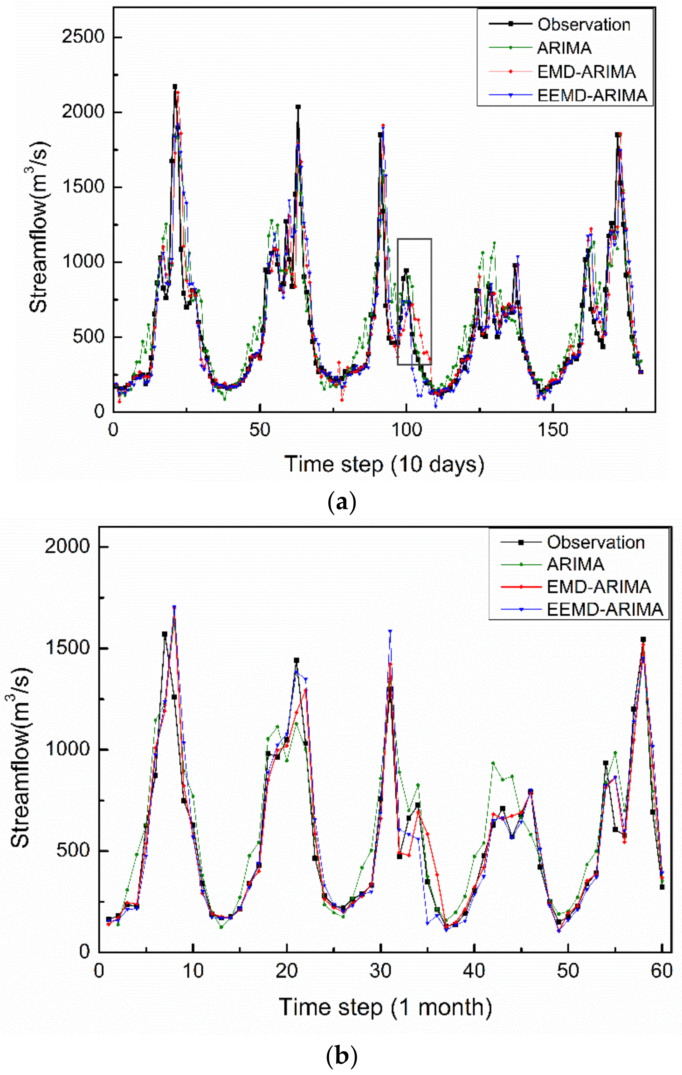
The ten-day average and monthly streamflow predictions resulting from the proposed EMD/EEMD-ARIMA method and ARIMA model are compared in Figure 4. Figure 4a presents the results of predictions with different methods illustrated in Section 2, taking ten days as the time step. The black line shows the historical records of the streamflow at the Tangnaihai station, while the green, blue, and red lines are the predictive results with ARIMA, EMD-ARIMA, and EEMD-ARIMA models, respectively. The corresponding monthly statistics are shown in Figure 4b.
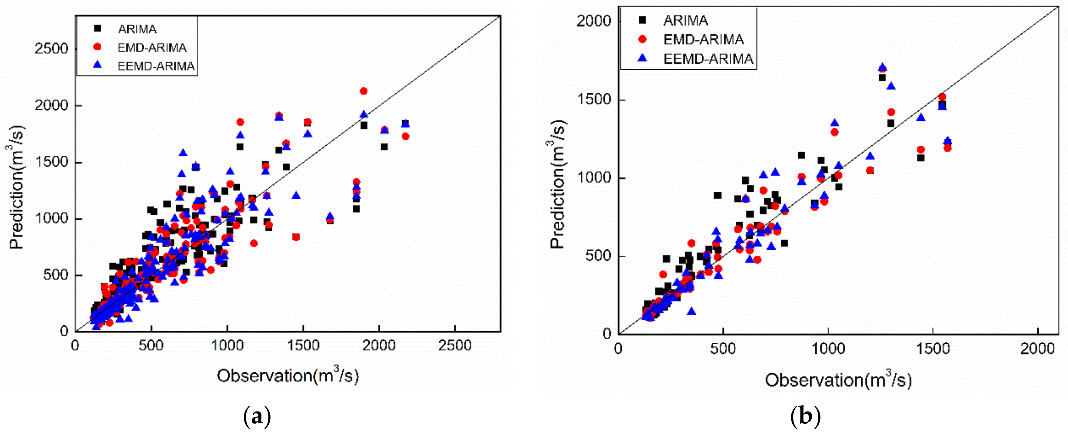
Figure 5 shows the scatter plots of the predicted and observed streamflow of ten-day average and monthly data individually. The black square, red circle and blue triangle represent the predictive value corresponding to observation by ARIMA model, EMD-ARIMA, and EEMD-ARIMA hybrid models, respectively. The closer to the black line, the more accurate the predictions are.
It can be seen from both Figure 4 and Figure 5 that the prediction by the ARIMA model overestimates the observations. The reason lies in the continuity of the trends, which can be understood as the inertial property of the forecast when using ARIMA models. For ARIMA models, the historical data nearest to the current stage has the greatest impact on the prediction. If the historical data rise suddenly right before the peak value, it cannot be foreseen by the ARIMA model, and thus the peak value will be underestimated; but if the rise is slow and steady, the rising trend will be expected to continue after the peak by ARIMA model, and the predictions are thus higher than the observations. Basically, the increase of the streamflow is gradual, and thus there appear many overestimations for the ARIMA model. The predictions of both the EMD-ARIMA and EEMD-ARIMA hybrid models accord with the observation much better compared to the ARIMA model in Figure 4, and the scatter plots in Figure 5 of the hybrid models also distribute evenly on both sides of the observation line. Nevertheless, the lag resulting from the dependence on the previous value in ARIMA method maybe still appear in the hybrid models, such as the first peak prediction in Figure 4b. Although EEMD overcomes the mode mixing problem resulting from signal intermittency, the introduction of the white noises may leads to inaccuracy, or even mis-judgement of the change tendency, as shown in the grey rectangle in Figure 4. With proper disposal of the end point problem for EMD, the EMD-ARIMA hybrid model performs well to predict long-term flow with high accuracy.
Table 1 shows the statistical accuracy of the predictions by different models, indicated by MAPE, RMSE, MAE and R. The smaller the values of MAPR, RMSE, MAE, the more accurate the predictions. The maximum value of R is 1, and a higher value of R indicates a better fit between prediction and observation.
Table 1 indicates that the EMD-ARIMA hybrid model outperforms both EEMD-ARIMA and ARIMA models with the smallest MAPE, RMSE, and MAE for both ten-day and monthly prediction. The fitting degree, R, of the EMD-ARIMA model is above 0.9 for the ten-day prediction and as high as 0.95 for the monthly prediction. Even for the EEMD-ARIMA model, R is 0.89 and 0.95 for ten-day and monthly prediction, respectively. The correlation coefficients R of the monthly prediction by both EMD-ARIMA and EEMD-ARIMA hybrid model are both higher than the previous studies of Zhu et al. [40], Zhang et al. [44], and Kisi et al. [45], which use rainfall and runoff data, or monthly data directly. The performance of RMSE, MAPE, MAE and R of the monthly prediction is higher than that of the ten-day prediction in all models. The reason for the difference is that some errors in the prediction with a small time interval might be smoothed in the statistics for the longer time interval.
Forecast skill can also be indicated by skill score , as shown in Equation (16):
where is the accuracy measure achieved by perfect forecast which equals the observed value; A is the value of the accuracy measure that can be obtained by the proposed method; is the accuracy of a set of reference forecast. In this study, we calculate skill score based on MAE and choose the results from the ARIMA model as the reference. If , the skill score get the maximum value of 100%; while if , then = 0%, which indicates that there is no improvements of the proposed method comparing with the reference forecast. If < 0%, the estimated forecast is inferior to the reference forecast.
The skill score in Table 2 verifies the superiority of the proposed EMD/EEMD-ARIMA models compared to the ARIMA model, indicating that the decomposition methods are able to exploit the comprehensive information from the original data set to improve the prediction.
4. Discussion and Conclusions
In this study, hybrid models coupling EMD/EEMD and ARIMA are proposed to forecast non-stationary monthly streamflow time series. The basic idea is to decompose time series into several components and model them by ARIMA models for separate predictions, the reconfiguration of which results in one time step ahead time series predictions. The proposed hybrid methods are compared with the ARIMA model, and four statistical performance evaluation measures (MAPE, RMSE, MAE and R) are adopted to evaluate various models. For sufficient information mining, we used ten-day average data instead of monthly data as most of the long-term forecast studies. In the existing study by Zhang et al. [44], monthly data of over 50 years were used for prediction, and the MAPE was 0.22 and 0.19, respectively, for the two stations they selected, and the R was 0.602 and 0.519, respectively. While in this study, ten-day average data of only 6 years were used, and the MAPE of monthly prediction was 0.127, and 0.137 for the EMD-ARIMA, and EEMD-ARIMA models, respectively, and the R was also as high as 0.950 for both of the models. The comparison indicates that the time sequence with a smaller time interval contains more detailed information which is helpful for prediction, and the decomposition methods are effective for mining such information. The main findings of this study include: (1) the EMD/EEMD-ARIMA models can improve the predictive accuracy of stream flow forecasting compared to the original ARIMA model, only using flow data; (2) the decomposition by EMD and EEMD is able to exploit the information hidden in the time series with a small time interval, which helps to improve the monthly prediction; and (3) the boundary problem affects the decomposition results of EMD greatly. With the extension disposal of the end points for EMD, the hybrid EMD-ARIMA model results in monthly predictions with RMSE, MAPE, MAE and R of 121.26, 0.13, 74.77, and 0.95, respectively, which are better than the previous publications on flow prediction with rainfall and runoff data, or with monthly data directly.
Author Contributions
Conceptualization, J.Q. and F.-F.L.; Methodology, Z.-Y.W. and F.-F.L.; Validation, Z.-Y.W. and F.-F.L.; Formal Analysis, Z.-Y.W. and F.-F.L.; Investigation, J.Q. and F.-F.L.; Resources, F.-F.L.; Writing-Original Draft Preparation, Z.-Y.W.; Writing-Review & Editing, F.-F.L.; Supervision, F.-F.L.; Funding Acquisition, F.-F.L.
Funding
This research was founded by the National Key R&D Program of China, grant numbers 2017YFC0403600, 2017YFC0403602.
Conflicts of Interest
The authors declare no conflict of interest.
References
- Yang, L.; Tian, F.; Sun, Y.; Yuan, X.; Hu, H. Attribution of hydrologic forecast uncertainty within scalable forecast windows. Hydrol. Earth Syst. Sci. 2014, 18, 775–786. [Google Scholar] [CrossRef] [Green Version]
- Seo, Y.; Kim, S.; Kisi, O.; Singh, V.P. Daily water level forecasting using wavelet decomposition and artificial intelligence techniques. J. Hydrol. 2015, 520, 224–243. [Google Scholar] [CrossRef]
- He, Z.; Wen, X.; Liu, H.; Du, J. A comparative study of artificial neural network, adaptive neuro fuzzy inference system and support vector machine for forecasting river flow in the semiarid mountain region. J. Hydrol. 2014, 509, 379–386. [Google Scholar] [CrossRef]
- Borga, M.; Stoffel, M.; Marchi, L.; Marra, F.; Jakob, M. Hydrogeomorphic response to extreme rainfall in headwater systems: Flash floods and debris flows. J. Hydrol. 2014, 518, 194–205. [Google Scholar] [CrossRef]
- Strauch, M.; Bernhofer, C.; Koide, S.; Volk, M.; Lorz, C.; Makeschin, F. Using precipitation data ensemble for uncertainty analysis in SWAT streamflow simulation. J. Hydrol. 2012, 414, 413–424. [Google Scholar] [CrossRef]
- Ralph, F.M.; Coleman, T.; Neiman, P.J.; Zamora, R.J.; Dettinger, M.D. Observed impacts of duration and seasonality of atmospheric-river landfalls on soil moisture and runoff in coastal Northern California. J. Hydrometeorol. 2013, 14, 443–459. [Google Scholar] [CrossRef]
- Hanna, E.; Jones, J.M.; Cappelen, J.; Mernild, S.H.; Wood, L.; Steffen, K.; Huybrechts, P. The influence of North Atlantic atmospheric and oceanic forcing effects on 1900–2010 Greenland summer climate and ice melt/runoff. Int. J. Climatol. 2013, 33, 862–880. [Google Scholar] [CrossRef]
- Rosenberg, E.A.; Clark, E.A.; Steinemann, A.C.; Lettenmaier, D.P. On the contribution of groundwater storage to interannual streamflow anomalies in the Colorado River basin. Hydrol. Earth Syst. Sci. 2013, 17. [Google Scholar] [CrossRef]
- Sinha, T.; Sankarasubramanian, A.; Mazrooei, A. Decomposition of sources of errors in monthly to seasonal streamflow forecasts in a rainfall-runoff regime. J. Hydrometeorol. 2014, 15, 2470–2483. [Google Scholar] [CrossRef]
- Aqil, M.; Kita, I.; Yano, A.; Nishiyama, S. A comparative study of artificial neural networks and neuro-fuzzy in continuous modeling of the daily and hourly behaviour of runoff. J. Hydrol. 2007, 337, 22–34. [Google Scholar] [CrossRef]
- Kalra, A.; Miller, W.P.; Lamb, K.W.; Ahmad, S.; Piechota, T. Using large-scale climatic patterns for improving long lead time streamflow forecasts for Gunnison and San Juan River Basins. Hydrol. Process. 2013, 27, 1543–1559. [Google Scholar] [CrossRef]
- Verkade, J.S.; Brown, J.D.; Reggiani, P.; Weerts, A.H. Post-processing ECMWF precipitation and temperature ensemble reforecasts for operational hydrologic forecasting at various spatial scales. J. Hydrol. 2013, 501, 73–91. [Google Scholar] [CrossRef]
- Aubert, A.H.; Tavenard, R.; Emonet, R.; de Lavenne, A.; Malinowski, S.; Guyet, T.; Quiniou, R.; Odobez, J.M.; Merot, P.; Gascuel-Odoux, C. Clustering flood events from water quality time series using Latent Dirichlet Allocation model. Water Resour. Res. 2013, 49, 8187–8199. [Google Scholar] [CrossRef] [Green Version]
- Wang, W.C.; Chau, K.W.; Qiu, L.; Chen, Y.B. Improving forecasting accuracy of medium and long-term runoff using artificial neural network based on EEMD decomposition. Environ. Res. 2015, 139, 46–54. [Google Scholar] [CrossRef] [PubMed]
- Gulhane, P.; Menezes, B.; Reddy, T.; Shah, K.; Soman, S.A. Forecasting using decomposition and combinations of experts. In Proceedings of the 2005 International Conference on Artificial Intelligence (ICAI ‘05), Las Vegas, NV, USA, 27–30 June 2005; Arabnia, H.R., Joshua, R., Eds.; CSREA Press: Athens, Greece, 2005; pp. 67–73. ISBN 1-932415-68-8. [Google Scholar]
- Kalteh, A.M. Monthly river flow forecasting using artificial neural network and support vector regression models coupled with wavelet transform. Comput. Geosci. 2013, 54, 1–8. [Google Scholar] [CrossRef]
- Dehghani, M.; Saghafian, B.; Saleh, F.N.; Farokhnia, A.; Noori, R. Uncertainty analysis of streamflow drought forecast using artificial neural networks and Monte-Carlo simulation. Int. J. Climatol. 2014, 34, 1169–1180. [Google Scholar] [CrossRef]
- Dariane, A.B.; Azimi, S. Forecasting streamflow by combination of a genetic input selection algorithm and wavelet transforms using ANFIS models. Hydrol. Sci. J. 2016, 61, 585–600. [Google Scholar] [CrossRef]
- Shi, B.; Hu, C.H.; Yu, X.H.; Hu, X.X. New fuzzy neural network-Markov model and application in mid- to long-term runoff forecast. Hydrol. Sci. J. 2016, 61, 1157–1169. [Google Scholar] [CrossRef]
- Lohani, A.K.; Kumar, R.; Singh, R.D. Hydrological time series modeling: A comparison between adaptive neuro-fuzzy, neural network and autoregressive techniques. J. Hydrol. 2012, 442, 23–35. [Google Scholar] [CrossRef]
- Dong, S.; Chi, K.; Zhang, Q.Y.; Zhang, X.D. The application of a Grey Markov Model to forecasting annual maximum water levels at hydrological stations. J. Ocean Univ. China 2012, 11, 13–17. [Google Scholar] [CrossRef]
- Wu, J.S.; Han, J.; Annambhotla, S.; Bryant, S. Artificial neural networks for forecasting watershed runoff and stream flows. J. Hydrol. Eng. 2005, 10, 216–222. [Google Scholar] [CrossRef]
- Chang, F.J.; Chiang, Y.M.; Chang, L.C. Multi-step-ahead neural networks for flood forecasting. Hydrol. Sci. J. 2007, 52, 114–130. [Google Scholar] [CrossRef] [Green Version]
- Sudheer, C.; Maheswaran, R.; Panigrahi, B.K.; Mathur, S. A hybrid SVM-PSO model for forecasting monthly streamflow. Neural Comput. Appl. 2013, 24, 1381–1389. [Google Scholar] [CrossRef]
- Nanda, T.; Sahoo, B.; Beria, H.; Chatterjee, C. A wavelet-based non-linear autoregressive with exogenous inputs (WNARX) dynamic neural network model for real-time flood forecasting using satellite-based rainfall products. J. Hydrol. 2016, 539, 57–73. [Google Scholar] [CrossRef]
- Armstrong, J.S. Combing forecast—The end of the beginning or the beginning of the end. Int. J. Forecast. 1989, 5, 585–588. [Google Scholar] [CrossRef]
- Temraz, H.K.; Salama, M.M.A.; Quintana, V.H. Application of the decomposition technique for forecasting the load of a large electric power network. IEE Proc. Gener. Transm. Distrib. 1996, 143, 13–18. [Google Scholar] [CrossRef]
- Zou, H.; Yang, Y.H. Combining time series models for forecasting. Int. J. Forecast. 2004, 20, 69–84. [Google Scholar] [CrossRef] [Green Version]
- Hibon, M.; Evgeniou, T. To combine or not to combine: Selecting among forecasts and their combinations. Int. J. Forecast. 2005, 21, 15–24. [Google Scholar] [CrossRef]
- Wu, C.L.; Chau, K.W.; Fan, C. Prediction of rainfall time series using modular artificial neural networks coupled with data-preprocessing techniques. J. Hydrol. 2010, 389, 146–167. [Google Scholar] [CrossRef] [Green Version]
- Lin, C.S.; Chiu, S.H.; Lin, T.Y. Empirical mode decomposition-based least squares support vector regression for foreign exchange rate forecasting. Econ. Model. 2012, 29, 2583–2590. [Google Scholar] [CrossRef]
- Nourani, V.; Hosseini Baghanam, A.; Adamowski, J.; Kisi, O. Applications of hybrid wavelet–Artificial Intelligence models in hydrology: A review. J. Hydrol. 2014, 514, 358–377. [Google Scholar] [CrossRef]
- Nourani, V.; Komasi, M.; Alami, M.T. Hybrid wavelet–genetic programming approach to optimize ANN modeling of rainfall–runoff process. J. Hydrol. Eng. 2012, 17, 724–741. [Google Scholar] [CrossRef]
- Badrzadeh, H.; Sarukkalige, R.; Jayawardena, A.W. Improving ANN-based short-term and long-term seasonal river flow forecasting with signal processing techniques. River Res. Appl. 2016, 32, 245–256. [Google Scholar] [CrossRef]
- Liu, Y.Q.; Brown, J.; Demargne, J.; Seo, D.J. A wavelet-based approach to assessing timing errors in hydrologic predictions. J. Hydrol. 2011, 397, 210–224. [Google Scholar] [CrossRef]
- Maheswaran, R.; Khosa, R. Comparative study of different wavelets for hydrologic forecasting. Comput. Geosci. 2012, 46, 284–295. [Google Scholar] [CrossRef]
- Huang, N.E.; Shen, Z.; Long, S.R.; Wu, M.L.C.; Shih, H.H.; Zheng, Q.N.; Yen, N.C.; Tung, C.C.; Liu, H.H. The empirical mode decomposition and the Hilbert spectrum for nonlinear and non-stationary time series analysis. Proc. R. Soc. A Math. Phys. Eng. Sci. 1998, 454, 903–995. [Google Scholar] [CrossRef]
- Huang, N.E.; Wu, Z. A review on Hilbert-Huang transform: Method and its applications to geophysical studies. Rev. Geophys. 2008, 46. [Google Scholar] [CrossRef] [Green Version]
- Lee, T.; Ouarda, T.B.M.J. Long-term prediction of precipitation and hydrologic extremes with nonstationary oscillation processes. J. Geophys. Res. 2010, 115. [Google Scholar] [CrossRef] [Green Version]
- Zhu, S.; Zhou, J.; Ye, L.; Meng, C. Streamflow estimation by support vector machine coupled with different methods of time series decomposition in the upper reaches of Yangtze River, China. Environ. Earth Sci. 2016, 75. [Google Scholar] [CrossRef]
- Wu, Z.; Huang, N.E. Ensemble empirical mode decomposition: A noise-assisted data analysis method. Adv. Adapt. Data Anal. Theory Appl. 2009, 1, 1–41. [Google Scholar] [CrossRef]
- Chiew, F.H.S.; Peel, M.C.; Amirthanathan, G.E.; Pegram, G.G.S. Identification of oscillations in historical global streamflow data using empirical mode decomposition. In Regional Hydrological Impacts of Climatic Change—Hydroclimatic Variability; Franks, S., Wagener, T., Bogh, E., Gupta, H.V., Bastidas, L., Nobre, C., Galvao, C.D.O., Eds.; International Association Hydrological Sciences: Wallingford, UK, 2005; Volume 296, pp. 53–62. ISBN 978-1-901502-13-8. [Google Scholar]
- Zhang, H.; Singh, V.P.; Wang, B.; Yu, Y. CEREF: A hybrid data-driven model for forecasting annual streamflow from a socio-hydrological system. J. Hydrol. 2016, 540, 246–256. [Google Scholar] [CrossRef]
- Zhang, X.; Peng, Y.; Zhang, C.; Wang, B. Are hybrid models integrated with data preprocessing techniques suitable for monthly streamflow forecasting? Some experiment evidences. J. Hydrol. 2015, 530, 137–152. [Google Scholar] [CrossRef]
- Kisi, O.; Latifoğlu, L.; Latifoğlu, F. Investigation of empirical mode decomposition in forecasting of hydrological time series. Water Res. Manag. 2014, 28, 4045–4057. [Google Scholar] [CrossRef]
- Di, C.L.; Yang, X.H.; Wang, X.C. A four-stage hybrid model for hydrological time series forecasting. PLoS ONE 2014, 9, e104663. [Google Scholar] [CrossRef] [PubMed]
- Zhao, X.; Chen, X. Auto regressive and ensemble empirical mode decomposition hybrid model for annual runoff forecasting. Water Res. Manag. 2015, 29, 2913–2926. [Google Scholar] [CrossRef]
- Hou, H.S.; Andrews, H.C. Cubic-splines for image interpolation and digital filtering. IEEE Trans. Acoust. Speech Signal Process. 1978, 26, 508–517. [Google Scholar]
- Valipour, M.; Banihabib, M.E.; Behbahani, S.M.R. Comparison of the ARMA, ARIMA, and the autoregressive artificial neural network models in forecasting the monthly inflow of Dez dam reservoir. J. Hydrol. 2013, 476, 433–441. [Google Scholar] [CrossRef]
- Box, G.E.P.; Jenkins, G. Time series analysis, forecasting and control. In Time Series Analysis, Forecasting and Control; INSPEC:209917; Holden-Day: San Francisco, CA, USA, 1970; pp. 19–553. [Google Scholar]
- Box, G.E.P.; Pierce, D.A. Distribution of residual autocorrelations in autoregressive-integrated moving average time series models. J. Am. Stat. Assoc. 1970, 65, 1509–1526. [Google Scholar] [CrossRef]
- Ljung, G.M.; Box, G.E.P. Measure of lack of fit in time-series models. Biometrika 1978, 65, 297–303. [Google Scholar] [CrossRef]
- Akaike, H. Bayesian-analysis of minimum AIC procedure. Ann. Inst. Stat. Math. 1978, 30, 9–14. [Google Scholar] [CrossRef]
Figure 1.
Flowchart of the EMD/EEMD-ARIMA hybrid method for time series prediction.

Figure 2.
Study area.

Figure 3.
(a) Autocorrelation (AC) and (b) partial autocorrelation (PAC) plots for streamflow time series.
Figure 3.
(a) Autocorrelation (AC) and (b) partial autocorrelation (PAC) plots for streamflow time series.


Figure 4.
Streamflow prediction by proposed hybrid methods from the year 2013 to 2017 (a) with a time step of (a) ten days; (b) one month.
Figure 4.
Streamflow prediction by proposed hybrid methods from the year 2013 to 2017 (a) with a time step of (a) ten days; (b) one month.

Figure 5.
Comparison of deviation between streamflow prediction and historical data by proposed hybrid methods from the year 2013 to 2017 with a time step of (a) ten days; (b) one month.
Figure 5.
Comparison of deviation between streamflow prediction and historical data by proposed hybrid methods from the year 2013 to 2017 with a time step of (a) ten days; (b) one month.


Table 1.
Statistical results of the predictive accuracy.
| Model | Ten-Day Prediction | Monthly Prediction | ||||||
|---|---|---|---|---|---|---|---|---|
| MAPE | RMSE (m3/s) | MAE (m3/s) | R | MAPE | RMSE (m3/s) | MAE (m3/s) | R | |
| ARIMA | 0.284 | 214.75 | 143.67 | 0.870 | 0.232 | 153.21 | 111.60 | 0.930 |
| EMD-ARIMA | 0.186 | 182.00 | 109.40 | 0.903 | 0.127 | 121.260 | 74.77 | 0.950 |
| EEMD-ARIMA | 0.194 | 196.44 | 117.71 | 0.894 | 0.137 | 129.28 | 80.90 | 0.950 |
Table 2.
Forecast skill score of hybrid models.
| Model | Ten-Day Prediction | Monthly Prediction |
|---|---|---|
| Skill Score | Skill Score | |
| EMD-ARIMA | 0.239 | 0.330 |
| EEMD-ARIMA | 0.181 | 0.275 |
© 2018 by the authors. Licensee MDPI, Basel, Switzerland. This article is an open access article distributed under the terms and conditions of the Creative Commons Attribution (CC BY) license (http://creativecommons.org/licenses/by/4.0/).
Share and Cite
MDPI and ACS Style
Wang, Z.-Y.; Qiu, J.; Li, F.-F. Hybrid Models Combining EMD/EEMD and ARIMA for Long-Term Streamflow Forecasting. Water 2018, 10, 853. https://doi.org/10.3390/w10070853
AMA Style
Wang Z-Y, Qiu J, Li F-F. Hybrid Models Combining EMD/EEMD and ARIMA for Long-Term Streamflow Forecasting. Water. 2018; 10(7):853. https://doi.org/10.3390/w10070853
Chicago/Turabian StyleWang, Zhi-Yu, Jun Qiu, and Fang-Fang Li. 2018. "Hybrid Models Combining EMD/EEMD and ARIMA for Long-Term Streamflow Forecasting" Water 10, no. 7: 853. https://doi.org/10.3390/w10070853
Note that from the first issue of 2016, this journal uses article numbers instead of page numbers. See further details here.