Impact of Infiltration Process Modeling on Soil Water Content Simulations for Irrigation Management

Abstract

The uncertainty in a hydrological model, due to its structure or implemented input parameters, affects the accuracy of simulations that are usually used for important applications such as drought predictions, flood risk assessment, irrigation scheduling, ground water recharge and contamination. Several models describing soil infiltration processes have been developed. Some are analytical, while others implement numerical solutions of the Richards’ equation. The objective of this work was to assess the impact of infiltration process modeling on soil water content simulations. For this study, different infiltration models were included within FEST-WB (Flash Flood Event-based Spatially-distributed rainfall-runoff Transformations-Water Balance) distributed hydrological model (SCS-CN, Green and Ampt, Philip and Ross solution). Performances of implemented infiltration models in simulating soil water content were evaluated against observations acquired in the experimental site located in a maize field in northern Italy. Soil water content was monitored together with continuous measurements of meteorological data. A sensitivity analysis was performed to assess the most important parameters governing infiltration process in the different models tested. A comparison of soil water content simulations show that Ross solution allowed the description of soil moisture variation along the vertical, but simpler lumped models provide sufficient accuracy when properly calibrated.

1. Introduction

Infiltration is defined as the water movement from the ground surface into the soil [1]. The rate of water flow through the soil is directly related to many hydrological processes: ground water recharge, water supply to plants, heat and solute transport, erosion and runoff [2]. In addition, the infiltration is controlled by several factors: soil texture and structure, initial water content, rainfall or irrigation application rates, etc. [3]. This has made the description of water flow in the vadose zone, which is quite difficult as compared to the saturated zone [4], one of the challenging tasks that modelers may face when developing hydrological models.

Modeling the infiltration process has gained great interest from soil and water scientists [5]. Several infiltration models exist in the literature that exhibit different levels of accuracy. These models are usually based on Richards’ equation [6,7], which provides an appropriate tool to describe the infiltration process with a detailed description of the flow and water distribution within the soil profile [8]. Numerical solutions based on finite difference, finite element or boundary element techniques [9] have been used to solve Richards’ equation. Due to the non-linearity of the described process as well as the high soil hydraulic parameters requirements, the use of numerical solutions is considered as time consuming with some stability problems [8]. Despite the progress made for developing efficient numerical schemes joined with faster computers, the use of such numerical methods is still time consuming when implemented for large study areas [10].

On the other hand, because of the limitations of commonly implemented numerical solutions, numerous simplifications have been suggested to model the infiltration process. Accordingly, various classification criteria of infiltration models exist [11]. These models are commonly categorized into empirical, semi-empirical and physically based [12]. Empirical models are formulated as a simple equation, derived from actual field measured infiltration data through curve fitting [11]. Examples of these models are: Kostiatov [13], SCS-CN (US Department of Agriculture Soil Conservation Service, [14]), Huggins and Monke [15], Collis-George [16], etc. Many existing hydrological models in the literature are based on these empirical models, in particular the SCS-CN such as ANSWERS [17], EPIC [18], SWAT [19], etc.

Many semi-empirical or approximate models exist such as Philip [20], Smith and Parlange [21], Green and Ampt [22], etc. These models allow a simplification of this process through some assumptions made either for soil hydraulic properties or for the boundary conditions [7]. Approximate solutions of Richards’ equation are restricted by some conditions of application, for example: ponding surface, dry profile, constant diffusivity or constant water flux in the surface [23]. On the contrary, numerical solutions have been considered as more efficient to solve the Richards’ equation under different field conditions [24].

Recently, a new fast non-iterative solution for the non-linear 1D Richards’ equation has been proposed by Ross [10]. Several researchers have considered Ross solution as a numerical solution [10,23,24]. This solution allowed overcoming the limitations of other commonly used numerical solutions [23]. Ross model performances have been tested against several models. Varado et al. [23] assessed the efficiency of Ross model by comparing it at a first step with two analytical solutions and at a second step with SIPAT model. The results of this study showed that Ross solution [10] is a robust and accurate solution while a finer discretization is required close to soil surface to improve the results of cumulative infiltration. Crevoisier et al. [24] compared within their study the Ross model with a finite element based Hydrus 1D model to evaluate the accuracy, computing time and convergence quality. This comparison was carried out considering different soil types, different initial water content and grid types. Results of this study showed that Ross model gave better results than Hydrus 1D model in terms of simulation quality and computing time while this latter presented some convergence problems. Recently, Tinet et al. [8] developed a decision tool based on Ross solution. The model proved good efficiency as compared with the TEC model [25] with 90% agreements in the results. Adding to that, Ross model can provide good results under large temporal and spatial scales [24]

The advances in developing sophisticated models and the implemented procedures for model parameterization obviously increased models simulations accuracy [26]. Nevertheless, the suitability of these models for real world conditions should be assessed [12]. The evaluation of model performances is based on the estimate of closeness of model simulations to observations [27]. The inter-comparison of different models allowed affirming their points of strength and weakness [28]. The selection of the equation to be implemented to describe a given process within a model can influence the results of model simulation. Hence, this step should be carried out carefully to limit uncertainties, originating from a process representation, on model predictions.

The current study aims at assessing the effect of infiltration process modeling on soil water content simulations accuracy for irrigation water management. To this aim, different infiltration models were included within the FEST-WB (Flash Flood Event-based Spatially-distributed-rainfall-runoff Transformations-Water Balance), a distributed hydrological model developed at Politecnico di Milano since 1990. As a first step, Green and Ampt (GA), Philip and the modified curve number (SCS-CN) were included within FEST-WB. Then, Ross model was implemented using Brooks and Corey [29] and Van Genuchten [30] soil water retention curve models. For this study, we limited our focus to a homogeneous soil profile.

The first objective of this study was therefore to identify the most important parameters governing infiltration process within the different implemented models through a performed sensitivity analysis. The second objective was to evaluate the performances of implemented models against observations acquired in the experimental study site, an agricultural field, where soil water content was monitored together with continuous measurements of meteorological data. The third objective was to assess the effect of the selection of different infiltration models on the results of evaluation of an implemented irrigation scheduling.

2. Materials and Methods

2.1. Infiltration Models

2.1.1. The SCS-Curve Number

The SCS-curve number [14] is widely implemented for the calculation of surface runoff. According to this method, the infiltration is calculated as the difference between the precipitation and the runoff. SCS-CN method does not consider the rainfall intensity or duration; it only considers the total precipitation.

$$I=P_{tot}-R$$

(1)

$$R=\frac{{\left(P-I_a\right)}^2}{P-I_a+S}$$

(2)

With

$$I_a=0.2S$$

(3)

where I is the total infiltration [L], P is the precipitation [L], R is the runoff [L], S is the maximum retention capacity [L], and I_a is the initial abstraction. S and CN are related by:

$$CN=\frac{1000}{10+S}$$

(4)

The CN parameter values were derived from the curves of the plotted relationship between the rainfall and the runoff. CN is mainly related to the land use. The CN value is adjusted according to the antecedent moisture conditions. In particular, CN I stands for dry soil moisture conditions AMC I, CN II stands for soil moisture conditions (AMC II) of the previous 5 days and CN III stands for wet soil moisture conditions AMC III. The SCS-CN approach has been subjected to several modifications to be adopted for various land uses and climatic conditions [31]. Many researchers have proposed a modified version of the SCS-CN for continuous simulations (e.g., [5,32,33]). The method proposed by Ravazzani et al. [34] was implemented within the FEST-WB model. According to this method, at each time step, S is calculated depending on the degree of the saturation of the soil.

$$S=S_1-\epsilon \left(S_1-S_3\right)$$

(5)

With

$$S_1=S\left(CN\left(I\right)\right)$$

(6)

$$S_3=S\left(CN\left(III\right)\right)$$

(7)

$${\epsilon }_t=\frac{{\theta }_t-{\theta }_r}{{\theta }_s-{\theta }_r}$$

(8)

where ε_t is the degree of saturation of the soil, θ_t is the actual water content at time t [L³/L³], θ_s is the saturated water content [L³/L³] and θ_r is the residual water content [L³/L³].

2.1.2. Philip’s Equation

Philip proposed a semi analytical solution [20] to solve the non-linear partial differential Richards equation [6]. The cumulative infiltration as expressed by Philip’s equation is approximated by

$$F\left(t\right)=S\times t^{\frac{1}{2}}+Kt$$

(9)

where S is a parameter called sorptivity, which is a function of the soil suction potential and K is the hydraulic conductivity [L/T]. The sorptivity is considered as capacity of the soil to uptake or release water. The sorptivity is computed based on Brooks and Corey model parameters according to the method proposed by Sivapalan et al. [35].

The time derivative of the cumulative infiltration is the infiltration rate [LT⁻¹]

$$f\left(t\right)=\frac{1}{2}S{t}^{\frac{-1}{2}}+K$$

(10)

When implemented within the FEST-WB model, the K(θ) is assumed to fit to Brooks and Corey model.

2.1.3. Green and Ampt

Green and Ampt model [22] is one of the widely used equations for the infiltration simulations within hydrological models, thanks to its simplicity and applicability for various soil textures under different conditions. This equation has been implemented for many practical engineering problems [36]. Examples of models implementing this solution are CLASS [37], HSPF [38], and SWAT [39]. This equation simplifies the infiltration process as a piston-like movement of a sharp wetting front and is considered as an analytical solution of Richards equation [40]. Green and Ampt is based on many assumptions [41]: the zone above the wetting front is considered as saturated, the water is ponded at a small depth (h₀) at the soil surface, the value of the suction head occurring at the wetting front is constant in time and depth with a uniform initial water content.

The Green Ampt equation as applied for steady rainfall condition and if the ponding depth is negligible is written as:

$$f=K[1+\frac{\left({\theta }_s-{\theta }_i\right)S_f}{F}]$$

(11)

$$F=k\times t+\left(S_f\left({\theta }_s-{\theta }_i\right)\times In\left[1+\frac{F}{\left({\theta }_s-{\theta }_i\right)S_f}\right]\right)$$

(12)

where K is the effective hydraulic conductivity [L/T], S_f is the effective suction at the wetting front [L], θ_s is the saturated water content [L³/L³], θ_i is the initial water content [L³/L³], F is the accumulated infiltration [L] and f is the infiltration rate [L/T]. Several modifications have been suggested to adapt Green and Ampt model to address situations beyond the assumptions of its development. Bouwer [42] extended this model to layered soil and non-uniform antecedent water content. Childs and Bybordi [43] implemented a heterogeneous soil profile with decreasing conductivity and developed a specified infiltration law according to the variability of the conductivity throughout the soil profile. To implement it within hydrological models for long simulation periods, it was required to modify the Green and Ampt for unsteady rainfall conditions. Mein and Larson [44] developed a method to detect the ponding time with infiltration into the soil using the Green and Ampt infiltration. The solution is based on pre-ponding phase during which the rainfall intensity is lower than infiltration capacity, than the ponding occurs when the rainfall rate starts to be equal or higher than the infiltration capacity. At the ponding time (t_p) [T], the cumulative infiltration (F_p) [[L] is equal to

$$F_p=f·t_p$$

(13)

where the ponding time is given by the following formula:

$$t_p=\frac{K.S_f\times \left({\theta }_s-{\theta }_i\right)}{f\left(f-k\right)}$$

(14)

The implemented Green and Ampt solution within the FEST-WB follows the method of Mein and Larson [44]. The suction head at the wetting front was defined according the soil textural class from Rawls et al. [45].

2.1.4. Ross (2003) Solution

Ross [10] proposed a fast and non-iterative solution to solve the Richards’ equation. A common way of characterizing unsaturated flow is Richards’ equation on its mixed form (Richards, 1931):

$$\frac{\partial \theta }{\partial t}=\frac{\partial }{\partial Z}\left[K(\frac{\partial h}{\partial z}+1)\right]$$

(15)

where θ is the volumetric water content [L³/L³], h is the pressure head [L], Z is the soil depth [L] positive downward, K is the hydraulic conductivity [L/T] and t is the time [T]. Within the unsaturated regions, the unknown parameter for Ross solution is the degree of saturation of the soil S, while at the saturated regions Kirchhoff potential is considered. Solving the Richards equation requires the determination of the parameters of K(h) and h(θ) curves. Originally, Ross solution was developed using Brooks and Corey model for soil water retention and conductivity functions. Brooks and Corey model [29] for retention function is given by the following formula:

$$\{\begin{array}{}\left(16\right)& \hfill S\left(h\right)={\left(\frac{h}{h_e}\right)}^{-\lambda }\mathrm{If}h<h_e\hfill \left(17\right)& \hfill S\left(h\right)=1\mathrm{If}h\ge h_e\hfill \end{array}$$

where

$$S=\frac{\theta -{\theta }_r}{{\theta }_s-{\theta }_r}$$

(18)

The Brooks and Corey formulation for conductivity function is

$$\{\begin{array}{}\left(19\right)& \hfill \frac{K}{K_S}=S^{\eta }\mathrm{If}h<h_e\hfill \left(20\right)& \hfill \frac{K}{K_S}=1\mathrm{If}h\ge h_e\hfill \end{array}$$

where S is the degree of saturation, θ is the volumetric water content [L³/L³], θ_r is the residual water content [L³/L³] and θ_s is the saturated water content [L³/L³]. K is the hydraulic conductivity [L/T], Ks is the hydraulic conductivity at saturation [L/T], h is the pressure head [L], h_e is the pressure head at saturation or at the air entry [L], and λ and η are shape parameters of water retention and conductivity curves. This model was tested by Varado et al. [23], and has proven to be fast and robust, and provide accurate solution of Richards equation for homogeneous or heterogeneous soils and under saturated or unsaturated conditions.

One of the limitations of Brooks and Corey model is that the soil is considered saturated when the pressure head is above the h_e value; this assumption leads to poor results in particular for fine textured soils. Later, Van Genuchten [30] modified Brooks and Corey model to get more accurate description of the retention curve near saturation. Then, Crevoisier et al. [24] improved Ross solution by including Van Genuchten model which is given by:

$$S\left(h\right)={\left(1+{\left|\alpha h\right|}^n\right)}^{-m}$$

(21)

$$K=K_S{S}^{\eta }{[1-{(1-S^{1/m})}^m]}^2$$

(22)

where K_S is the saturated hydraulic conductivity [L T⁻¹], and α [L⁻¹], m and n are parameters depending on the pore size distribution.

The soil profile is divided into n horizons with thickness Δx; the center of each horizon is a calculation node. Ross solution allows coarser space discretization than the other numerical solutions of Richards’ equation. The simulation time is divided into Δt time steps. The increase of the time step could increase the errors within the model simulations. Thus, the time step is subjected to a control since it is constrained by a maximum change in the degree of saturation at each layer.

More details about the Ross model is given in [10,23,24].

2.2. Study Site Description

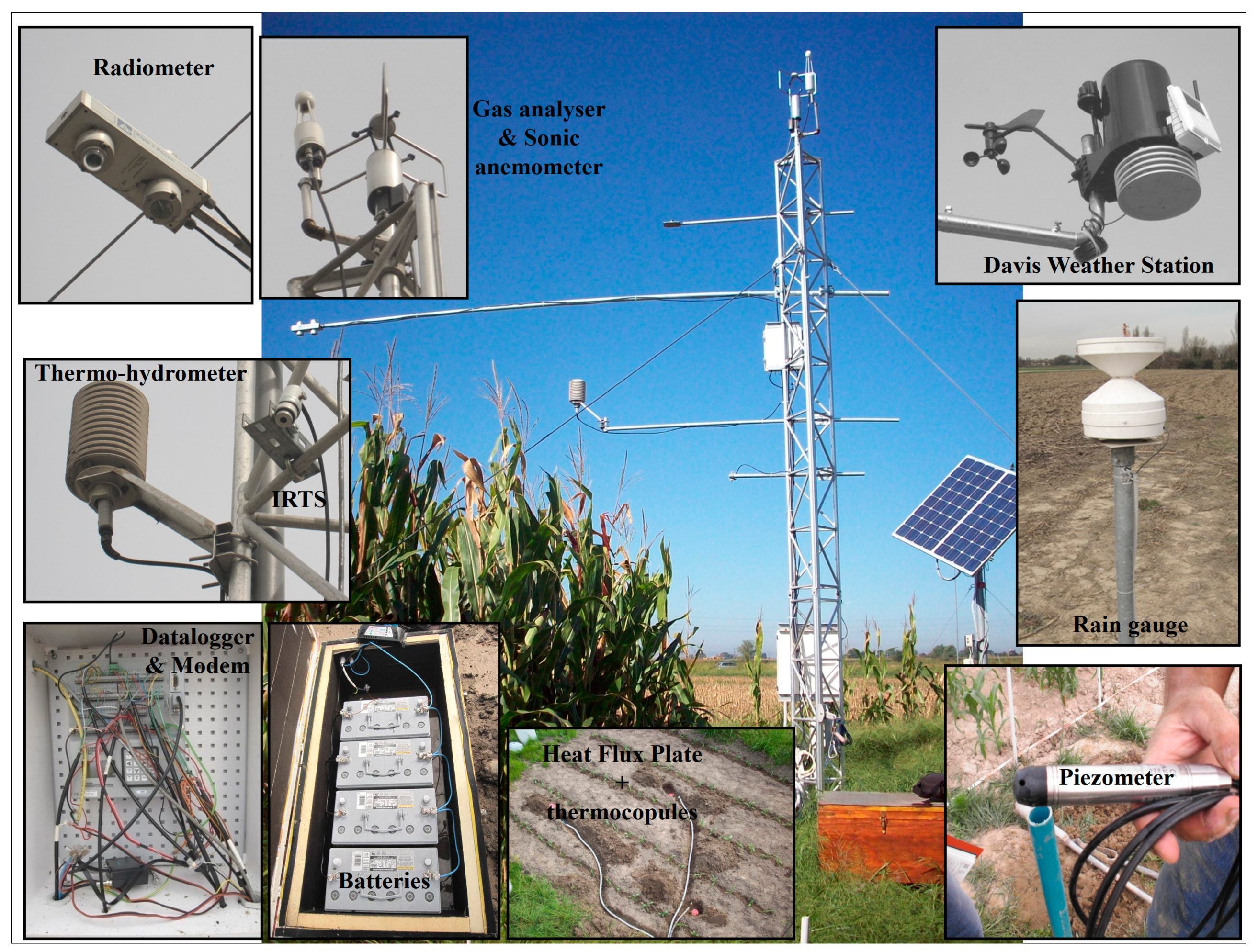
The selected experimental site for this study was an 8 ha maize field located in the middle of Muzza Bassa Lodigiana irrigation consortium in the town of Livraga in Northern Italy (45°11′26′′ N, 9°34′23′′ E) (Figure 1). Within this study site, meteorological and eddy covariance stations were installed [45,46]. The eddy covariance station is equipped with: a 3D sonic anemometer (Young 81000 by Young) placed at 5 m height together with a gas analyzer (LICOR 7500 by LICOR), two thermocouples (by ELSI), a heat flux plate (HFP01 by Hukseflux), a net radiometer (CNR1 by Kipp and Zonen) at 3 m height and an IRTS (by Apogee) for land surface temperature monitoring [46,47,48]. Meteorological data were collected at hourly time intervals. TDR probes (CS 616 probe by Campbell Scientific) were introduced at three depths of the soil profile: 10 cm, 30 cm and 70 cm. Soil moisture measurements in this field were monitored for both uncultivated (bare soil) and cultivated parts. For this study, only the cultivated part was considered. A weighted average of the three measurements was calculated giving the soil water content of the root zone.

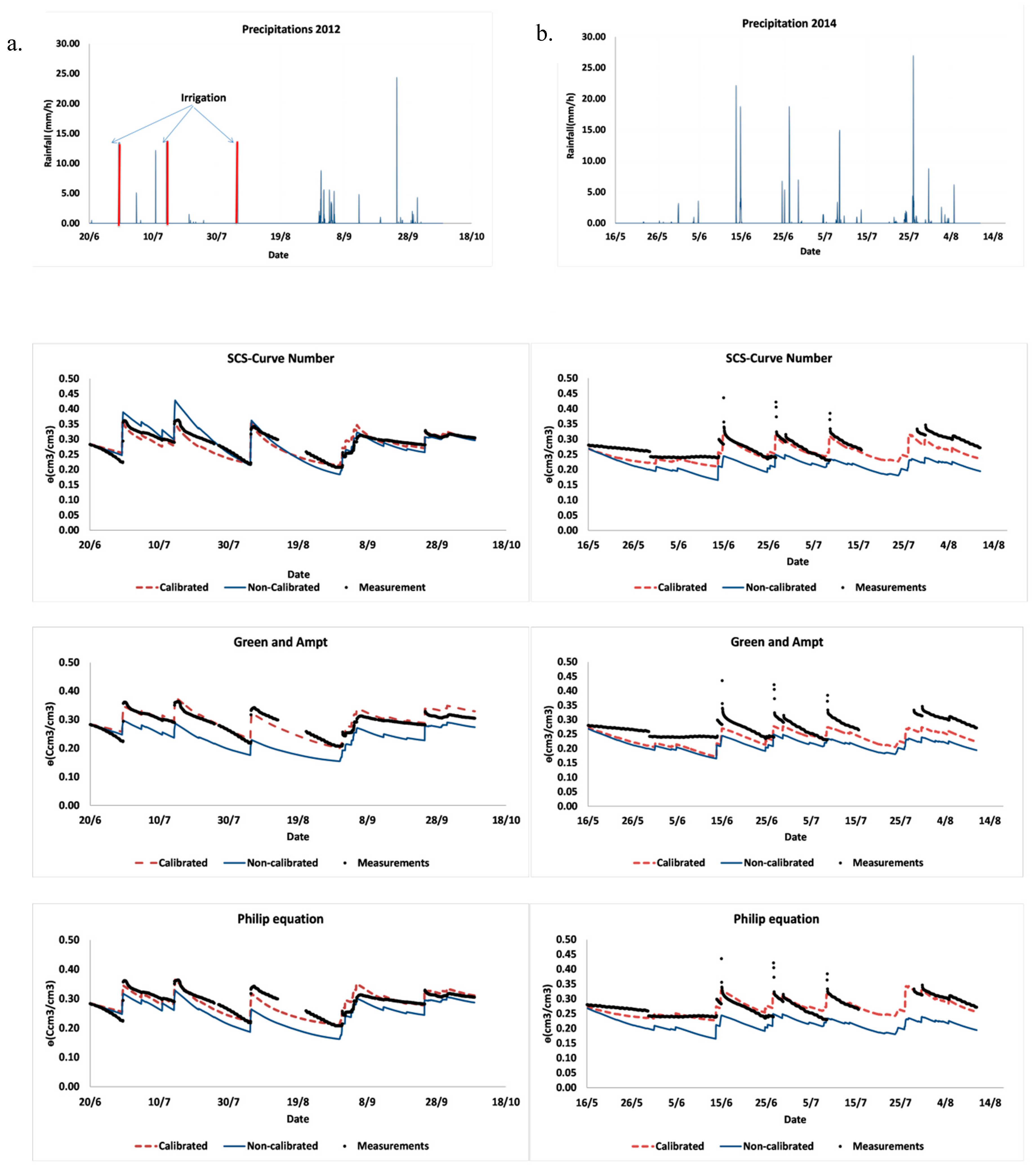
This study site, which is a surface irrigated field, was monitored for several years (2009–2014) within the framework of PREGI project (PREdiction and Guiding Irrigation) [47]. Usually, for this study area, the evapotranspiration reaches 500 mm in summer season, while the average annual precipitation varies between 800 and 1000 mm [49]. Within the cropping season of 2012, the field was irrigated three times on 29 June and 14 July and 6 August 2012. During 2014 cropping season, the field did not receive any irrigation since it was considered a rainy year and no water stress conditions were observed. During each irrigation event, about 108 mm of water were applied within 8 h.

Particle size distribution of the soil was determined in the laboratory. The soil of the study area was classified according to the USDA (United States Department of Agriculture) system of soil classification. Soil hydraulic properties presented in the

Table 1. Soil properties of Livraga study site.

Parameter	Value
Water content at Saturation (m3/m3)	0.501
Residual water content (m3/m3)	0.015
Water content at field capacity (m3/m3)	0.33
Water content at wilting point (m3/m3)	0.133
Saturated hydraulic conductivity (m/s)	2.36 E−7
% Sand	32.73
% Silt	48.08
% Clay	19.19
Soil texture	Loamy

were determined in the laboratory.

To assess the irrigation schedule implemented within the study area, we tried to control the occurrence of stress and surplus conditions. The evaluation of the stress and surplus conditions was carried out according to a fixed stress and surplus thresholds. The stress threshold was calculated according to the following equation:

$$\mathrm{Stress}\mathrm{Threshold}={\theta }_{FC}-p\times ({\theta }_{FC}-{\theta }_{WP})$$

(23)

where θ_FC the water is content at field capacity [L³/L³] and θ_WP is the water content at the wilting point [L³/L³]. p is the allowable depletion that depends on the crop was assumed equal to 0.5 for maize crop [50]. The water surplus takes place when the value of the soil moisture exceeds the θ_FC.

2.3. Model Simulations

The FEST-WB distributed hydrological model [47,49] was used for the simulation of soil moisture dynamics. Different infiltration models were implemented within FEST-WB. The initial soil moisture conditions were fixed according to the field measurements. Simulations were carried out for a homogeneous soil profile with 50 cm depth where the plants roots were mostly concentrated. Soil water content data from the study site were used to calibrate the model for the cropping season of 2012, while 2014 data were used to validate it. Bottom boundary conditions were set to free drainage conditions. The water flow in the vadose zone was not affected by the water table located at more than 2 m depth below soil surface. Upper boundary condition was controlled by atmospheric conditions (evapotranspiration and precipitation).

The potential evapotranspiration was computed according to Hargreaves–Samani model [51]:

$$T0=0.0023\times \left(KT\right)\times \left(Tav+17.8\right)\times {\left(Tmax-Tmin\right)}^{0.5}\times Ra$$

(24)

where ET0 is the reference evapotranspiration [mm/day], Ra is the extraterrestrial radiation [mm/day], KT is an empirical coefficient, and Tav, Tmax and Tmin are the average, maximum and minimum temperatures (°C), respectively. Subsequently, the crop evapotranspiration was calculated as an adjustment of the ET0 according to the crop coefficient (Kc) (

Table 2. Crop coefficient of maize.

Crop	Kcini	Kcmid	Kcend
Maize	0.26	1.02	0.62

). The Kc and the duration of development stages of the maize crop were determined according to the FAO 56, [50].

$$ET=ET0\times Kc$$

(25)

where ET is the crop evapotranspiration [L/T] and Kc is the crop coefficient.

At each time step, the ET was adjusted to the actual evapotranspiration depending on the value of the soil water content:

$$ETa=\frac{ET\times \left({\theta }_i-{\theta }_{wp}\right)}{\left({\theta }_{FC}-{\theta }_{wp}\right)}$$

(26)

where ETa is the actual evapotranspiration [L/T], θ_i is the water content at time t [L³/L³], θ_FC is the water content at the field capacity [L³/L³] and θ_wp is the water content at the wilting point [L³/L³].

At each time step, the soil water content is calculated according to the following formula:

$${\theta }_{t+1}={\theta }_t+\left(\left(\frac{I-D-ET}{Z}\right).\mathsf{\Delta }t\right)$$

(27)

where θ_t+1 is the water content at the time t + 1 [L³/L³], θ_t is the water content at time t [L³/L³], I is the infiltration rate [L/T], D is the drainage rate [L/T], ET is the actual evapotranspiration [L/T], Z is the soil depth [L] and Δt is the time step [T].

The drainage for the SCS-CN, Green and Ampt, and Philip models is calculated based on:

$$D=Ks{\left(\frac{{\theta }_t-{\theta }_r}{{\theta }_S-{\theta }_r}\right)}^{\left(\frac{2-3\lambda }{\lambda }\right)}$$

(28)

where Ks is the saturated hydraulic conductivity [L/T], θ_t is the water content at time t [L³/L³], θ_r is the residual water content [L³/L³], θ_s is the water content at saturation [L³/L³], and λ is the Brooks and Corey parameter.

For this study, the evaluation of simulations accuracy was limited to soil water content output for the tested models since that was the only available field measured data. For this aim, we selected two indicators: R² and RMSE.

• Coefficient of determination R²:

R² corresponds to the coefficient of correlation according to Bravais–Pearson.

$$R^2={\left(\frac{{{\displaystyle \sum }}_{i=1}^n\left(O_i-\overline{O}\right)\left(P_i-\overline{P}\right)}{\sqrt{{{\displaystyle \sum }}_{i=1}^n{\left(O_i-\overline{O}\right)}^2}\sqrt{{{\displaystyle \sum }}_{i=1}^n{\left(P_i-\overline{P}\right)}^2}}\right)}^2$$

(29)

where O is the field measured soil moisture and P is the estimated soil moisture. The range of variation of this coefficient is between 0 and 1, where 0 means that no correlations exist between simulations and measurements while 1 means that the dispersion of the simulations is equal to the observations [27].

• Root mean square error RMSE

$$\mathrm{RMSE}={\left[\frac{1}{n}{\displaystyle \sum }_{i=1}^n{\left(O_i-P_i\right)}^2\right]}^{1/2}$$

(30)

With n is the number of observations, O is the field measured soil moisture and P is the estimated soil moisture.

2.4. Sensitivity Analysis

Model outputs depend not only on the model structure but also on the implemented input parameters. The sensitivity analysis measures the effect of changes of input parameters on the model outputs. This step allows detecting the importance of each input parameter on the model outputs that should be considered during the calibration and validation [52]. For this study, we carried out local sensitivity analysis of the soil related parameters for each infiltration model, following one-at-a-time approach (OAT). The procedure was carried out by varying a given parameter individually by a given percentage. A Δx value of 20% was fixed regardless the potential range of variation of the tested parameters. This method is considered the easiest way to carry out sensitivity analysis and is frequently used in the literature [53]. In addition, it allows detecting the effect of each single parameter. The sensitivity of model outputs to the changes of the input parameters is expressed by a dimensionless sensitivity index. The base value is changed by $\pm \mathsf{\Delta }x$ with $x_1=x_0-\mathsf{\Delta }x$ and $x_2=x_0+\mathsf{\Delta }x.$ The model output resulting from the implementation of these values are $y_1$ and $y_2$. The sensitivity index is computed as follows:

$$I^{\prime }=\frac{y_2-y_1}{2\mathsf{\Delta }x}$$

(31)

This index $I^{\prime }$ should be normalized to be dimensionless

$$I=\frac{\left(y_2-y_1\right)/y_0}{2\mathsf{\Delta }x/x_0}$$

(32)

A positive value of this index means that, the increase of the input parameter yields an increase of the model input. Instead, a negative value implies that the increase of input yields a decrease of the output. The sensitivity index was averaged for the whole simulation period and the sensitivity of the model output to each tested input parameter was ranked according to

Table 3. Sensitivity index classes.

Class	Index	Sensitivity
Ι	$0.00\le \left|{\rm I}\right|<0.05$	Small to negligible
ΙΙ	$0.05\le \left|{\rm I}\right|<0.2$	Medium
ΙΙΙ	$0.2\le \left|{\rm I}\right|<1.00$	High
ΙV	$\left|{\rm I}\right|\ge 1.00$	Very high

as suggested by [54].

3. Results and Discussions

3.1. Results of the Sensitivity Analysis

Initial values were chosen based on measured or estimated parameters previously implemented for this study site by [47]. Sensitivity analysis was carried out by varying one parameter at a time while other parameters were set to their base values.

As presented in

Table 4. Sensitivity of SCS-CN Philip and Green and Ampt models’ output to soil hydraulic input parameters.

	Soil Moisture	Infiltration	Drainage	Evaporation
SCS-CN
Saturated hydraulic conductivity	III	II	III	II
Saturated water content	IV	II	IV	IV
Residual water content	I	I	I	I
Field capacity	III	II	IV	IV
Wilting point	I	I	II	II
Pore size distribution index	III	II	IV	II
Curve number	IV	IV	IV	II
Philip equation
Saturated hydraulic conductivity	II	III	IV	I
Saturated water content	IV	III	IV	IV
Residual water content	I	I	II	I
Alpha	II	III	IV	I
Field capacity	III	II	IV	IV
Wilting point	I	I	III	II
Pore size distribution index	III	II	IV	III
Green and Ampt
Saturated hydraulic conductivity	II	III	IV	II
Saturated water content	IV	III	IV	IV
Residual water content	II	I	III	I
Alpha	I	I	I	I
Field capacity	II	II	IV	IV
Wilting point	I	I	III	II
Pore size distribution index	III	II	IV	III
Suction	II	III	IV	II

, almost the same sensitivity to the tested soil hydraulic parameters was recorded for all tested outputs: infiltration, soil moisture, evapotranspiration and drainage to account for the interdependency of these processes. The residual and wilting point water content had almost no effect or negligible influence on the simulation results for all tested models. For SCS-CN, high sensitivity was recorded for the saturated water content and CN parameters.

Philip and GA models were more sensitive to saturated water content, saturated hydraulic conductivity and pore size distribution index. Similarly, the suction head at the wetting front of GA had an important impact on all model outputs.

Sensitivity analysis was conducted for both Ross-BC and Ross-VG (

Table 5. Sensitivity of Ross model output to soil hydraulic input parameters.

	Soil Moisture	Infiltration	Drainage	Evaporation
Ross-BC
Saturated hydraulic conductivity	III	II	II	II
Saturated water content	IV	II	IV	III
Residual water content	I	I	I	I
Alpha	I	I	III	III
Field capacity	II	I	III	III
Wilting point	I	I	I	I
Pore size distribution index	III	II	III	II
Ross-VG
Saturated hydraulic conductivity	III	II	III	III
Saturated water content	IV	II	IV	IV
Residual water content	I	I	I	I
Alpha	III	I	III	III
Field capacity	II	I	III	IV
Wilting point	I	I	I	I
n	III	II	II	III
m	IV	II	III	III

). The evaluation of sensitivity was carried out for the average water content within the 50 cm soil profile as well to the other model outputs. For soil moisture simulations, the model was sensitive to the saturated hydraulic conductivity and saturated water content compatibly to what was found for the other implemented infiltration models. For Ross-BC, pore size distribution was the most sensitive parameter. Similarly, for Ross-VG, n and m were sensitive parameters. This step allowed us to detect the parameters that affect more the simulation results, in particular for soil moisture.

3.2. Results of the Sensitivity Analysis

The next step was to calibrate the model. The calibration objective was to select the model parameters that allow best soil moisture simulations as compared to field measurements for the cropping year of 2012. Insensitive parameters, such as residual water content, were fixed to their initial values. The main optimized parameters during this calibration were the saturated hydraulic conductivity and saturated water content. Even if they are based on different assumptions, the implemented Green and Ampt, SCS-CN and Philip’s models within the FEST-WB allowed reaching good performances.

Table 6. Comparison between the performances of the simulation of soil moisture based on different implemented infiltration models before and after calibration for 2012 and 2014 cropping seasons.

Calibration Year 2012	RMSE (cm3/cm3)				Validation Year 2014	RMSE (cm3/cm3)
	Philip	Green and Ampt	SCS-CN	Multimodel		Philip	Green and Ampt	SCS-CN	Multimodel
Before calibration	0.041	0.059	0.023	0.037	Before calibration	0.046	0.06	0.039	0.047
After calibration	0.019	0.02	0.019	0.02	After calibration	0.017	0.039	0.025	0.024
Calibration Year 2012	R2				Validation Year 2014	R2
	Philip	Green and Ampt	SCS-CN	Multimodel		Philip	Green and Ampt	SCS-CN	Multimodel
After calibration	0.74	0.83	0.74	0.80		0.66	0.57	0.61	0.65

presents the RMSE and R² for the both calibration and validation years. The calculated performance indicators RMSE and R² confirm the improvement of the simulation after the calibration. Even before calibration, good performances were reached in particular for SCS-CN with RMSE equal to 0.023. After calibration, similar RMSE values were found of about 0.019, 0.020 and 0.019 for SCS-CN, Green and Ampt and Philip models respectively.

The set of soil hydraulic parameters found during the calibration period, were used to validate the model. The validation was carried out for the 2014 year. The results during the calibration period were slightly better than for the validation. As presented in Table 6, there was no significant degradation of the results between the calibration and the validation of all models. The R² proved this result with 0.74, 0.83, and 0.74 for the calibration year and 0.66, 0.57, and 0.61 for the validation year for Philip, GA and SCS-CN, respectively, consequently with slight advantage to Philip model with RMSE of 0.017 after the calibration.

Figure 2 shows the results in reproducing the soil moisture variation during the cropping season of 2012 and 2014. This figure shows satisfactory results of different simulations to detect the variability of soil moisture. Better performances were observed in particular during the irrigation period of the year 2012. Through these simulations for this study site, it was not possible to rank the infiltration models based on their accuracy to simulate the soil moisture variation since similar performances were achieved. For an application for irrigation management, all models showed good performances in terms of detecting the critical soil water contents when the irrigation should be applied.

Introduced within the same model and by carrying out the simulations under the same boundary condition, the only difference between all these simulations is the model used for the calculation of infiltration. From the results presented in Table 6 and Figure 2, it has been proven that when SCS-CN, GA or Philip equations were implemented differences in soil moisture simulations were negligible. The introduced calibrated input parameters required for different infiltration model simulations under the same climatic forcing were different. This finding is due to the difference of the model structures.

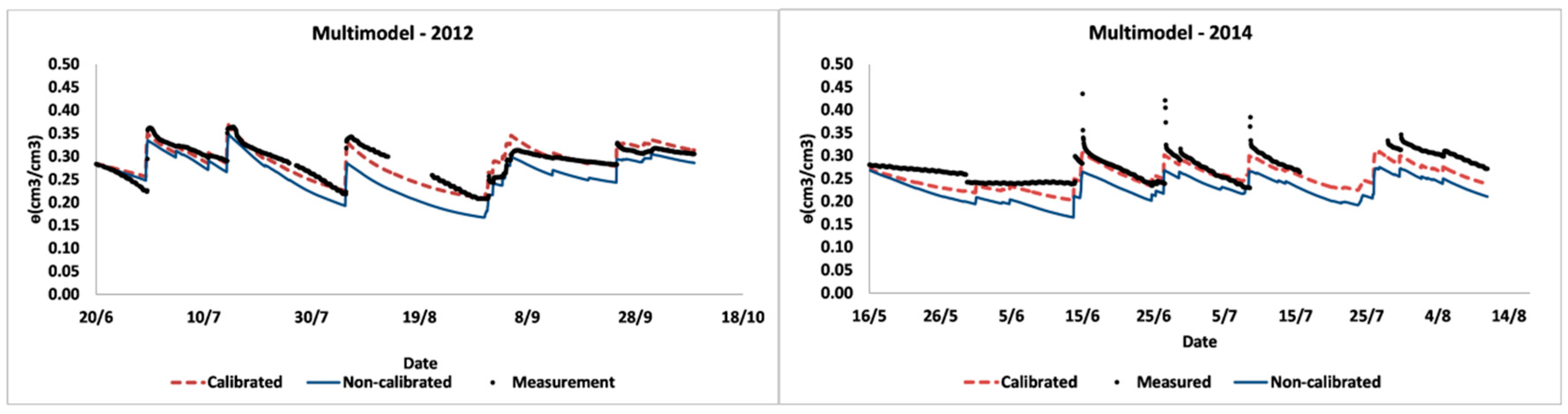
To overcome limitations and uncertainties induced from a model structure, a multiple-model simulation has been suggested by many researchers [55]. To reduce the uncertainty induced from the implementation of a single analytical solution that is based on different assumptions, a multimodel average was applied. The implementation of different models for the calculation of the infiltration into the FEST-WB model allowed us to implement this modeling approach. A simple Multi-Model Ensemble Approach based on arithmetic averaging of the results of simulation of SCS-CN, Green and Ampt and Philip model results was adopted. This method has been considered as quite effective [56]. Usually, this approach is used to combine the outputs of different hydrological model simulations. For this study, the same FEST-WB model was used but with different implemented models to solve the infiltration process. As presented in Figure 3 and Table 6, this multimodel average gave good estimates of the soil moisture variability even without calibration. It should be noted that some of the implemented parameters within these infiltration models were taken from the literature while others were measured in laboratory with a physical meaning. Under these conditions, applying this approach even without calibration allowed reaching good performances. Implemented for the validation year, multimodel averaging gave a RMSE of 0.024 while the RMSE for CN, GA and Philip models was equal to 0.017, 0.039 and 0.025, respectively.

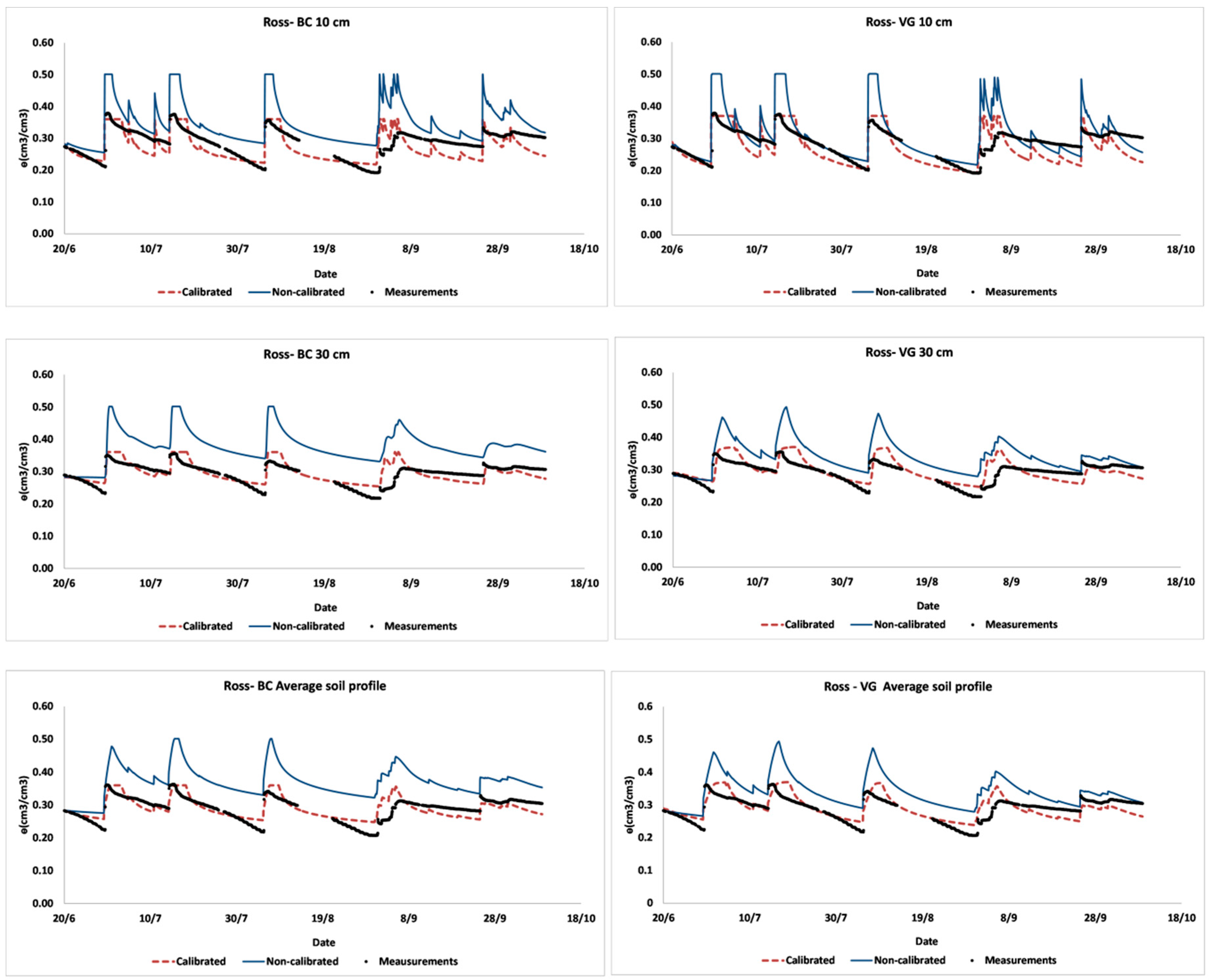
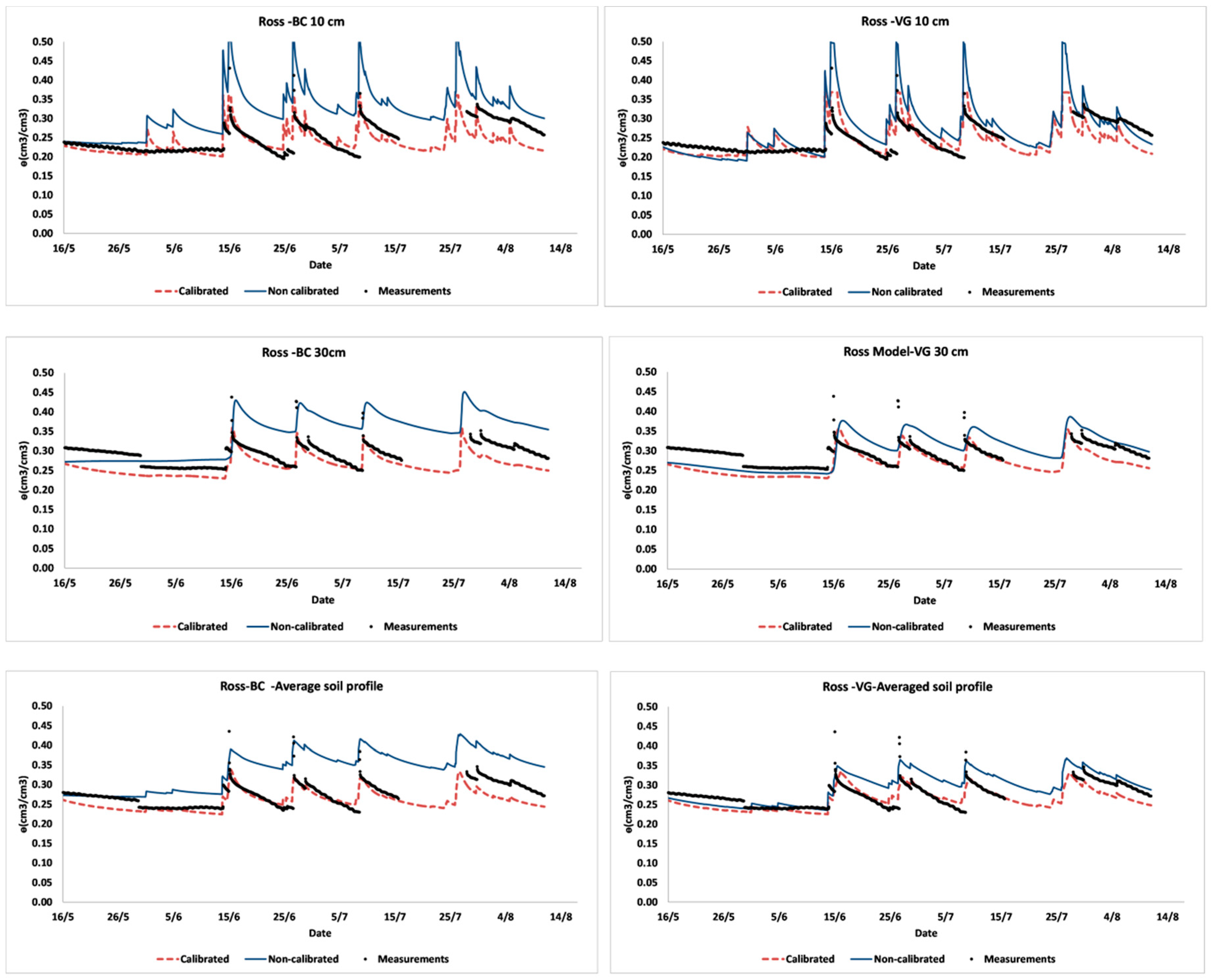
The implementation of Ross model gave us the possibility to assess the performances of the simulations of the soil moisture at the two observation points 10 cm and 30 cm (Figure 4 and Figure 5). The performances of Ross model were assessed at these two depths as well for the average soil profile (

Table 7. Performances of the simulation of soil moisture based on Ross Model based on Brooks and Corey and Van Genuchten parametric equations before and after calibration for 2012 and 2014 cropping seasons.

Calibration Year 2012	RMSE						Validation Year 2014	RMSE
	Ross-BC			Ross-VG				Ross-BC			Ross-VG
Depth	10 cm	30 cm	Average	10 cm	30 cm	Average	Depth	10 cm	30 cm	Average	10 cm	30 cm	Average
Before calibration	0.077	0.094	0.089	0.062	0.069	0.062	Before calibration	0.081	0.066	0.07	0.051	0.036	0.034
After calibration	0.035	0.024	0.276	0.041	0.028	0.026	After calibration	0.032	0.032	0.023	0.034	0.031	0.021
Calibration Year 2012	R2						Validation Year 2014	R2
	Ross-BC			Ross-VG				Ross-BC			Ross-VG
Depth	10 cm	30 cm	Average	10 cm	30 cm	Average	Depth	10 cm	30 cm	Average	10 cm	30 cm	Average
After calibration	0.49	0.48	0.56	0.53	0.50	0.54		0.28	0.56	0.55	0.33	0.46	0.57

). Although based on different parametric equations for soil water retention and conductivity curves, similar performances were achieved for both Ross-VG and Ross-BC with RMSE of 0.0276 and 0.0263 for the calibration year and RMSE of 0.0231 and 0.0211 for the validation year, respectively. The lowest performances were attributed to the first 10 cm of the soil profile. At this depth, for the calibration year the RMSE and R² for Ross-BC were 0.035 and 0.49 while for the validation year were 0.032 and 0.28, respectively. For Ross-VG, these values were 0.041 and 0.53 for the calibration year and 0.034 and 0.33 for the validation year, respectively. The top soil was subjected to high fluctuations of soil moisture, which caused more soil moisture variability that was observed in the measured water content at 10 cm soil depth. This is also because the top soil is more subjected to the evaporative fluxes as well as to the disturbance of the soil structure during the cropping season. One set of parameters was considered for whole soil profile that is supposed to be homogeneous. Capturing these fluctuations was not possible when the average soil moisture of the 50 cm soil profile was considered.

Ross model has more input parameters than other analytical models to be calibrated adding more uncertainty in the overall soil moisture simulation results. Similar to all physically based models, the Ross solution is more sensitive to the implemented input parameters than empirical models, hence the calibration for Ross solution was more complicated. As compared to other numerical schemes, the non-iterative Ross solution was faster at solving the Richards equation.

3.3. Evaluation of Irrigation Scheduling

Proper irrigation management requires that growers’ decision should be taken based on some indicators based on monitoring of soil water status. Irrigation scheduling aims at determining how much water to apply and when to irrigate [57]. The proper amount of irrigation and timing are based on several factors: soil and plant characteristics and climatic conditions. Irrigation scheduling based on soil moisture has been widely implemented. A combined use of monitoring and modeling allowed the use of such simulations coupled with meteorological forecasts for irrigation management purposes [47]. Model simulations have been used also to identify the influencing factors on the cumulative infiltration of a given irrigation technique [58]. Hence, the model accuracy is very important when implemented for this aim. Right decisions are taken based on right data while uncertain model simulations lead to unreliable results and thus inadequate decisions.

In this study, we evaluated the effect of the infiltration model into the FEST-WB model by assessing the efficiency of irrigation water application during 2012 cropping cycle. As the study area is located within a rotational irrigation delivery scheme, the water allocation at each farm is possible every 14 days. The water is then distributed at a fixed rotation with the same volume per farm. Water is delivered to farms through collective irrigation canal. Irrigation turns, discharge and duration are fixed by the consortium. In such case, due to the non-flexibility of the delivery systems, farmers irrigate whenever the water is available. In such circumstances, farms are over irrigated [59]. Both farmers and irrigation scheme managers should be aware of the negative impacts of such practices (lack of oxygen for plants, leachate of fertilizers, water losses, etc.).

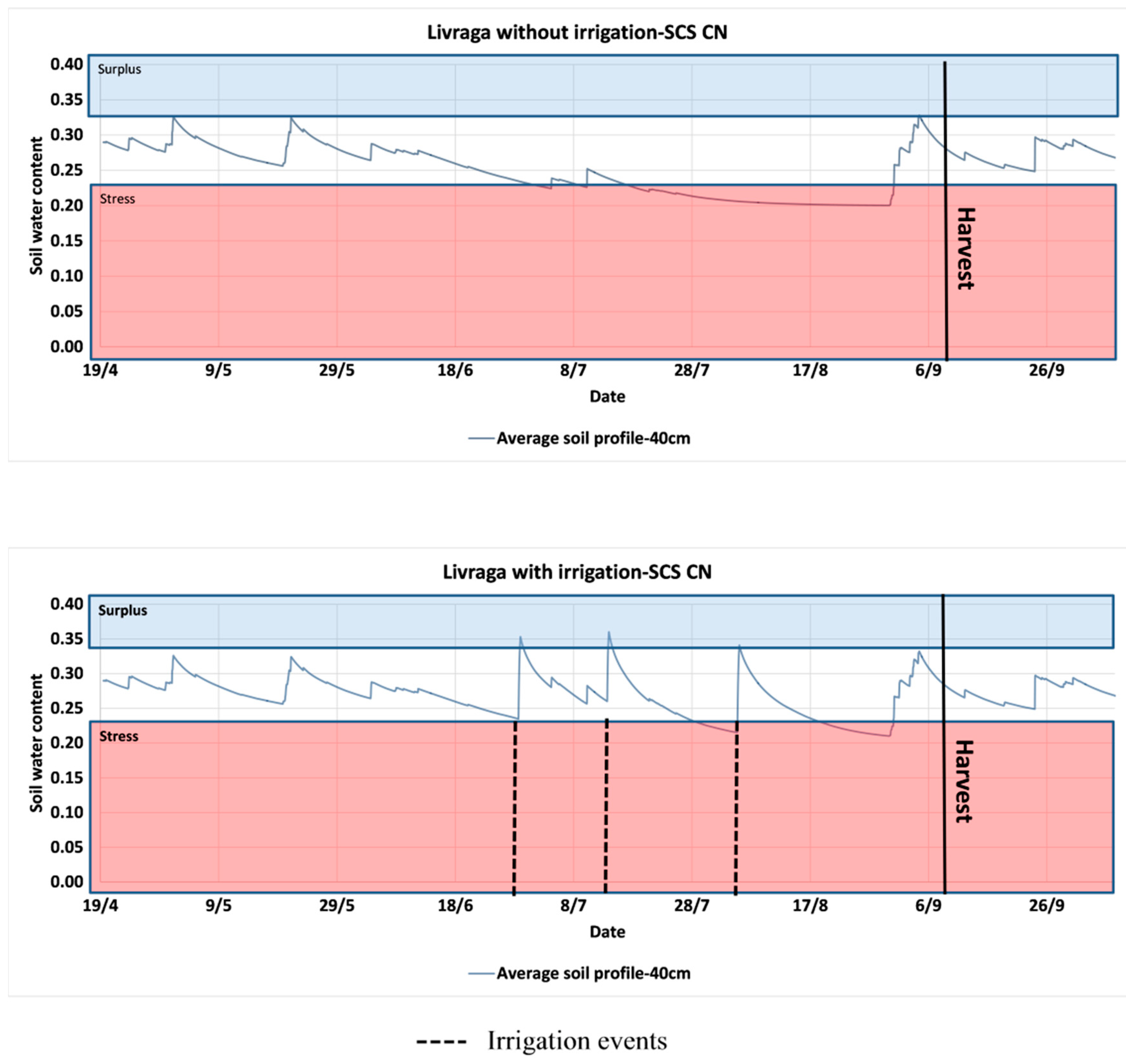
The most critical concern for irrigation scheduling, is the timing at which the water content reaches stress threshold, which in this study is equal to 0.23 cm³/cm³. The uncertainty of the model, implemented as decision support tool to plan irrigation water applications, is critical. About this issue, we selected SCS-CN and Ross-VG to carry out our analyses. Figure 6 and Figure 7 present the results of simulations based on Ross-VG and SCS-CN respectively. Simulations without irrigation showed that more stress conditions appeared in particular during summer season when the crop was fully developed. The occurrence of surplus conditions could not be avoided and occurred after a heavy rainfall or irrigation. Simulations based on SCS-CN did not allow assessing the water stress presence at different soil depths. The irrigation should be applied when the stress threshold is reached. In terms of evaluation of effectiveness of the irrigation based on the Figure 6, it can be concluded that at irrigation was applied at a good timing when the soil water content reached the stress threshold. This irrigation allowed avoiding stress conditions that were observed for the no-irrigation scenario.

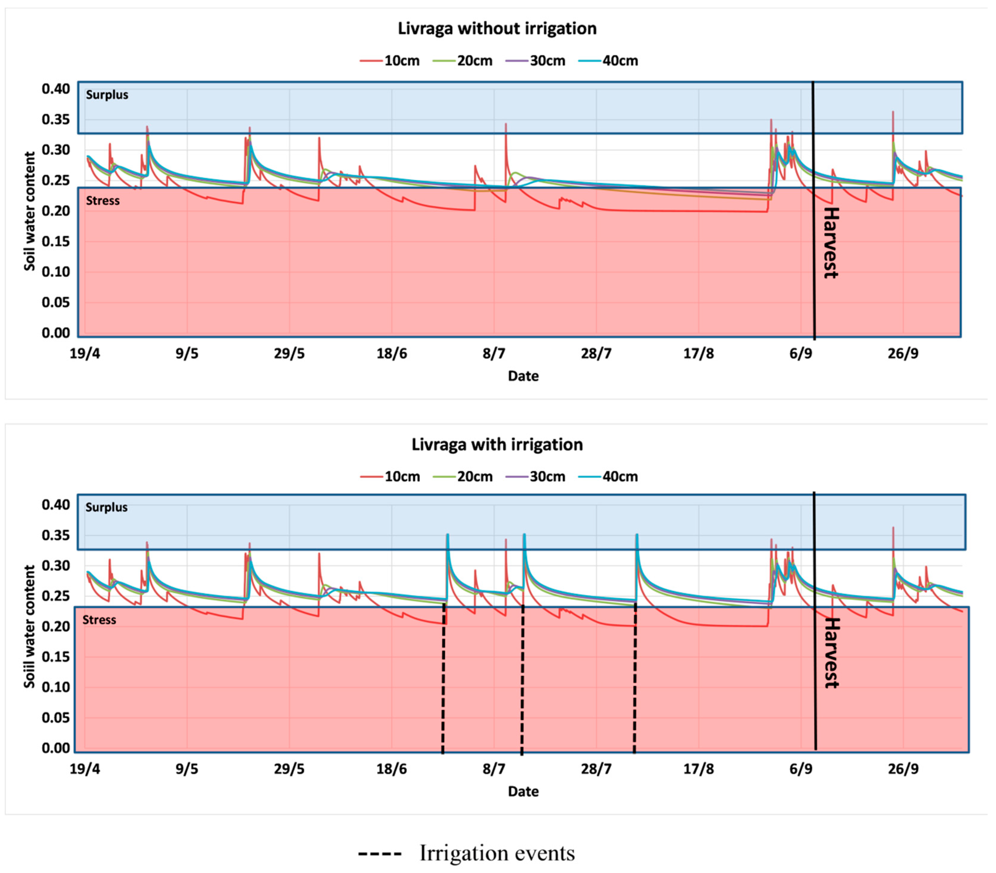
The lack of information about water content variation at different soil depths can mislead the results of assessment of stress occurrence in time as well as the irrigation scheduling itself. The use of Ross solution, allowed overcoming this limitation. As presented in Figure 7, it was possible to observe that water depletion was different from one soil layer to another during the cropping season. In contrast to the conclusions drawn from Figure 6, irrigation did not allow completely avoiding stress conditions mainly for the first 10 cm of the soil profile. It is obvious that, under surface irrigation conditions, where the irrigation is not frequent, it was not possible to avoid the stress conditions in the first 10 cm where the water was quickly depleted due to evaporative fluxes. Stress was not limited to the 10 cm soil depth but reached even deeper soil. At 20 cm soil depth, less stress was observed for simulations where irrigation was applied. For the 30 cm layer, even without irrigation we observed only short period of stress.

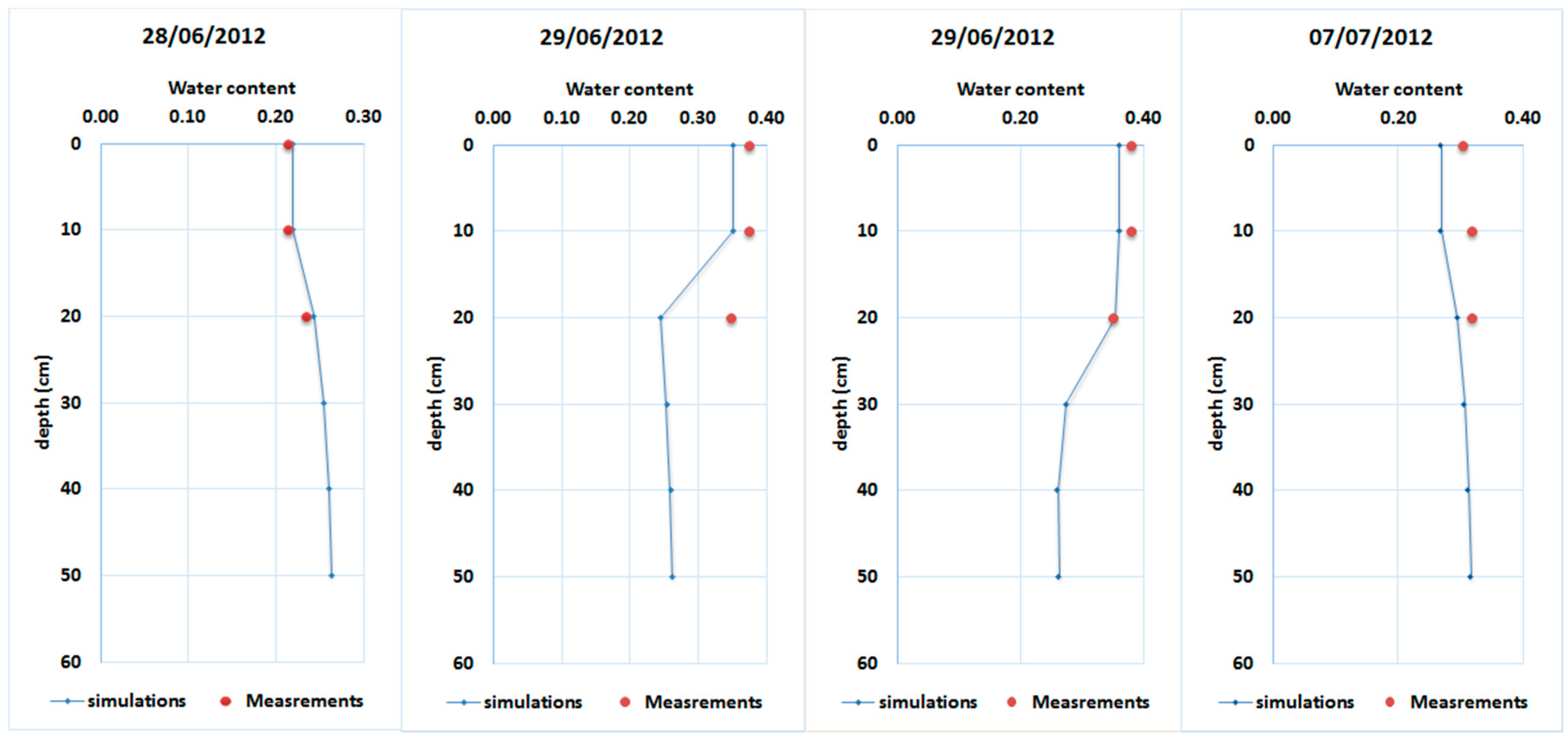
Figure 8 shows the variability of soil moisture within the soil profile before, during and after an irrigation event as simulated based on Ross model. This figure allows following the variability of the soil water content before, during and after an irrigation event within the soil profile.

As presented in Figure 8, the simulations reproduced quite well the measured values at different depths. The first presented soil profile on 28 June corresponds to dry conditions while the second and third profiles corresponds to wet conditions under irrigation on 29 June. These profiles show the ability of the FEST-WB when Ross solution is implemented to capture the variability of soil moisture under dry and wet conditions when compared to field measurements. During the irrigation event (the first profile of 29 June), an increase of the soil moisture was observed within the first 10 cm at a first step, then few hours later (the second profile of the 29 June), the wetting front moved downward to deeper soil. Few days after the irrigation event on 7 July, a depletion of the water content was observed in particular at the surface. This information is very important if the model will be used as decision support for irrigation management in particular for localized irrigation systems.

4. Conclusions

This study dealt with parameter sensitivity and performances of different implemented infiltration models within the FEST-WB model. The simulations were carried out under similar modeling conditions: rainfall, soil, vegetation, etc. The differences in the soil moisture simulations were only due to difference of the models used for the infiltration calculations. The accuracy of soil moisture simulations based on different infiltration models has been evaluated against field measurements. The accuracy of numerical solutions of Richards’ equation, as well as analytical solutions, highly depends on the quality of input data, which are the hydraulic conductivity and water retention curve parameters. Tested analytical solutions gave good performances as compared to field measured soil moisture; a good calibration has great importance for improving these performances. Implementing different equations for infiltration simulation within the same model allowed the implementation of a multimodel ensemble approach based on simple averaging of outputs of different simulations based on different infiltration models. This approach allowed reducing simulation uncertainty even without calibration.

Ross solution gave different performances for soil moisture at the monitored points of 10 cm and 30 cm, which highly depends on the quality of input parameters. Lower accuracy was achieved for the top soil layer that is more subjected to fluctuations of water contents and to disturbance during the cropping season. Knowing the water content at different depths of the soil profile is crucial when implemented for irrigation management. Ross solution gave the possibility to follow the soil moisture variability within the soil profile, which is highly recommended in particular for the case of localized irrigation practices. For this study site, good overall agreement between field measured and simulated soil moisture was achieved when analytical infiltration models or physically based Ross solution were used.

Determining the irrigation timing and the amount of water to satisfy the plants requirements is very complicated. About on demand irrigation schemes, deciding when to start the irrigation has always been a challenging task. It can be concluded from performed analysis that decision of the farmer cannot always guarantee reaching optimal and efficient irrigation scheduling. A decision support tool for better management of water resources is highly recommended. Results of this study proved that the selection of the infiltration model for the simulation of the soil water movement and assessment of the occurrence of water stress conditions produced different results and different conclusions. The selection of the model to be used for such purposes should consider the degree of precision and the information required for a better management of irrigation water.

Further studies are required to assess the accuracy of different tested infiltration models under different field conditions. The limitation of the one at a time sensitivity analysis is that the interactions between the parameters cannot be considered. As a further step, global sensitivity can be implemented for a better understanding of these interactions.

References

- Haghiabi, A.H.; Heidarpourand, M.; Habili, J. A new method for estimating the parameters of Kostiakov and modified Kostiakov infiltration equations. World Appl. Sci. J. 2011, 15, 129–135. [Google Scholar]
- Zolfaghari, A.A.; Mirzaee, S.; Gorji, M. Comparison of different models for estimating cumulative infiltration. Int. J. Soil Sci. 2012, 7, 108–115. [Google Scholar] [CrossRef]
- Bouma, J. Influence of soil macroporosity on environmental quality. Adv. Agron. 1991, 46, 1–37. [Google Scholar] [CrossRef]
- Merdun, H. Effects of Different Factors on Water Flow and Solute Transport Investigated by Time Domain Reflectometry in Sandy Clay Loam Field Soil. Water Air Soil Pollut. 2012, 223, 4905. [Google Scholar] [CrossRef] [PubMed]
- Mishra, S.K.; Singh, V.P. Long-term hydrological simulation based on the soil conservation service curve number. Hydrol. Processes 2004, 18, 1291–1313. [Google Scholar] [CrossRef]
- Richards, L.A. Capillary conduction of liquids in porous mediums. Physics 1931, 1, 318–333. [Google Scholar] [CrossRef]
- Lassabatere, L.; Angulo-Jaramillo, R.; Soria-Ugalde, J.M.; Simunek, J.; Haverkamp, R. Numerical evaluation of a set of analytical infiltration equations. Water Resour. Res. 2009, 45. [Google Scholar] [CrossRef] [Green Version]
- Tinet, A.-J.; Chanzy, A.; Braud, I.; Crevoisier, D.; Lafolie, F. Development and evaluation of an efficient soil-atmosphere model (FHAVeT) based on the Ross fast solution of the Richards equation for bare soil conditions. Hydrol. Earth Syst. Sci. 2015, 19, 969–980. [Google Scholar] [CrossRef] [Green Version]
- Feddes, R.A.; Kabat, P.; Van Bakel, P.J.T.; Bronswijk, J.J.B.; Halbertsma, J. Modeling soil water dynamics in the saturated zone—State of the art. J. Hydrol. 1988, 100, 69–111. [Google Scholar] [CrossRef]
- Ross, P.J. Modeling soil water and solute transport—Fast simplified numerical solutions. Agron. J. 2003, 95, 1352–1361. [Google Scholar] [CrossRef]
- Ravi, V.; Williams, J.R. Estimation of Infiltration Rate in the Vadose Zone: Compilation of Simple Mathematical Models; US Environmental Protection Agency: Washington, DC, USA, 1998; Volume I, 26p.
- Mishra, S.K.; Tyagi, J.V.; Singh, V.P. Comparison of infiltration models. Hydrol. Processes 2003, 17, 2629–2652. [Google Scholar] [CrossRef]
- Kostiakov, A.N. On the dynamics of the coefficient of water-percolation in soils and on the necessity for studying it from a dynamic point of view for purposes of amelioration. In Proceedings of the 6th Transactions Congress International Society for Soil Science, Moscow, Russia, 1932. [Google Scholar]
- Soil Conservation Service (SCS). Hydrology, National Engineering Handbook; Soil Conservation Service: Washington, DC, USA, 1985.
- Huggins, L.F.; Monke, E.I. The Mathematical Simulation of the Hydrology of Small Watersheds; Technical Report No. 1; Purdue Water Resources Centre: West Lafayette, Indiana, 1966. [Google Scholar]
- Collis-George, N. Infiltration equations for simple soil systems. Water Resour. Res. 1977, 13, 395–403. [Google Scholar] [CrossRef]
- Beasley, D.B.; Huggins, L.F.; Monke, E.J. ANSWERS: A model for watershed planning. Trans. ASAE 1980, 23, 938–944. [Google Scholar] [CrossRef]
- Sharpley, A.N.; Williams, J.R. EPIC—Erosion/Productivity Impact Calculator. I. Model Documentation; US Department of Agriculture Technical Bulletin; US Department of Agriculture: Washington, DC, USA, 1990.
- Arnold, J.G.; Moriasi, D.N.; Gassman, P.; Abbaspour, K.C.; White, M.J.; Srinivasan, R.; Santhi, C.; Harmel, R.D.; van Griensven, A.; Van Liew, M.W.; et al. SWAT: Model use, calibration, and validation. Trans. ASABE 2012, 14, 533–538. [Google Scholar]
- Philip, J.R. Numerical solution of equations of the diffusion type with diffusivity concentration-dependent II. Aust. J. Phys. 1957, 10, 29–42. [Google Scholar] [CrossRef]
- Smith, R.E.; Parlange, J.Y. A parameter-efficient hydrologic infiltration model. Water Resour. Res. 1978, 14, 533–538. [Google Scholar] [CrossRef]
- Green, W.H.; Ampt, G.A. Studies on soil physics I. Flow of air and water through soils. J. Agric. Sci. 1911, 4, 1–24. [Google Scholar]
- Varado, N.; Braud, I.; Ross, P.; Haverkamp, R. Assessment of an efficient numerical solution of the the 1D Richards’ equation on bare soil. J. Hydrol. 2006, 323, 244–257. [Google Scholar] [CrossRef]
- Crevoisier, D.; Chanzy, A.; Voltz, M. Evaluation of the Ross fast solution of Richards’ equation in unfavourable conditions for standard finite element methods. Adv. Water Resour. 2009, 32, 936–947. [Google Scholar] [CrossRef]
- Chanzy, A.; Bruckler, L. Significance of soil surface moisture with respect to daily bare soil evaporation. Water Resour. Res. 1993, 29, 1113–1125. [Google Scholar] [CrossRef]
- Vereecken, H.; Schnepf, A.; Hopmans, J.W.; Javaux, M.; Or, D.; Roose, T.; Vanderborght, J.; Young, M.H.; Amelung, W.; Aitkenhead, M.; et al. Modeling Soil Processes: Review, Key Challenges, and New Perspectives. Vadose Zone J. 2016, 15, 57. [Google Scholar] [CrossRef] [Green Version]
- Krause, P.; Boyle, D.P.; Bäse, F. Comparison of different efficiency criteria for hydrological model assessment. Adv. Geosci. 2005, 5, 89–97. [Google Scholar] [CrossRef]
- Ines, A.V.M.; Droogers, P.; Makin, I.W.; Das Gupta, A. Crop Growth and Soil Water Balance Modeling to Explore Water Management Options; IWMI Working Paper 22; International Water Management Institute: Colombo, Sri Lanka, 2001. [Google Scholar]
- Brooks, R.H.; Corey, A.T. Hydraulic Properties of Porous Media; Hydrology Paper 3; Colorado State University: Fort Collins, CO, USA, 1964. [Google Scholar]
- Van Genuchten, M. A closed-form equation for predicting the hydraulic conductivity of unsaturated soils. Soil Sci. Soc. Am. J. 1980, 44, 892–898. [Google Scholar] [CrossRef]
- Soulis, K.X.; Valiantzas, J.D. SCS-CN parameter determination using rainfall-runoff data in heterogeneous watersheds—The two-CN system approach. Hydrol. Earth Syst. Sci. 2012, 16, 1001–1015. [Google Scholar] [CrossRef] [Green Version]
- Adornado, H.A.; Yoshida, M. GIS-based watershed analysis and surface run-off estimation using curve number (CN) value. J. Environ. Hydrol. 2010, 18, 1–10. [Google Scholar]
- Moretti, G.; Montanari, A. Inferring the flood frequency distribution for an ungauged basin using a spatially distributed rainfall-runoff model. Hydrol. Earth Syst. Sci. 2008, 12, 1141–1152. [Google Scholar] [CrossRef] [Green Version]
- Ravazzani, G.; Mancini, M.; Giudici, I.; Amadio, P. Effects of soil moisture parameterization on a real- time flood forecasting system based on rainfall thresholds. In Quantification and Reduction of Predictive Uncertainty for Sustainable Water Resources Management (Proceedings of Symposium HS2004 at IUGG2007, Perugia, July 2007); IAHS Press: Wallingford, UK, 2007; pp. 407–416. [Google Scholar]
- Sivapalan, M.; Beven, K.; Wood, E.F. On hydrologic similarity, 2A scaled model of storm runoff production. Water Ressour. Res. 1987, 23, 2266–2278. [Google Scholar] [CrossRef]
- Kutilek, M.; Nielsen, R. Soil Hydrology; Geoscience Publisher: Cremlingen-Destedt Catena-Verlag, Germany, 1994; Chapter 5.3.2; pp. 104–112. [Google Scholar]
- Verseghy, D.L. CLASS—A Canadian Land Surface Scheme for GCMs. I. Soil model. Int. J. Climatol. 1991, 11, 111–133. [Google Scholar] [CrossRef]
- Bicknell, B.R.; Imhoff, J.C.; Kittle, J.L., Jr.; Jobes, T.H.; Donigian, A.S. Hydrological Simulation Program—FORTRAN (HSPF); User’s Manual for Release 12; U.S. EPA National Exposure Research Laboratory: Athens, GA, USA, 2001.
- Neitsch, S.L.; Arnold, J.G.; Kiniry, J.R.; Williams, J.R.; King, K.W. Soil Water Assessment Tool Theoretical Documentation; GSWRL Report 02-01; Grassland, Soil and Water Research Laboratory: Temple, TX, USA, 2002.
- Polsinelli, J.; Kavvas, M.L. Variable Saturation Infiltration Model for Highly Vegetated Regions. Hydrol. Earth Syst. Sci. Discuss. 2016. [Google Scholar] [CrossRef]
- Hillel, D.; Gardner, W.R. Transient infiltration into crust topped profiles. J. Soil Sci. 1970, 109, 69–76. [Google Scholar] [CrossRef]
- Bouwer, H. Infiltration of water into non-uniform soil. ASCE J. Irrig. Drain. Div. 1969, 95, 451–462. [Google Scholar]
- Childs, E.C.; Bybordi, M. The vertical movement of water in stratified porous material: 1. Infiltration. Water Resour. Res. 1969, 5, 446–459. [Google Scholar] [CrossRef]
- Mein, R.G.; Larson, C.L. Modeling infiltration during a steady rain. Water Resour. Res. 1973, 9, 384–394. [Google Scholar] [CrossRef]
- Rawls, W.J.; Brakensiek, D.L.; Soni, B. Agricultural management effects on soil water processes, I, Soil water retention and Green and Ampt infiltration parameters. Trans. ASAE 1983, 26, 1747–1752. [Google Scholar] [CrossRef]
- Masseroni, D.; Corbari, C.; Mancini, M. Limitations and improvements of the energy balance closure with reference to experimental data measured over a maize field. Atmosfera 2014, 27, 335–352. [Google Scholar] [CrossRef] [Green Version]
- Ceppi, A.; Ravazzani, G.; Corbari, C.; Salerno, R.; Meucci, S.; Mancini, M. Real-time drought forecasting system for irrigation management. Hydrol. Earth Syst. Sci. J. 2014, 18, 3353–3366. [Google Scholar] [CrossRef] [Green Version]
- Corbari, C.; Mancini, M.; Li, J.; Su, Z. Can satellite land surface temperature data be used similarly to ground discharge measurements for distributed hydrological model calibration? Hydrol. Sci. J. 2015, 60, 202–217. [Google Scholar] [CrossRef]
- Ravazzani, G.; Corbari, C.; Ceppi, A.; Feki, M.; Mancini, M.; Ferrari, F.; Gianfreda, R.; Colombo, R.; Ginocchi, M.; Meucci, S.; et al. From (cyber) space to ground: New technologies for smart farming. Hydrol. Res. 2017, 48, 656–672. [Google Scholar] [CrossRef]
- Allen, R.G.; Pereira, L.S.; Raes, D.; Smith, M. Crop Evapotranspiration: Guidelines for Computing Crop Water Requirements; Irrigation and Drainage Paper No. 56; Food and Agriculture Organization of the United Nations: Rome, Italy, 1998. [Google Scholar]
- Hargreaves, G.H.; Samani, Z.A. Reference crop evapotranspiration from temperature. Trans. ASAE 1985, 1, 96–99. [Google Scholar] [CrossRef]
- Moriasi, D.N.; Arnold, J.G.; Van Liew, M.W.; Bingner, R.L.; Harmel, R.D.; Veith, T.L. Model evaluation guidelines for systematic quantification of accuracy in watershed simulations. Trans. ASABE 2007, 50, 885–900. [Google Scholar] [CrossRef]
- Hamby, D.M. A review of techniques for parameter sensitivity analysis of environmental models. Environ. Monit. Assess. 1994, 32, 135–154. [Google Scholar] [CrossRef] [PubMed] [Green Version]
- Lenhart, T.; Eckhardt, K.; Fohrer, N.; Frede, H.-G. Comparison of two different approaches of sensitivity analysis. Phys. Chem. Earth 2002, 27, 645–654. [Google Scholar] [CrossRef]
- Kim, J.; Mohanty, B.P.; Shin, Y. Effective soil moisture estimate and its uncertainty using mutimodel simulation based on bayesian Model averaging. J. Geophys. Res. Atmos. 2015, 120, 8023–8042. [Google Scholar] [CrossRef]
- Guo, Z.; Dirmeyer, P.A.; Gao, X.; Zhao, M. Improving the Quality of Simulated Soil Moisture with a Multi-model Ensemble Approach. Q. J. R. Meteorol. Soc. 2007, 133, 731–747. [Google Scholar]
- Rhenals, A.E.; Bras, R.L. The irrigation scheduling problem and evaporation uncertainty. Water Resour. Res. 1981, 17, 1328–1338. [Google Scholar] [CrossRef]
- Fan, Y.; Huang, N.; Gong, J.; Shao, X.; Zhang, J.; Zhao, T. A Simplified Infiltration Model for Predicting Cumulative Infiltration during Vertical Line Source Irrigation. Water 2018, 10, 89. [Google Scholar] [CrossRef]
- Pereira, L.S.; Oweis, T.; Zairi, A. Irrigation management under water scarcity. Agric. Water Manag. 2002, 57, 175–206. [Google Scholar] [CrossRef]
Figure 1.
Instrumentation of the study site of Livraga.
Figure 2.
(a) Results of calibration (2012 year) and (b) validation (2014 year) of Curve number, Green and Ampt and Philip equations based soil moisture simulations.
Figure 3.
Ensemble modeling of soil moisture based on Curve number, Green and Ampt and Philip equations.
Figure 4.
Results of calibration of Ross–Brooks and Corey and Ross–Van Genuchten.
Figure 5.
Results of validation of Ross–Brooks and Corey and Ross–Van Genuchten.
Figure 6.
Soil moisture simulations of 2012 growing season in Livraga using SCS-CN for 40 cm soil profile.
Figure 7.
Soil moisture simulations of 2012 growing season in Livraga using Ross-VG model at different soil depth.
Figure 8.
Variation of soil moisture (cm3/cm3) within the soil profile measurements and simulations based on Ross model before, during and after an irrigation event on 29 June 2012.