Long-Term Shoreline Displacements and Coastal Morphodynamic Pattern of North Rhodes Island, Greece

 , , ,
, , ,
Abstract
:1. Introduction
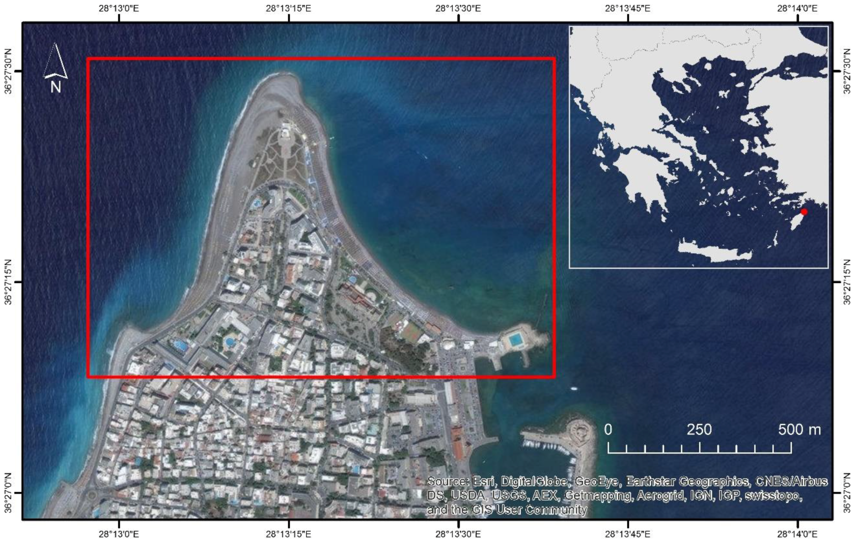
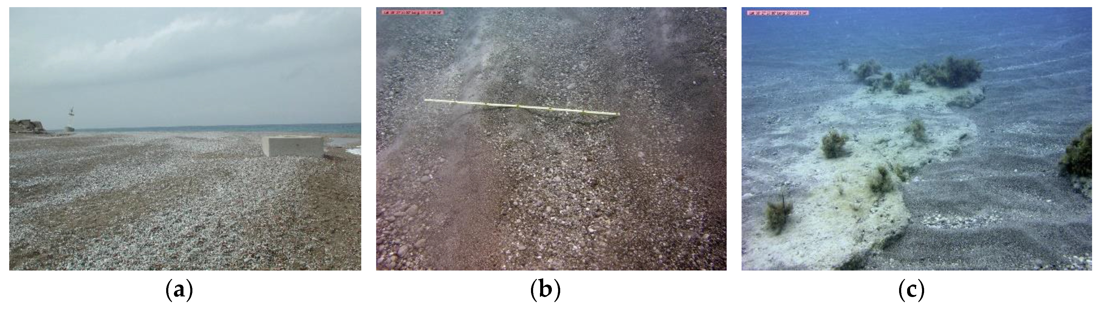
2. The Study Area
3. Materials and Methods
3.1. Analysis of Shoreline Evolution
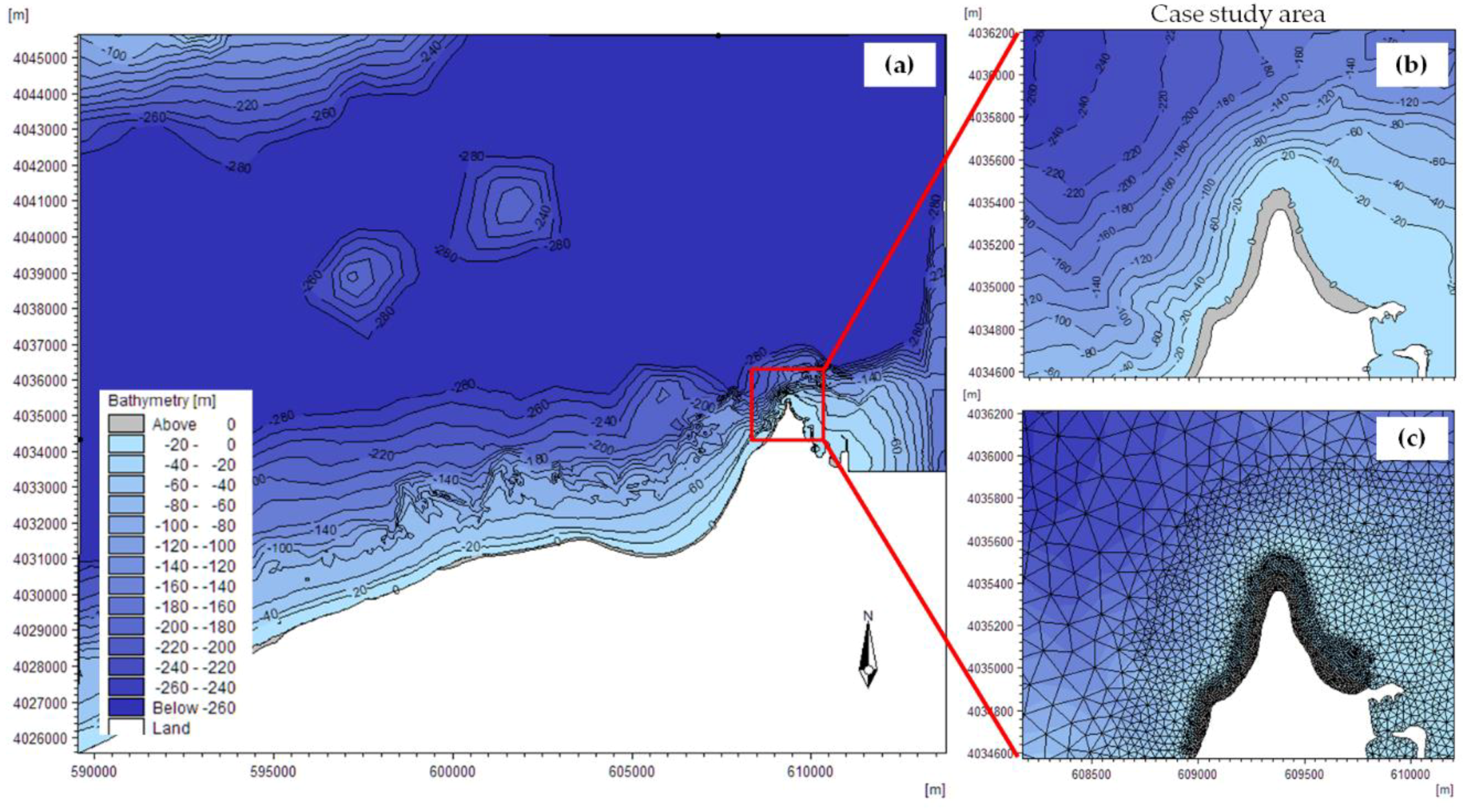
3.2. Simulation of Coastal Processes
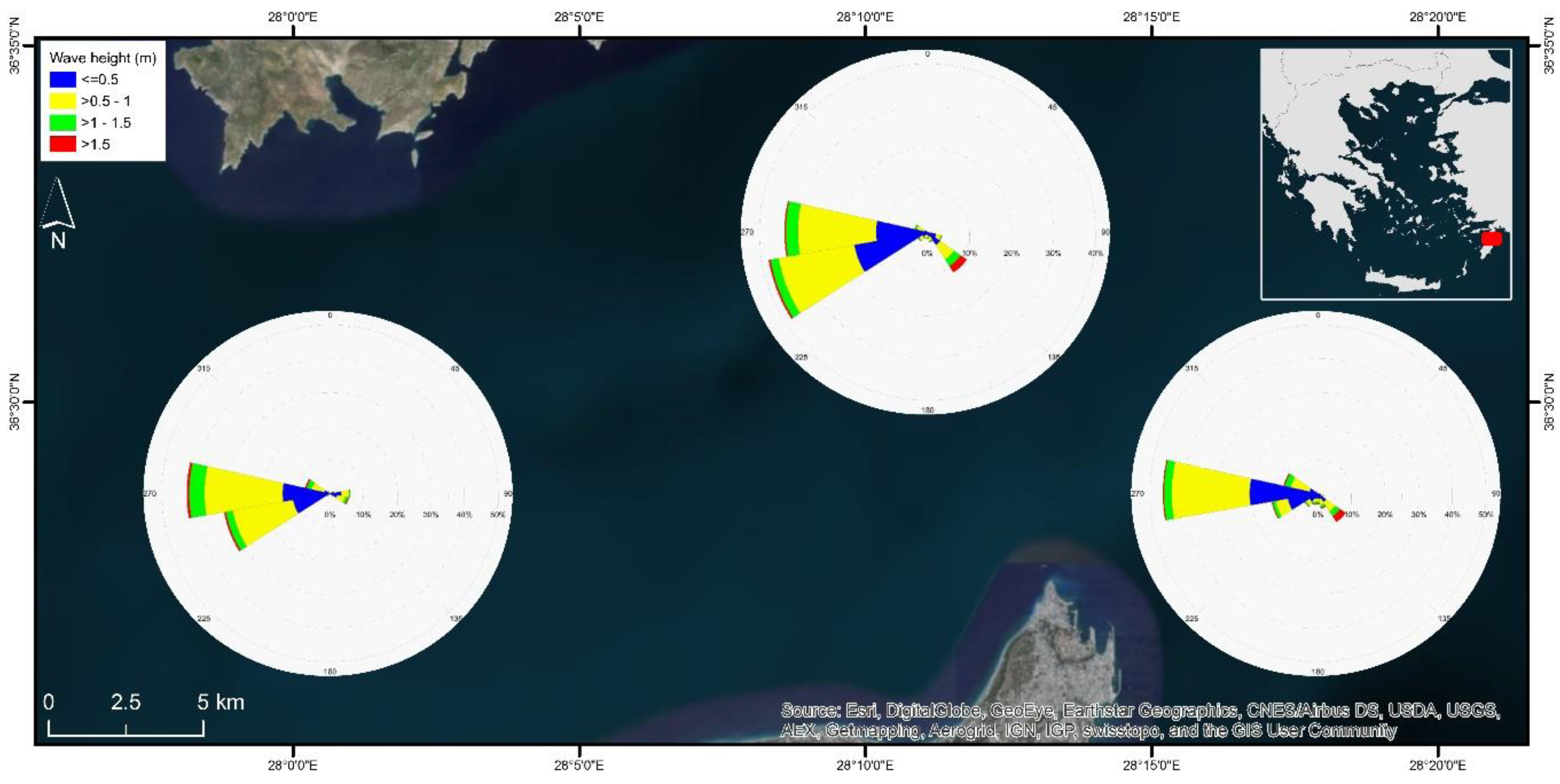
- Data are grouped into wave classes with associated annual probability of occurrence. Then, the actual energy flux is determined as fiHi2Ti, where Hi is the wave significant height, Ti is the wave period and fi denotes the probability of occurrence of the specific event, i.
- As representative event is defined the one that maximizes the energy flux and its probability of occurrence is determined asfmax = Σ(fi Ηi2 Ti)/(Ηi2 Ti)max
4. Results
4.1. Historical Shoreline Evolution
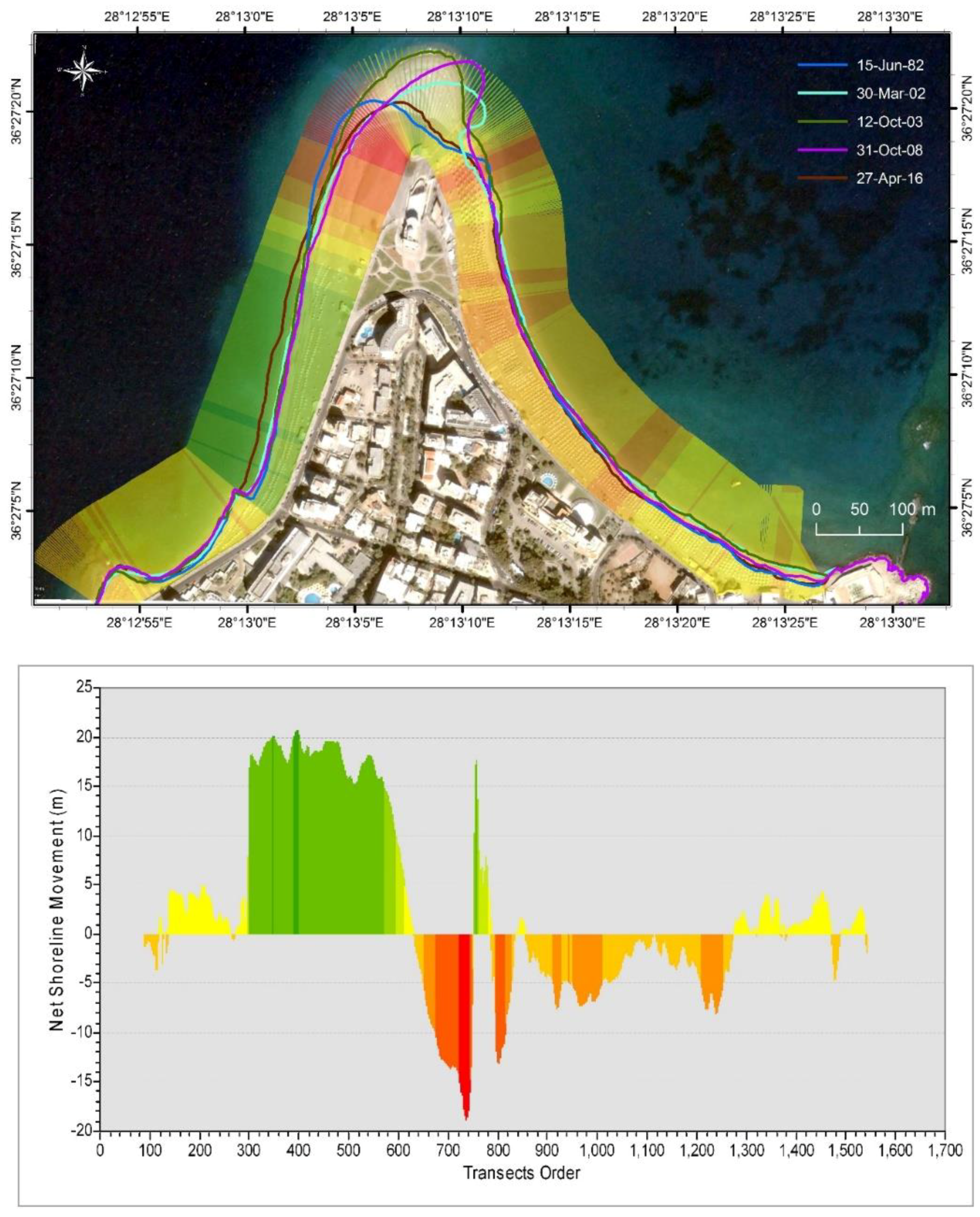
4.2. Morphodynamic Pattern
5. Discussion
6. Conclusions
Author Contributions
Funding
Acknowledgments
Conflicts of Interest
References
- Dan, S.; Stive, M.J.F.; Walstra, D.-J.R.; Panin, N. Wave climate, coastal sediment budget and shoreline changes for the Danube Delta. Mar. Geol. 2009, 262, 39–49. [Google Scholar] [CrossRef]
- Kaliraj, S.; Chandrasekar, N.; Magesh, N.S. Impacts of wave energy and littoral currents on shoreline erosion/accretion along the south-west coast of Kanyakumari, Tamil Nadu using DSAS and geospatial technology. Environ. Earth Sci. 2014, 71, 4523–4542. [Google Scholar] [CrossRef]
- Komar, P.D. Beach Processes and Sedimentation, 2nd ed.; Prentice Hall: Upper Saddle River, NJ, USA, 1998. [Google Scholar]
- Dalrymple, R.A.; MacMahan, J.H.; Reniers, A.J.H.M.; Nelko, V. Rip currents. Annu. Rev. Fluid Mech. 2011, 43, 551–581. [Google Scholar] [CrossRef]
- Leatherman, S.P.; Zhang, K.; Douglas, B.C. Sea level rise shown to drive coastal erosion. Eos. Trans. Am. Geophys. Union 2000, 81, 55–57. [Google Scholar] [CrossRef]
- Williams, S.J. Sea-level rise implications for coastal regions. J. Coast. Res. 2013, 63, 184–196. [Google Scholar] [CrossRef]
- Bray, M.J.; Carter, D.J.; Hooke, J.M. Littoral cell definition and budgets for central southern England. J. Coast. Res. 1995, 381–400. [Google Scholar]
- Hapke, C.J.; Lentz, E.E.; Gayes, P.T.; McCoy, C.A.; Hehre, R.; Schwab, W.C.; Williams, S.J. A review of sediment budget imbalances along Fire Island, New York: Can nearshore geologic framework and patterns of shoreline change explain the deficit? J. Coast. Res. 2010, 510–522. [Google Scholar] [CrossRef]
- Cowell, P.J.; Thom, B.G. Morphodynamics of Coastal Evolution; Cambridge University Press: Cambridge, UK; New York, NY, USA, 1994. [Google Scholar]
- Bird, E.C.F. Coastal Geomorphology: An Introduction; John Wiley & Sons: New York, NY, USA, 2011; ISBN 1119964350. [Google Scholar]
- Woodroffe, C.D. Coasts: Form, Process and Evolution; Cambridge University Press: New York, NY, USA, 2002; ISBN 0521011833. [Google Scholar]
- Lambeck, K.; Antonioli, F.; Anzidei, M.; Ferranti, L.; Leoni, G.; Scicchitano, G.; Silenzi, S. Sea level change along the Italian coast during the Holocene and projections for the future. Quat. Int. 2011, 232, 250–257. [Google Scholar] [CrossRef]
- Kapsimalis, V.; Poulos, S.E.; Karageorgis, A.P.; Pavlakis, P.; Collins, M. Recent evolution of a Mediterranean deltaic coastal zone: Human impacts on the Inner Thermaikos Gulf, NW Aegean Sea. J. Geol. Soc. London 2005, 162, 897–908. [Google Scholar] [CrossRef]
- Aouiche, I.; Daoudi, L.; Anthony, E.J.; Sedrati, M.; Ziane, E.; Harti, A.; Dussouillez, P. Anthropogenic effects on shoreface and shoreline changes: Input from a multi-method analysis, Agadir Bay, Morocco. Geomorphology 2016, 254, 16–31. [Google Scholar] [CrossRef]
- David, T.I.; Mukesh, M.V.; Kumaravel, S.; Sabeen, H.M. Long-and short-term variations in shore morphology of Van Island in gulf of Mannar using remote sensing images and DSAS analysis. Arab. J. Geosci. 2016, 9, 756. [Google Scholar] [CrossRef]
- Ashton, A.D.; Murray, A.B. High angle wave instability and emergent shoreline shapes: 1. Modeling of sand waves, flying spits, and capes. J. Geophys. Res. Earth Surf. 2006, 111, F4. [Google Scholar] [CrossRef]
- Berthot, A.; Pattiaratchi, C. Mechanisms for the formation of headland-associated linear sandbanks. Cont. Shelf Res. 2006, 26, 987–1004. [Google Scholar] [CrossRef]
- Thomas, T.; Lynch, S.K.; Phillips, M.R.; Williams, A.T. Long-term evolution of a sand spit, physical forcing and links to coastal flooding. Appl. Geogr. 2014, 53, 187–201. [Google Scholar] [CrossRef]
- Goodwin, I.D.; Freeman, R.; Blackmore, K. An insight into headland sand bypassing and wave climate variability from shoreface bathymetric change at Byron Bay, New South Wales, Australia. Mar. Geol. 2013, 341, 29–45. [Google Scholar] [CrossRef]
- Bastos, A.; Collins, M.; Kenyon, N. Water and sediment movement around a coastal headland: Portland Bill, Southern UK. Ocean Dyn. 2003, 53, 309–321. [Google Scholar] [CrossRef]
- Ashton, A.D.; Nienhuis, J.; Ells, K. On a neck, on a spit: Controls on the shape of free spits. Earth Surf. Dyn. 2016, 4, 193. [Google Scholar] [CrossRef]
- Kumar, A.; Narayana, A.C.; Jayappa, K.S. Shoreline changes and morphology of spits along southern Karnataka, west coast of India: A remote sensing and statistics-based approach. Geomorphology 2010, 120, 133–152. [Google Scholar] [CrossRef]
- Thomas, T.; Phillips, M.R.; Williams, A.T. Mesoscale evolution of a headland bay: Beach rotation processes. Geomorphology 2010, 123, 129–141. [Google Scholar] [CrossRef]
- Esteves, L.S.; Williams, J.J.; Dillenburg, S.R. Seasonal and interannual influences on the patterns of shoreline changes in Rio Grande do Sul, southern Brazil. J. Coast. Res. 2006, 1076–1093. [Google Scholar] [CrossRef]
- Pethick, J.S.; Crooks, S. Development of a coastal vulnerability index: A geomorphological perspective. Environ. Conserv. 2000, 27, 359–367. [Google Scholar] [CrossRef]
- Boak, E.H.; Turner, I.L. Shoreline definition and detection: A review. J. Coast. Res. 2005, 688–703. [Google Scholar] [CrossRef]
- Lakhan, V.C. Advances in Coastal Modeling. Elsevier Oceanography Series; Elsevier Science & Technology: New York, NY, USA, 2003; ISBN 1281054801. [Google Scholar]
- Guillou, N.; Chapalain, G. Effects of waves on the initiation of headland-associated sandbanks. Cont. Shelf Res. 2011, 31, 1202–1213. [Google Scholar] [CrossRef]
- Belibassakis, K.A.; Karathanasi, F.E. Modelling nearshore hydrodynamics and circulation under the impact of high waves at the coast of Varkiza in Saronic-Athens Gulf. Oceanologia 2017, 59, 350–364. [Google Scholar] [CrossRef] [Green Version]
- Martinez, J.O.; Pilkey, O.H.; Neal, W.J. Rapid formation of large coastal sand bodies after emplacement of Magdalena river jetties, Northern Colombia. Environ. Geol. Water Sci. 1990, 16, 187–194. [Google Scholar] [CrossRef]
- Anagnostou, C.; Antoniou, P.F.; Hatiris, G.A. Erosion of a depositional coast in NE Rhodos island (SE Greece) and assessment of the best available measures for coast protection. J. Coast. Res. 2011, 64, 1316–1319. [Google Scholar]
- Hatiris, G.A.; Kapsimalis, V.; Rousakis, G.; Panagiotopoulos, I.; Kyriakidou, H.; Morfis, I.; Kondylatos, G.; Anagnostou, C.; Sioulas, A. Morphometric Characteristics of Submarine Canyons on the Eastern Continental Shelf of Rhodes Island and İnsights on Their Generating Mechanisms. In Proceedings of the 11th Panhellenic Symposium of Oceanography & Fisheries, Mytilene, Greece, 13–17 May 2015. [Google Scholar]
- Verikiou-Papaspiridakou, E.; Bathrellos, G.; Skilodikou, H. Physico-geographical observations of the coastal zone of the northeastern part of Island Rhodes. Bull. Geol. Soc. Greece 2004, 36, 958–967. [Google Scholar]
- Kombiadou, K.; Chatiris, G.A.; Androulidakis, G.; Sioulas, A.; Krestenitis, G.; Anagnostou, C.; Issaris, G. Investigation of erosion at the cape of Rhodos and defence measures. In Proceedings of the 9th Symposium on Oceanography & Fisheries, Patras, Greece, 13–16 May 2009; Volume 1, pp. 178–183. [Google Scholar]
- Soukissian, T.; Hatzinaki, M.; Korres, G.; Papadopoulos, A.; Kallos, G.; Anadranistakis, E. Wind and Wave Atlas of the Hellenic Seas; Hellenic Centre for Marine Research: Anavyssos, Greece, 2007; ISBN 978960866519-4. [Google Scholar]
- Hellenic Hydrographic Service. Statistical Data of Sea Level at Greek Ports; Hydrographic Service, Hellenic Army Navy: Athens, Greece, 2013. [Google Scholar]
- Pytharouli, S.I.; Stiros, S.C. Analysis of short and discontinuous tidal data: A case study from the Aegean Sea. Surv. Rev. 2012, 44, 239–246. [Google Scholar] [CrossRef]
- Google Earth V 7.3.1.4507. Cape Mylon, Rhodes, Greece. Lat: 36.455364N, Lon: 28.220384E. Eye alt 897 m. DigitalGlobe 30/03/2002-03/09/2012 & 14/05/2014-21/04/2016, CNES/Airbus 09/10/2013 & 27/04/2016. Available online: http://www.google.com/earth (accessed on 3 September 2016).
- Di Stefano, A.; De Pietro, R.; Monaco, C.; Zanini, A. Anthropogenic influence on coastal evolution: A case history from the Catania Gulf shoreline (eastern Sicily, Italy). Ocean Coast. Manag. 2013, 80, 133–148. [Google Scholar] [CrossRef]
- Malarvizhi, K.; Kumar, S.V.; Porchelvan, P. Use of High Resolution Google Earth Satellite Imagery in Landuse Map Preparation for Urban Related Applications. Procedia Technol. 2016, 24, 1835–1842. [Google Scholar] [CrossRef]
- Martin, D.; Jones, R. What Transformation ? Appropriate Transformations for Georeferencing Scanned Maps in ArcGIS; Helyx Secure information Systems Ltd.: Gloucestershire, UK, 2015; p. 23. [Google Scholar]
- Nave, S.; Rebêlo, L. High-resolution geological cartography and coastal evolution assessment at Armação de Pêra–Galé sector: A prototype for a national coastal mapping. J. Coast. Conserv. 2018, 1–13. [Google Scholar] [CrossRef]
- Morton, R.A. National Assessment of Shoreline Change: Part 1: Historical Shoreline Changes and Associated Coastal Land Loss along the US Gulf of Mexico; Diane Publishing: Darby, PA, USA, 2008; ISBN 1437902596. [Google Scholar]
- Fletcher, C.H.; Romine, B.M.; Genz, A.S.; Barbee, M.M.; Dyer, M.; Anderson, T.R.; Lim, S.C.; Vitousek, S.; Bochicchio, C.; Richmond, B.M. National Assessment of Shoreline Change: Historical Shoreline Change in the Hawaiian Islands; Open-File Report 2011–1051; U.S. Geological Survey: Reston, Virginia, USA, 2011.
- Thieler, E.R.; Himmelstoss, E.A.; Zichichi, J.L.; Ergul, A. The Digital Shoreline Analysis System (DSAS) Version 4.0-An ArcGIS Extension for Calculating Shoreline Change; US Geological Survey: Tallahassee, FL, USA, 2009.
- DHI. MIKE 21/3 Coupled Model FM, User Guide; Danish Hydraulic Institute: Hørsholm, Denmark, 2016. [Google Scholar]
- US Army Corps of Engineers. Chapter III-2, Longshore Sediment Transport, Engineer Manual 1110-2-1100. In US Army Corps of Engineers (USACE) Coastal Engineering Manual; US Army Corps of Engineers: Washington, DC, USA, 2006. [Google Scholar]
- Borah, D.K.; Balloffet, A. Beach evolution caused by littoral drift barrier. J. Waterw. Port Coast. Ocean Eng. 1985, 111, 645–660. [Google Scholar] [CrossRef]
- López-Ruiz, A.; Ortega-Sánchez, M.; Baquerizo, A.; Losada, M.A. Short and medium-term evolution of shoreline undulations on curvilinear coasts. Geomorphology 2012, 159, 189–200. [Google Scholar] [CrossRef]
- López-Ruiz, A.; Ortega-Sánchez, M.; Baquerizo, A.; Losada, M.Á. A note on alongshore sediment transport on weakly curvilinear coasts and its implications. Coast. Eng. 2014, 88, 143–153. [Google Scholar] [CrossRef]
- Park, J.-Y.; Wells, J.T. Longshore transport at Cape Lookout, North Carolina: Shoal evolution and the regional sediment budget. J. Coast. Res. 2005, 1–17. [Google Scholar] [CrossRef]
- Martínez, C.; Quezada, M.; Rubio, P. Historical changes in the shoreline and littoral processes on a headland bay beach in central Chile. Geomorphology 2011, 135, 80–96. [Google Scholar] [CrossRef]
- Sánchez-Arcilla, A.; Jiménez, J.A. Breaching in a wave-dominated barrier spit: The trabucador bar (north-eastern spanish coast). Earth Surf. Process. Landf. 1994, 19, 483–498. [Google Scholar] [CrossRef]
- Patsch, K.; Griggs, G. Littoral Cells, Sand Budgets, and Beaches: Understanding California’s Shoreline; Institute of Marine Sciences: Santa Cruz, CA, USA, 2006. [Google Scholar]
- Karambas, T.V; Samaras, A.G. Soft shore protection methods: The use of advanced numerical models in the evaluation of beach nourishment. Ocean Eng. 2014, 92, 129–136. [Google Scholar] [CrossRef]


| Date | Type | Source | Scale/Resolution |
|---|---|---|---|
| 15 June 1982 | Aerial photograph | Hellenic Military Geographical Service | 1:8000 |
| 17 June 1991 | Aerial photograph | Hellenic Military Geographical Service | 1:8000 |
| 30 March 2002 | Satellite Imagery | QuickBird-2 | 67.28 cm |
| 12 October 2003 | Satellite Imagery | QuickBird-2 | 62.59 cm |
| 31 October 2008 | Satellite Imagery | Orthophotomaps of the Hellenic Cadastre | 50.00 cm |
| 22 April 2009 | Satellite Imagery | GeoEye-1 | 43.51 cm |
| 16 July 2010 | Satellite Imagery | GeoEye-1 | 42.99 cm |
| 30 May 2012 | Satellite Imagery | WorldView-2 | 47.28 cm |
| 3 September 2012 | Satellite Imagery | GeoEye-1 | 44.76 cm |
| 9 October 2013 | Satellite Imagery | Pléiades-1A | 50 cm |
| 14 May 2014 | Satellite Imagery | WorldView-2 | 55.34 cm |
| 29 June 2014 | Satellite Imagery | WorldView-2 | 47.72 cm |
| 17 August 2014 | Satellite Imagery | WorldView-2 | 47.88 cm |
| 2 October 2014 | Satellite Imagery | WorldView-2 | 47.77 cm |
| 16 March 2015 | Satellite Imagery | GeoEye-1 | 47.22 cm |
| 17 October 2015 | Satellite Imagery | WorldView-3 | 33.61 cm |
| 21 April 2016 | Satellite Imagery | WorldView-2 | 48.24 cm |
| 27 April 2016 | Satellite Imagery | Pléiades-1A | 50 cm |
| Scenarios | Hs (m) | Tp (s) | MWD (deg N) | Simulation Time (days) |
|---|---|---|---|---|
| Sc1 | 1.25 | 6.75 | 255 | 45 |
| Sc2 | 1.25 | 5.25 | 270 | 39 |
| Sc3 | 2.25 | 6.75 | 135 | 12 |
| Sc4 | 1.75 | 5.25 | 300 | 4 |
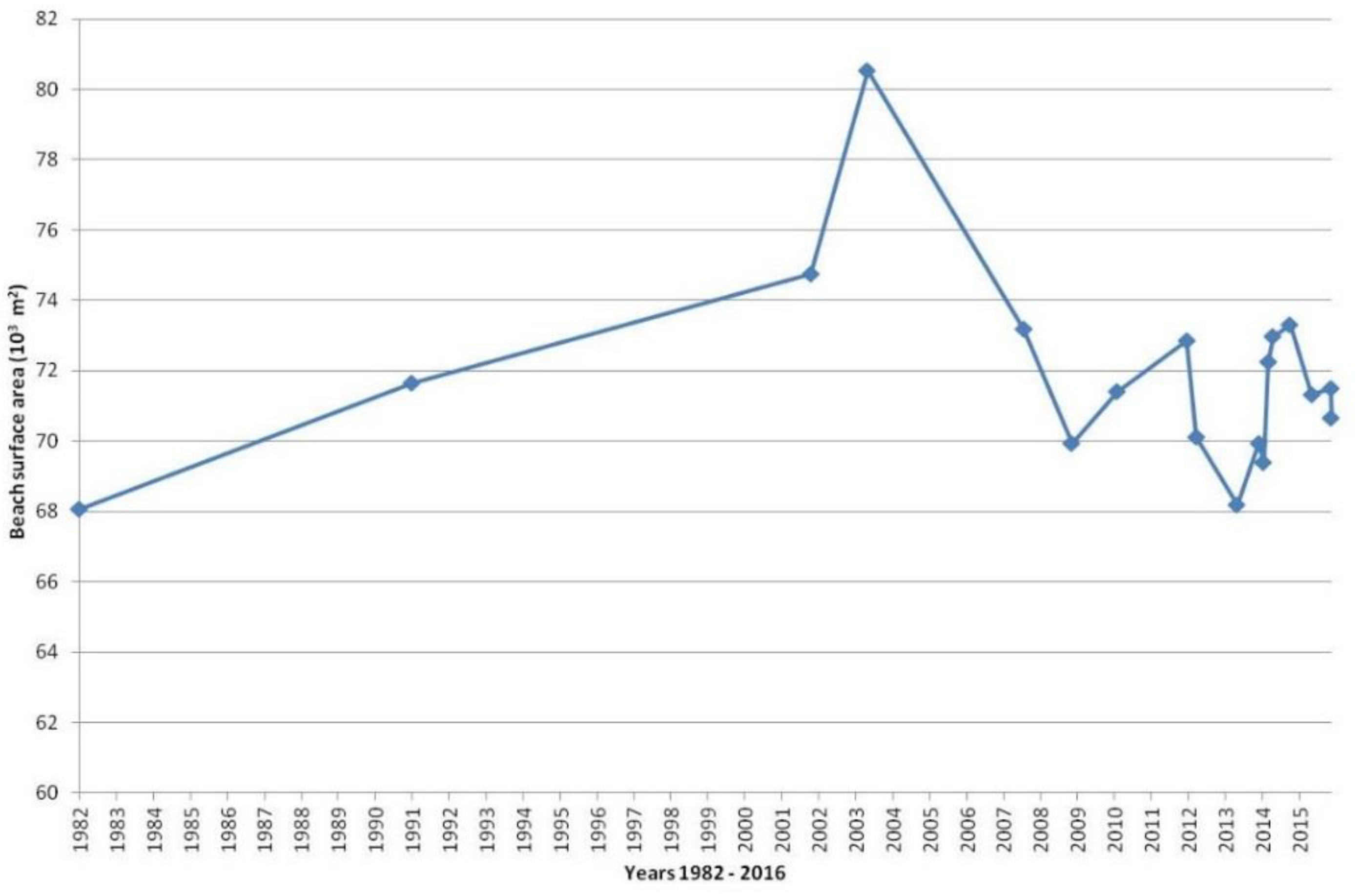
| Shoreline | Max Advance (m) | Max Retreat (m) | Coastal Zone Surface (m2) | Surface Evolution between Consecutive Shoreline Items (m2) | Cumulative Surface Evolution (from 1982) (m2) | Duration (y) |
|---|---|---|---|---|---|---|
| 15 June 1982 | Shoreline of reference | 68,056.6 | Shoreline of reference | |||
| 17 June 1991 | 40.9 | −15.5 | 71,651.9 | 3595.3 | 3595.3 | 9.01 |
| 30 March 2002 | 69.9 | −25.1 | 74,759.5 | 3107.6 | 6702.9 | 19.79 |
| 12 October 2003 | 91.6 | −20.0 | 80,526.8 | 5767.3 | 12,470.2 | 21.33 |
| 31 October 2008 | 97.1 | −25.4 | 73,191.4 | −7335.4 | 5134.7 | 25.54 |
| 22 April 2009 | 27.1 | −32.4 | 69,941.0 | −3250.4 | 1884.4 | 26.85 |
| 16 July 2010 | 59.0 | −25.0 | 71,413.9 | 1472.9 | 3357.3 | 28.09 |
| 30 May 2012 | 39.8 | −16.9 | 72,864.6 | 1450.8 | 4808.0 | 29.96 |
| 3 September 2012 | 51.2 | −17.1 | 70,106.3 | −2758.4 | 2049.7 | 30.22 |
| 9 October 2013 | 61.5 | −21.9 | 68,199.3 | −1906.9 | 142.7 | 31.32 |
| 14 May 2014 | 37.8 | −33.9 | 69,923.7 | 1724.4 | 1867.1 | 31.91 |
| 29 June 2014 | 28.2 | −31.2 | 69,397.3 | −526.4 | 1340.7 | 32.04 |
| 17 August 2014 | 46.1 | −25.6 | 72,241.0 | 2843.7 | 4184.4 | 32.17 |
| 2 October 2014 | 57.3 | −29.7 | 72,967.5 | 726.5 | 4910.9 | 32.30 |
| 16 March 2015 | 40.5 | −34.9 | 73,291.5 | 324.0 | 5234.9 | 32.75 |
| 17 October 2015 | 64.7 | −28.8 | 71,329.4 | −1962.1 | 3272.8 | 33.34 |
| 21 April 2016 | 21.7 | −17.0 | 71,484.1 | 154.7 | 3427.5 | 33.85 |
| 27 April 2016 | 20.8 | −18.9 | 70,655.0 | −829.1 | 2598.4 | 33.87 |
© 2018 by the authors. Licensee MDPI, Basel, Switzerland. This article is an open access article distributed under the terms and conditions of the Creative Commons Attribution (CC BY) license (http://creativecommons.org/licenses/by/4.0/).
Share and Cite
Gad, F.-K.; Hatiris, G.-A.; Loukaidi, V.; Dimitriadou, S.; Drakopoulou, P.; Sioulas, A.; Kapsimalis, V. Long-Term Shoreline Displacements and Coastal Morphodynamic Pattern of North Rhodes Island, Greece. Water 2018, 10, 849. https://doi.org/10.3390/w10070849
Gad F-K, Hatiris G-A, Loukaidi V, Dimitriadou S, Drakopoulou P, Sioulas A, Kapsimalis V. Long-Term Shoreline Displacements and Coastal Morphodynamic Pattern of North Rhodes Island, Greece. Water. 2018; 10(7):849. https://doi.org/10.3390/w10070849
Chicago/Turabian StyleGad, Fragkiska-Karmela, Giorgos-Angelos Hatiris, Vassiliki Loukaidi, Stavroula Dimitriadou, Paraskevi Drakopoulou, Andreas Sioulas, and Vasilios Kapsimalis. 2018. "Long-Term Shoreline Displacements and Coastal Morphodynamic Pattern of North Rhodes Island, Greece" Water 10, no. 7: 849. https://doi.org/10.3390/w10070849