The Impact of Multiple Typhoons on Severe Floods in the Mid-Latitude Region (Hokkaido)


Institute for Rural Engineering, National Agriculture and Food Research Organization (NARO), 2-1-6 Kannondai, Tukuba, Ibaraki 305-8609, Japan
*
Author to whom correspondence should be addressed.
Water 2018, 10(7), 843; https://doi.org/10.3390/w10070843
Submission received: 16 May 2018
/
Revised: 14 June 2018
/
Accepted: 20 June 2018
/
Published: 25 June 2018
(This article belongs to the Special Issue The Application of Hydrologic Analysis in Disaster Prevention)
Abstract
:Mid-latitude regions in the North Pacific are generally vulnerable to climatological disasters and are possibly more sensitive to future climate changes. Severe flood disasters struck Hokkaido in August 2016 because of the multiple, continuous typhoons that struck the island. We evaluated the effect of these typhoons on floods and changes in future floods using a distributed hydrological model in a watershed located in eastern Hokkaido. We conducted two numerical examinations: a simulation with a major typhoon only (which caused flood disasters) without other preceding typhoons, and a simulation with a simple assumed future climate (in which we employed higher precipitation). The result of the former simulation demonstrated that the impact of the preceding typhoons on the highest flood peak was significant during the early stage of the major typhoon but weaker after the middle stage of the major typhoon. The result of the latter simulation indicated that flood peaks potentially increased with an increase in precipitation. Based on the water level distributions in the surface layer, the impact of multiple typhoons and future weather conditions on potential flood peaks depends on the degree of soil saturation over our target watershed.
1. Introduction
Inlands and islands in the mid-latitude of the North Pacific have limited experience with typhoon-induced hazards. These regions in general are vulnerable to heavy rain-induced flood disasters because it is difficult for a strong-intensity typhoon to reach them. For instance, Hokkaido (the northern island of Japan, 41.35–45.56° N, 139.33–148.89° E) experienced typhoon attacks and approaches a few times a year from 1961 to 2016 according to the Japan Meteorological Agency (JMA) [1]. Typhoon-induced flood disasters in the mid-latitude areas of the Korean Peninsula have historically occurred (e.g., Myeong and Hong [2]), probably owing to weak infrastructure and excessive agricultural development, but the frequency of the flood disasters was limited to approximately once a year. Therefore, past studies associated with typhoon hazards in the mid-latitude regions [3,4] are few.
The Intergovernmental Panel on Climate Change (IPCC) reported that severe natural disasters due to climate extremes have occurred more often since 2000 AR4 [5]. Future climate extremes caused by global warming may enhance heavy rainfall events in the mid-latitude regions [4] significantly changing the mid-latitude climate according to the IPCC Fourth Assessment Report (AR4) [6]. The frequency of heavy rain events with over 240 mm of rainfall for three days may dramatically increase during the summer in Hokkaido [7]. The available studies imply that even in the mid-latitude regions the number of typhoons may increase in the future and multiple continuous typhoons may occur.
In reality, scenarios that were expected to occur in the future have already occurred in mid-latitude regions. Four typhoons—Chanthu, Kompasu, Mindulle, and Lionrock (Table 1)—which consecutively struck Hokkaido in August 2016 caused enormous damage (this is hereafter referred to as the August 2016 disaster). In addition to life and property losses (approximately 260 million USD), these four typhoons caused agricultural damage (40,258 ha) all over Hokkaido [8]. Potential reasons for this damage are as follows: four typhoons continuously reached Hokkaido within a short period; the fourth typhoon (Typhoon Lionrock), which had an unusual passage from the North Pacific to the Sea of Japan, was of strong intensity (Category 4 with winds of 225 km/h); and most of the land in Hokkaido is farmland, which is usually vulnerable to typhoon hazards [8].
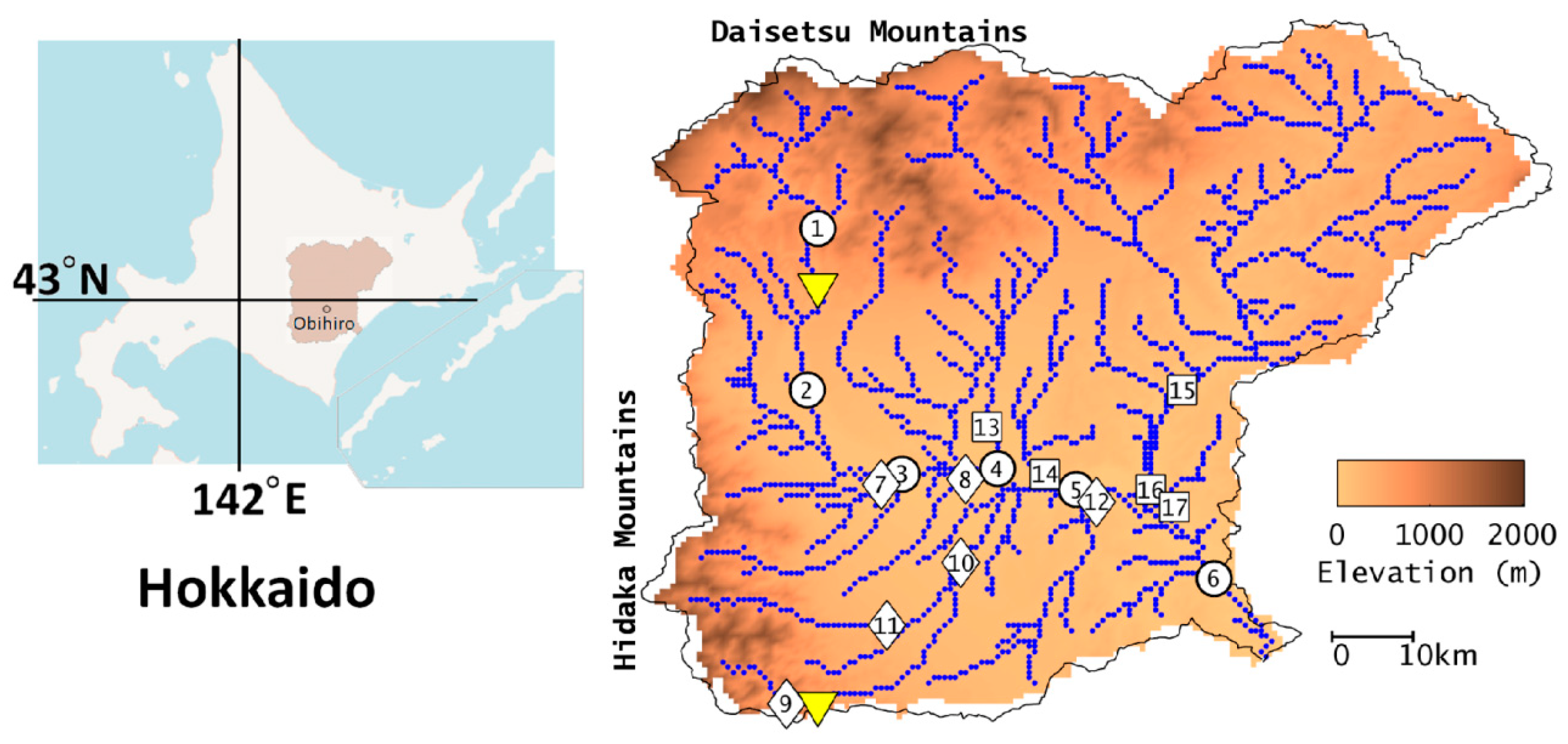
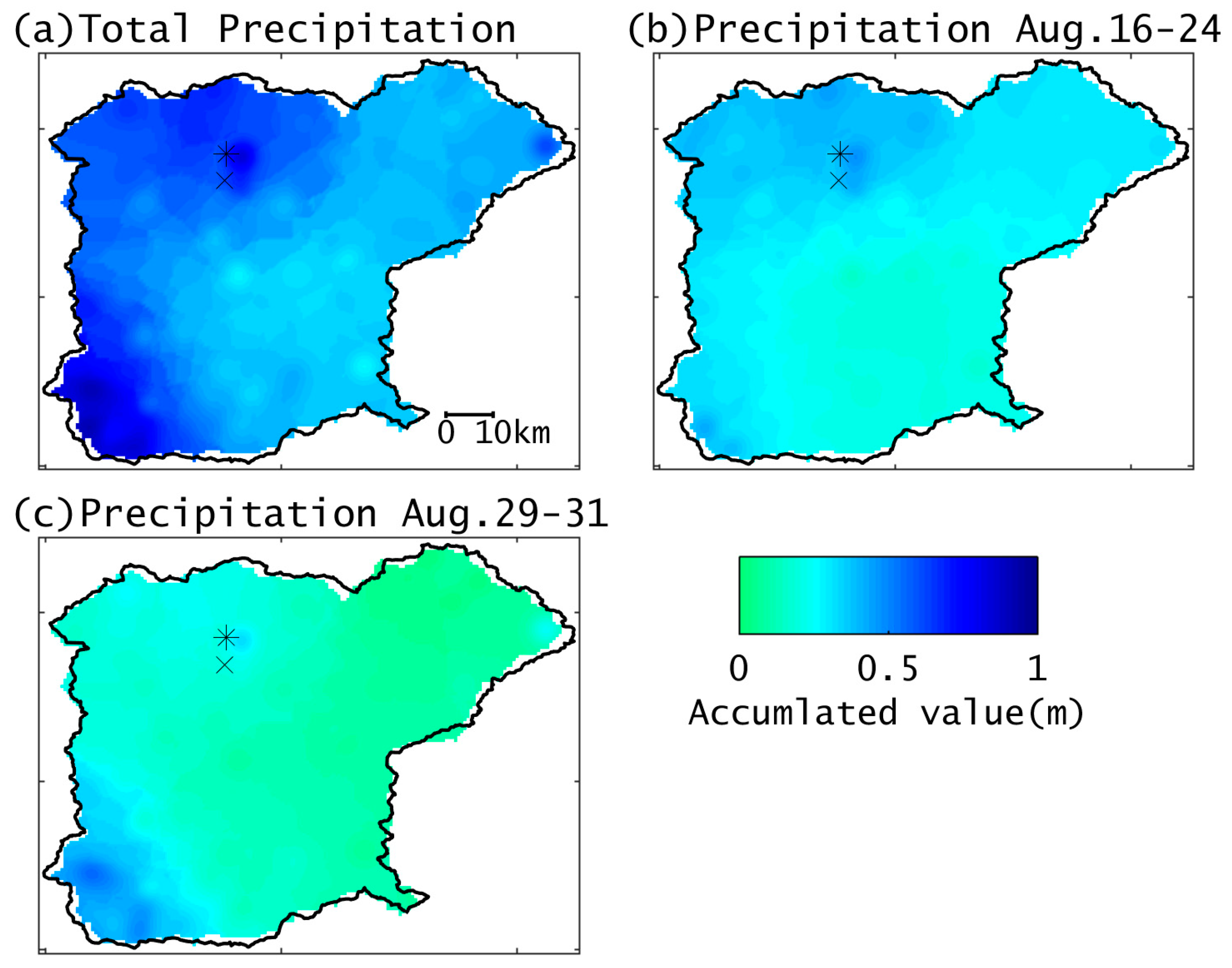
In the August 2016 disaster, we targeted one of the flood-damaged areas, the Tokachi River (TR) watershed (42.54–43.64° N, 142.68–144.03° E) located in the southeast region of Hokkaido (Figure 1) because upland fields are dominant over the watershed. Heavy rainfall events occurred from 16–24 August when the preceding three typhoons struck (e.g., >400 mm according to the Naitai station rain gage), according to the water resource database provided by the Ministry of Land, Infrastructure, Transport, and Tourism of Japan (MLIT Japan) [9]. Then, the fourth typhoon, Typhoon Lionrock, on 29–31 August passed the south of Hokkaido and brought heavy rainfall (>200 mm according to the Naitai station rain gage) over the westside of the Hidaka Mountains (southeast Hokkaido) and around the Daisetsu Mountains (central Hokkaido). For atmosphere dynamics, the raincloud hit the Hidaka Mountains from the west, and then the upward movement of air brought approximately 500 mm of precipitation for 48 h to the Satsunai River Dam station near the Hidaka Mountains. This evidence suggested that mountain-induced orographic rainfall occurred [8]. In particular, floods in the main stream and nine tributaries of the TR severely damaged agricultural and city areas (e.g., inundation of approximately 912 ha, loss of 15 houses, over 150 houses inundated above/below floor level) and infrastructure (e.g., several dyke and bridge collapses) mainly in the west portion of the TR watershed [10]. Significant landsides that occurred in several tributaries over the western TR watershed also were also confirmed [11]. Soil was already saturated in a small sub-watershed of the TR watershed during the preceding three typhoons [12]. This severe disaster may have occurred because the impact of the fourth typhoon approach was so considerable that infiltration into the ground was insufficient as the heavy rainfall brought by the leading three typhoons had saturated the soil. However, a quantitative assessment of the entire TR watershed is not likely to have been reported yet. Therefore, we focused on understanding the effect of the leading three typhoons on severe flood occurrences during the approach of Typhoon Lionrock.
To evaluate the impact of multiple typhoons (which hit the same area within a short period) on flood-induced damage in a mid-latitude region, we validate a flood model applied to a severely damaged watershed in the August 2016 disaster, conduct an artificial numerical examination to measure the flood severity between multiple typhoon and single typhoon attacks, and further perform another examination to estimate future multiple floods that may often occur in future extreme weather conditions that are presumably similar to those of the August 2016 disaster.
2. Methods
2.1. Target Site
Our study site is the TR watershed, located in the eastern portion of Hokkaido. The watershed shape resembles that of a fan; the area is approximately 9010 km2. The longest river is approximately 156 km long, passing through an urban area (Obihiro) located on flat land and reaching the North Pacific from the east. The altitude ranges from 0 to 2077 m (Figure 1). Most low-plane areas are utilized as farmland. The countermeasures against severe floods are still poor, especially for middle-/small-tributaries, although a few dams for flood control exist in the upstream areas [13]. The hydraulic characteristics of the watershed are as follows: heavy rains usually occur in the high mountains, which stand at the west, north, and east boundaries of the TR watershed; the rain water gathers in the downstream area through the river network on the right and left sides of the watershed, and it is conveyed to the outlet (North Pacific). A time lag of several hours exists in the downstream area after heavy rainfall occurs in the upstream area. Robust countermeasures against flood hazards in the TR watershed will be required because of potential severe disasters due to future climate extremes in the mid-latitude regions [14].
2.2. Integrated Flood Analysis System
We performed several numerical examinations for floods in main and tributary rivers over TR watershed. We employed a comprehensive Graphical User Interface (GUI) operating runoff simulator, the Integrated Flood Analysis System (IFAS), possibly combined with satellite weather data. The IFAS was developed by the International Centre for water Hazard and Risk Management (ICHARM) [15,16], and has been practically applied to historical flood events all over the world by the United Nations Educational, Scientific and Cultural Organization (UNESCO) [17,18]. A conceptual, distributed rainfall-runoff analysis engine, the Public Works Research Institute-Distributed Hydrological Model (PWRI-DHM) [19], is embedded in the IFAS as one of the IFAS modules. Several coefficients in the PWRI-DHM are efficiently set up based on soil-type and land use features. For the IFAS computational conditions in the TR watershed, the number of cells was 170 × 137 in the horizontal direction over the entire watershed and each cell size was 0.008° × 0.008° in the World Geodetic System 1984 (WGS84). The river channel network over the watershed was determined by the altitude information.
2.3. Data Inputs
Our inputs for the IFAS hydrological information were the elevation, land use, and soil-geology data. The elevation data was obtained from the digital elevation model from the altitude information of the shuttle radar topography mission with a three arc-second resolution (approximately 90 m) in the hydrological data and maps based on shuttle elevation derivatives at multiple scales (HydroSHEDS) [20]. The land use data with a 1-km mesh resolution was downloaded from the website of the Global Land Cover Characterization (GLCC) website [21]; the data was collected in the U.S. Geology Survey. The data for the geology and soil type were obtained from the global distribution data for soil water holding capacity with a one-degree resolution at 0 to 0.3 m in the surface of the soil compiled as part of the United Nations Environment Programme. The observed rainfall data was obtained from MLIT Japan and the Japan Meteorological Agency (JMA) at approximately 50 gage stations as ground-based data (Figure 2). The other meteorological data, such as wind speed and shortwave radiation, were provided by the JMA. The water stage data were obtained from MLIT Japan. Those data are hourly data sets that can be accessed on the agency’s websites [9,22]. The rainfall input data were distributed into the several divisions of the watershed area using the ordinary kriging, which is a geostatistical interpolation that uses a least-squares regression method among neighborhood observations (Figure 2). Note that we performed interpolation/extrapolation for missing rainfall data because some rain gages were mechanically maintained or damaged by the preceding typhoons.
2.4. Simulation Preparations
For water movement from the surface to the river through precipitation, infiltration, and percolation processes, we employed a three-tank model incorporated with the Penman heat budget method for evapotranspiration in the PWRI-DHM [15] (Appendix A). For all parameters related to several hydrologic characteristics in the hydrological model, default values were employed. The observed discharges from Tokachi Dam and Satsunai River Dam, which were the two dams used for flood control (Table 2), were added to the model for the simulation period. The model also considered the effect of evaporation on discharge using the observed weather data (wind, humidity, air temperature and sunlight) and reduced the effect of the initial condition on saturated water in the soil using the mean precipitation (approximately 0.2 mm/h) in August over the past years as a spin-up process. For our assumptions, specific sub-models such as the water and sewage system in an urban area, the farmland irrigation system, and interception over forests were not implemented. The reasons are as follows: The urban area represents less than a few percent of the TR watershed, the farmland irrigation system is hardly utilized for flood control, and the effect of interception over forests is minor. Our study was designed for an extremely heavy rain event. Therefore, the influence of these sub-models can be ignored.
The observed water stage data of the rivers was utilized to validate the model. The IFAS provides river discharge () as output data. As the stage–discharge relationship at each gage station was not obtained, we converted the discharge data to water stage data () using Manning’s formula with some model parameters ( = roughness coefficient and = river gradient):
where is the actual length of the river cross section. The water stage at the start of the model simulation was set to 0 m (height).
2.5. Indicators for Model Validation
The root-mean-square error (RMSE) against the total quantity of observation data was used to compute reproducibility (Rp, %), similar to the relative RMSE, of the simulation result against discharge [23]. The equation is given by
where
In Equation (3), is the observed data, is the simulated data, is the number of points, and is the total variation in the difference between the observed value and zero value. Another indicator widely used to measure the accuracy of the output of the flood model is the Nash–Sutcliffe model efficiency coefficient (NS) [24], which is given by
where is the average value for the observed data. However, NS is in general applied to a single peak flood and is inappropriate for a relatively flat water stage because the differences between the observed values and the mean value of the second term of (4) are underestimated. Therefore, NS would have been inappropriate for evaluating a longer-term flood, including plural peaks, in our study, although it is shown here as a reference evaluation.
The mean absolute error (MAE) is also an effective indicator for measuring error, and is given by
3. Results
We first validated the hydrological simulation with the IFAS during 16 August to 5 September 2016, including the multiple typhoon attacks, using observed water stages, located in 17 gage stations (Figure 1), for which data were available for our simulation period and were appropriate for covering the main river and major tributaries. Then, we conducted a numerical examination to understand the impact of multiple typhoon attacks on the August 2016 disaster with or without the preceding typhoons. In addition, we discussed the impact of a future climate change scenario on a future flood using similar weather conditions as those of the August 2016 disaster.
3.1. Hydrological Model Validation
The validation of the PWRI-DHM, applied to the TR watershed during the August 2016 floods, was performed by comparing the simulated and observed water stages at gages on the main stream, the tributaries on the northern side (N-tributaries), and the tributaries on the southern side (S-tributaries) of the main stream. This simulated result for the actual event is named Case 1. The model did not consider flow loss from rivers due to the broken dykes because the flooding areas were within one grid scale, and an uncertainty analysis from observation designs, such as the number of rain gage stations and the appropriate locations of these stations, was beyond the scope of this study.
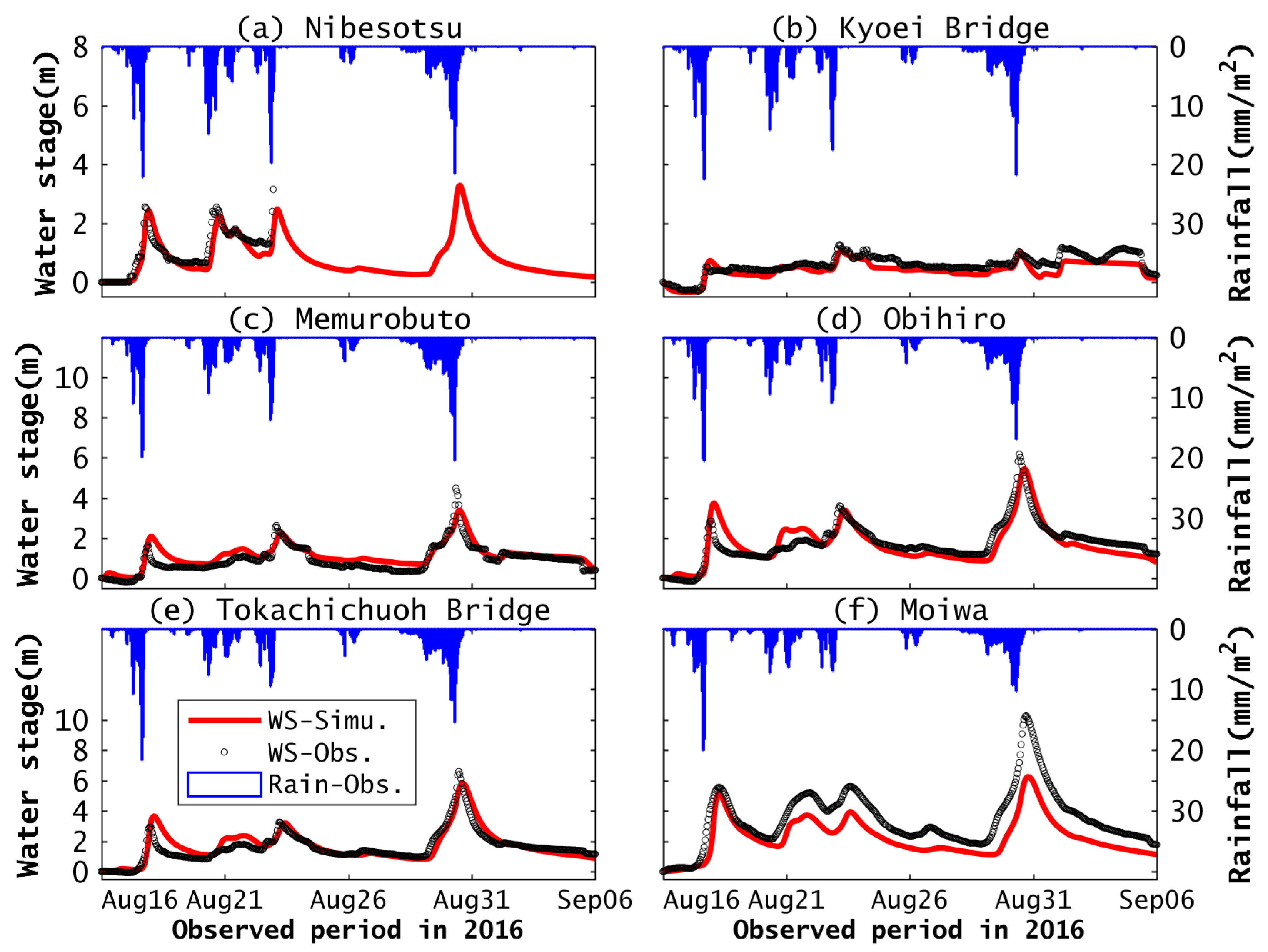
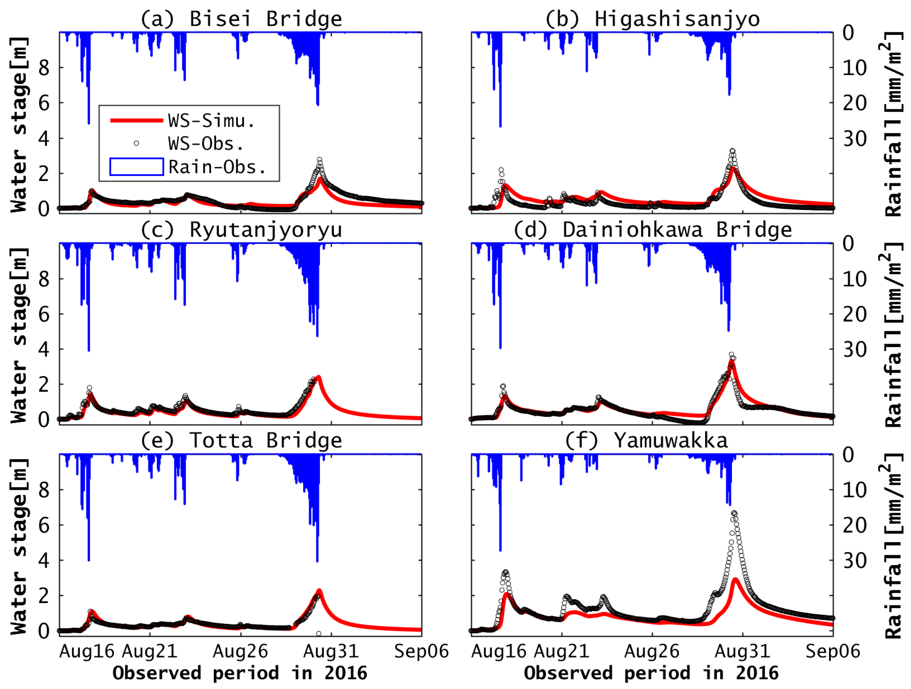
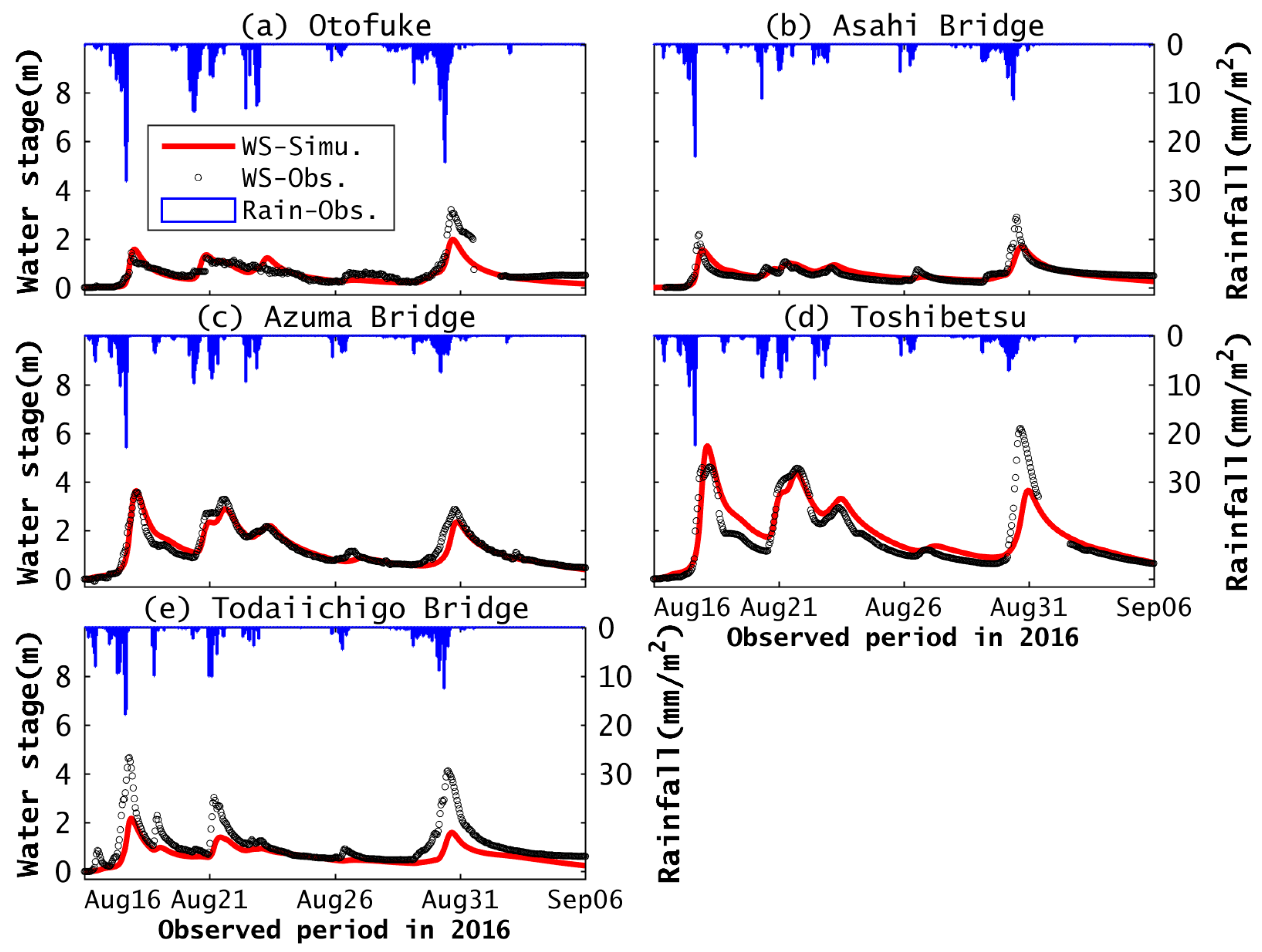
Simulated water stages along the main stream were highly similar to the observed water stages with an Rp of 0.63–0.76 (Figure 3, Table 3). In particular, the peaks were underestimated with an up to 40% reduction during the approach of Typhoon Lionrock on 29–31 August (hereafter Period II). These offsets of the simulated peaks might be attributed to missing rainfall data during Period II and sparse rain gage stations over the northwest mountain area in the TR watershed. Adaptive flood control, including a prior discharge and flood peak cut, by the Tokachi Dam successfully made the water stage flat during multiple typhoon attacks to reduce flood risk in the downstream area as shown in gage station 2 (Kyoei Bridge, hereafter Gage 2) close to Tokachi Dam (Figure 3b). The simulated water stage at Gage 2 is moderately similar to the actual observation with an Rp of 75%, although NS was poor because no distinguished peak was observed over the simulation period. For S-tributaries, simulated water stages (Figure 4c–e) in Satsunai River, flowing from the southwest mountain area toward the urban area (Obihiro), were moderately validated with an Rp of 0.73–0.75; on the contrary, the water stages that captured discharges in the northwestern TR watershed were underestimated, especially during the approach of the fourth typhoon (Figure 4a,b), because of missing rain data over the northwest mountains. The simulation at Yamuwakka (Figure 4f), where Gage 12 measured the discharge from the south area, was unable to capture some peaks of observation because the observed rainfall on the coarse divisions in the south might not be representative over the upstream area of Gage 12. Figure 5 shows that the water stages of the N-tributaries generated by the model were moderately similar to the observed values with an Rp of 0.65–0.85 except for the water stage of the Todaiichigo Bridge (Figure 5e), for which validation was poor owing to underestimation of multiple peaks potentially caused by coarse rainfall data over the upstream area of the Todaiichigo Bridge. The validation showed that the model was moderately acceptable with values that were appropriately 50–70% similar to the observed values in most gages stations (Table 3) although the simulated peaks of the water stage during Period II at most gage stations were underestimated by up to 40%. The underestimations of water-stage peaks at the downstream area near the river mouth (e.g., Moiwa) were affected by less accurate rainfall data that might not be representative of the area, as the quantity of rainfall varied over the area (Figure 2c). In contrast, higher NS values (>0.75), which are well-accepted as indicative of a good model, were recorded at one-third of the water stage gage stations because of limitations of the water stage shape. Relative MAEs were less than 12%, except for Gage 2 (Table 3). Their values also suggested the model validation was acceptable.
3.2. Effect of the Preceding Multiple Typhoons
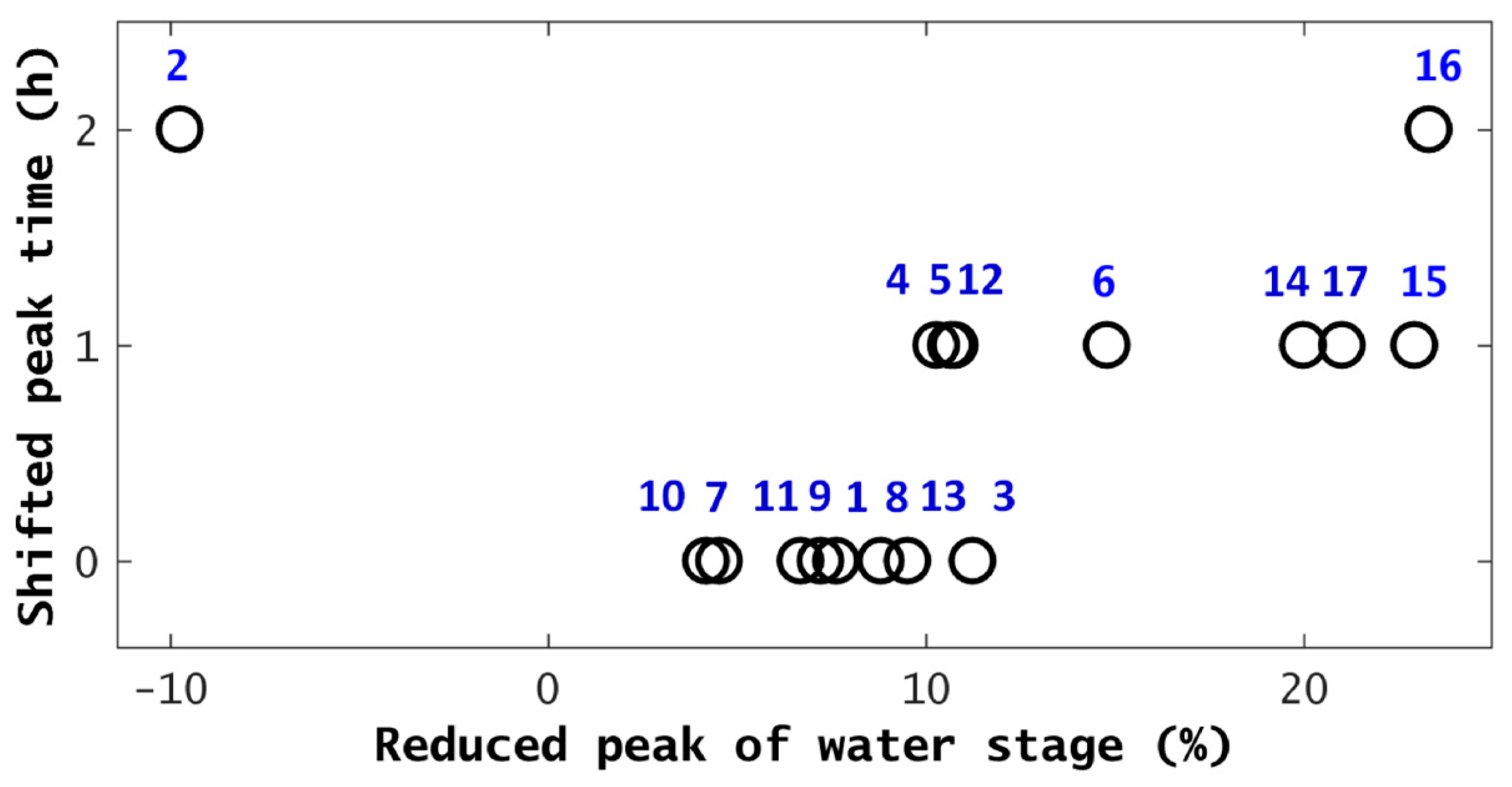
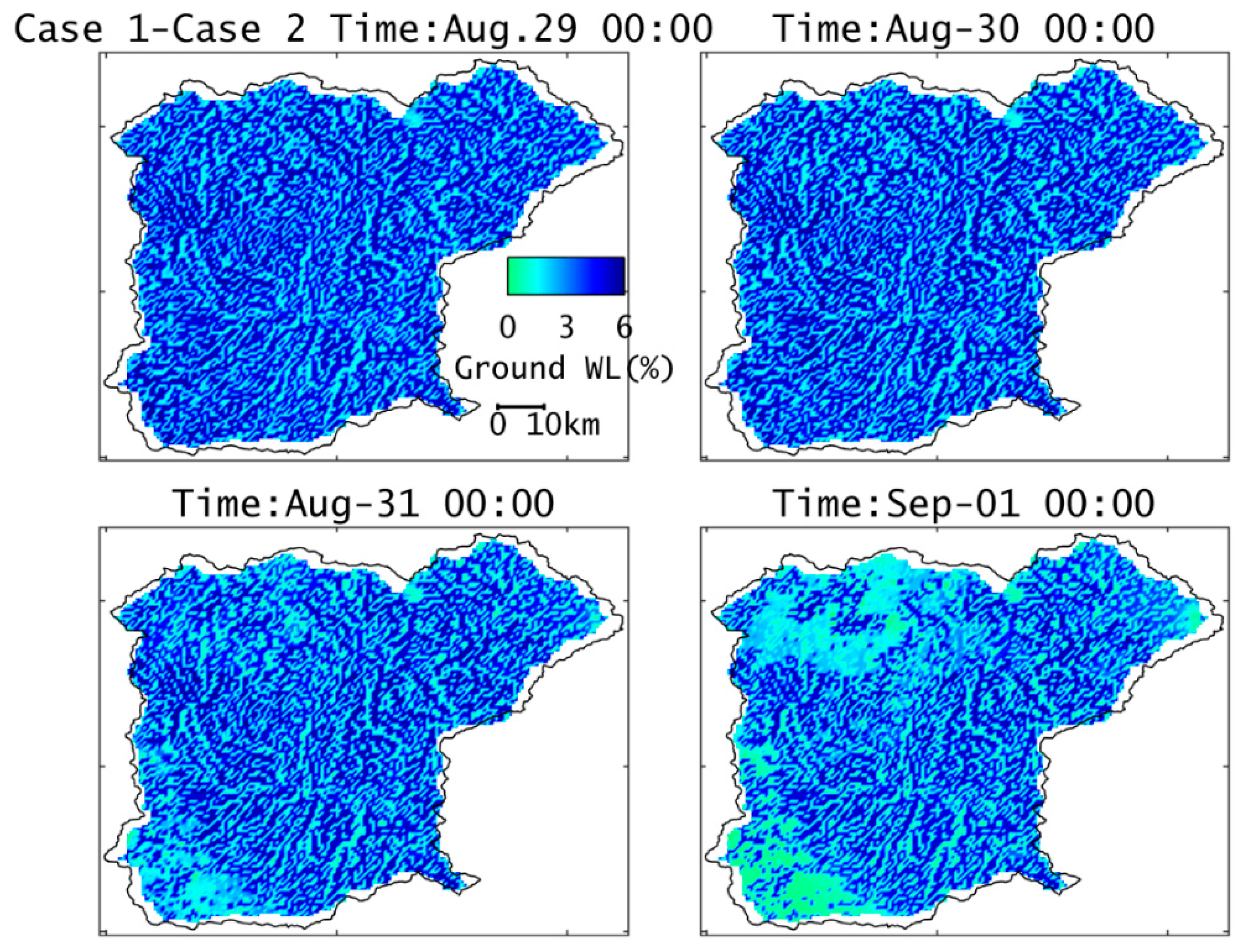
According to a report on the August 2016 disaster [8], saturated soil caused by the preceding three typhoons potentially promoted enormous flood disasters in the west portion of the TR watershed during the approach of the fourth typhoon (i.e., Period II). A simple comparison of the real and artificial simulations associated with soil saturation was performed to quantitatively evaluate the effect of the preceding typhoons on flooding during Period II. The artificial numerical experiment was set up such that no rainfall occurred during the preceding three typhoon attacks (hereafter Period I), but the other meteorological conditions were the same as those of the real simulation (Case 1). Outflows from the flood control dams were provided by the observed discharges at the dam outlets or the estimated discharges, which were computed with dam capacities and inflows when the estimated discharges were higher than the observed ones. We named this numerical examination Case 2. Note that our study focused only on the differences in flood peaks between Case 1 and Case 2. In Figure 6, the difference between both cases shows most water-stage peaks of Case 2 were approximately 4–24% lower than those of Case 1 on 30 August 2016. The peak at Gage 2 (close to Tokachi Dam) was approximately 15% higher than that of Case 1 because the modified flood control at Tokachi Dam was probably inappropriate for Case 2. Figure 6 also shows the peak time when a maximum peak was recorded at each gage during Period II. Half of the peak times in Case 2 were the same as those of Case 1, although several gages recorded up to two-hour peak time delays. For the evaluation of the effect of soil saturation, we gained two quantitative variables: water levels in the surface tank (surface-WL) and the groundwater tank (ground-WL) in the PWRI-DHM outputs. The difference in spatial distributions of surface-WL between Case 1 and Case 2 before Period II was large, with 92% of the spatial distribution of surface WL of Case 1 as the maximum and 60% as the mean over the TR watershed because the surface-WLs of Case 2 were almost zero (Figure 7a). A small rainfall effect for the spin-up time of the simulation still remained and little rainfall by the beginning of the fourth typhoon existed, with a smaller difference in the surface-WLs over the mountain area. The difference became much smaller, reducing from 21% to 1% as the average over the watershed as the amount of precipitation increased (Figure 7b–d). Figure 8 suggests that the spatially distributed ground-WL in Case 2 was slightly reduced, as it represented up to 6% that of Case 1, and the mean was approximately 4% over the TR watershed before and during the early stage of Period II. After the rain event, the ground-WLs of both cases were similar only in the southwest and northwest portions where torrential rain occurred, although the average was still 3% in most areas of the TR watershed.
3.3. Future Flood Situation under Global Warning
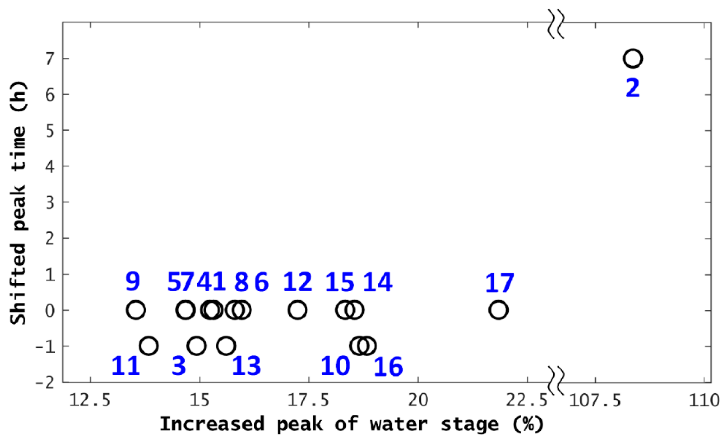
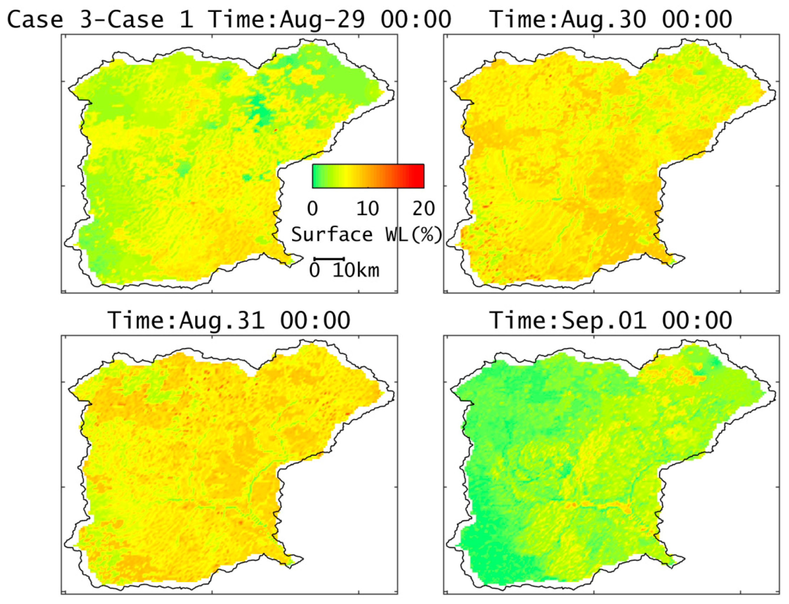
According to the IPCC Fifth Assessment Report (AR5) [14], there is no doubt that global warming will affect future climates over the world and future precipitation will potentially increase in the mid-/high-latitude regions. For Hokkaido, the JMA [25,26] reported that significant climate change will occur between the end of the 20th century (1980–1999) and the end of the 21st century (2075–2095) based on a climate projection (d4PDF [27]) simulated over the Japan area with conditions similar to those of the Representative Concentration Pathway (RCP) 8.5 scenario in the IPCC AR5 [14]. They showed that the precipitation per year will be increased by approximately 10% and the frequencies of climate extremes will increase. For instance, the frequencies of rainfall events with over 100 mm/day and over 30 mm/h will potentially increase by 100% in the North Pacific area in Hokkaido. The above result was obtained using a coarse-resolution regional climate model with a 20-km square grid, which would not be appropriate for the TR watershed because it has less consideration of the local topography in a small watershed. In the TR watershed, future climate outputs from a high-resolution (approximately 5 km) model [28] will be required for a better simulation of future floods. Instead, we conducted a simple numerical examination, assuming the same typhoon conditions as those of the four-typhoon attack in the August 2016 disaster to gain a primitive evaluation for future flood hazards. We set up another numerical examination as Case 3 based on the above implication of future climate. Case 3 had 10% increased precipitation over the TR watershed during the August 2016 disaster as a simple climate condition to obtain preliminary information regarding the effects of future climate conditions. Outflows from the dams were provided using the same method as that used in Case 2 and the other meteorological conditions were the same as those in Case 1. Figure 9 shows that the peak of the water stage at Gage 2 was significantly higher than that of Case 1 (an approximately 140% increase), and a higher delay of the peak time (7 h) during Period II was observed. The large difference was potentially caused by the excess outflow from Tokachi Dam on the main river. The excess outflow beyond the discharge by the flood control in Case 1 occurred owing to a larger amount of inflow from the upstream area when precipitation increased by 10%. Besides the effect of dam operation on flood peak on the main river, the other gages recorded approximately 13–22% increased peaks. In addition, most peak times of Case 3 were shifted forward by an hour and others were the same as those of Case 1 (Figure 9). Figure 10b,c show that the differences in distribution of surface WL between Case 1 and Case 3 were 19% for the maximum distribution and approximately 7% for the average distribution over the TR watershed during Period II. On the contrary, the difference between the ground WLs for Case 1 and Case 3 was less than 1%.
4. Discussion
Our results provide two discussion points: the impact of the preceding three typhoons and future flood simulation based on the hydrological model appropriately validated with the observed data during the August 2016 disaster. The preceding three typhoons brought heavy rainfall to the TR watershed during Period I. The amount of the accumulated precipitation was approximately 60% of the total accumulated precipitation (Figure 2). On the other hand, the accumulated precipitation was approximately 35% during Period II when higher flood peaks severely damaged the west portion of the TR watershed. The numerical experiment that did not consider the impact of the preceding three typhoons revealed that flood peaks during Period II reduced 4–24% for most gage stations (except for Gage 2) and half of the peak times were shifted backward by two hours (Figure 6). In particular, the flood peaks in the N-tributaries (Gages 14–17) were over 15% lower than those of Case 1 because the precipitation during Period I more greatly affected these flood peaks than the later precipitation during Period II. The largely reduced discharges at the N-tributaries resulted in a relatively large reduction (10–15%) in flood peaks on the main river (gage stations 3–6). A general reason for the peak reduction and peak-time delay was the difference in the degree of soil saturation in the surface layer between Case 1 and Case 2. In fact, the surface-WL distribution in Case 2 eventually reached that of Case 1 (Figure 7) and the water capacity of the soil was almost zero for Case 2 before Period II (Figure 7a). However, the soil in the surface layer was suddenly saturated during Period II due to the much greater precipitation that occurred in this period, which resulted in the soil achieving full water capacity within a short time period. These results imply that the soil in the surface layer was already saturated late into Period II. Therefore, the impact of the preceding three typhoons was significant until the early stage of Period II, and then was weak after the middle stage of Period II because the impact of the heavy rainfall during Period II was suddenly superior to the residual impact of the Period I rainfall. In the groundwater layer, a comparison of both cases did not show significant changes in the distributions of the ground WLs (Figure 8). In short, the rainfall event during Period II, especially in the west portion of the TR watershed, can be characterized by a much shorter and much heavier event than past rainfall events [8]. The event brought such heavy rainfall that soil in the area was unable to retain the water from the event for a longer period of time.
As mentioned in the IPCC reports [5,6,14], the number of typhoons that strike the mid-latitude regions may increase in the future. A preliminary simulation was run with a simple assumption and coarse climate information, as a database with refined and high-resolution climate projections has not yet been prepared. A comparison between Case 1 and Case 3 on flood peaks and peak times showed most gage stations observed approximately 13–22% increased flood peaks for Case 3 during Period II (Figure 9). These increased peaks potentially corresponded to a 10% increased precipitation over the TR watershed. The variations in the increased peaks might be caused by the distribution of the surface WL (Figure 10). The largely increased surface-WL was distributed in the areas close to the river mouth, which suggested that the soil had some room to retain the excess water from heavier rainfall in the southern TR watershed. Flood peak times were shifted forward by an hour (Figure 9) because the excess flow from the considerable amount of earlier precipitation during Period II moved to the river courses. In contrast, there was only a small difference in ground WLs between Case 1 and Case 3 in the groundwater layer. This result suggests that extra soil water capacity hardly existed in the groundwater layer during the heavy rainfall event.
In addition, Figure 6 and Figure 9 showed the flood peaks at Gage 2 for two numerical experiments (Case 2 and Case 3) largely increased during Period II likely because of poorly adapted flood control during the heavy rainfall event. In particular, the flood peak at Gage 2 in Case 3 increased considerably. Gage 2 is located near the Tokachi Dam, which performed outflow discharge with adaptive flood control during Periods I and II. Adaptive flood control in the dam was one of the important factors that reduced flood risk during the August 2016 disaster. In particular, Tokachi Dam successfully reduced flood risk in the downstream areas along the main river during Period II by performing a prior discharge before the fourth typhoon struck. This type of adaptive flood control is sometimes employed because of water capacity management in a dam [29] and as a further development, should be incorporated with a climate model [30]. However, the result of Case 3 (Figure 9) implies that the flood control of Case 1 at Tokachi Dam may not work for a future flood.
5. Conclusions
With quantitative variables such as flood peak and soil saturation we assessed the impact of multiple typhoons on flood disasters that may occur in the mid-latitude regions in the near future. After validating the distributed hydrological model in the TR watershed during the multiple floods (Case 1) caused by a preceding heavy rainfall event (Period I) and a subsequent heavier rainfall event (Period II), we ran two numerical experiments that assumed the preceding rainfall event did not have any impact on the area (Case 2) and considered a pseudo future climate (Case 3). The findings of this study are as follows.
- The water stage peaks for most gage stations during Period II were reduced by 4–24% when the impact of the preceding typhoons was not considered (Case 2) because the water capacity of the soil was not full over the watershed before the fourth typhoon.
- Most future peaks (Case 3) were 13–22% higher than those in Case 1 under the effect of a 10% higher precipitation because the maximum difference between the water capacities of the soil in Case 1 and Case 3 was 10–20%.
- The peaks and peak times at Gage 2 in Case 2 and Case 3 were significantly different from those of the other stations. These results suggest that adaptive flood control corresponding to the inflow in Tokachi Dam as well as the dam capacity were important factors that reduced flood risk.
In future work, high-resolution climate projections [28] will be implemented in the distributed hydrological model validated in this study.
Author Contributions
N.K., H.K. and I.K. contributed to the design and implementation of the research. N.K. performed the simulations and the data analyses. All authors discussed the results and contributed to the final manuscript.
Acknowledgments
This study was supported by the Ministry of Education, Culture, Sports, Science and Technology of Japan under the framework of the TOUGOU Program. We would also like to thank the anonymous reviewers for their helpful suggestions.
Conflicts of Interest
The authors declare no conflicts of interest.
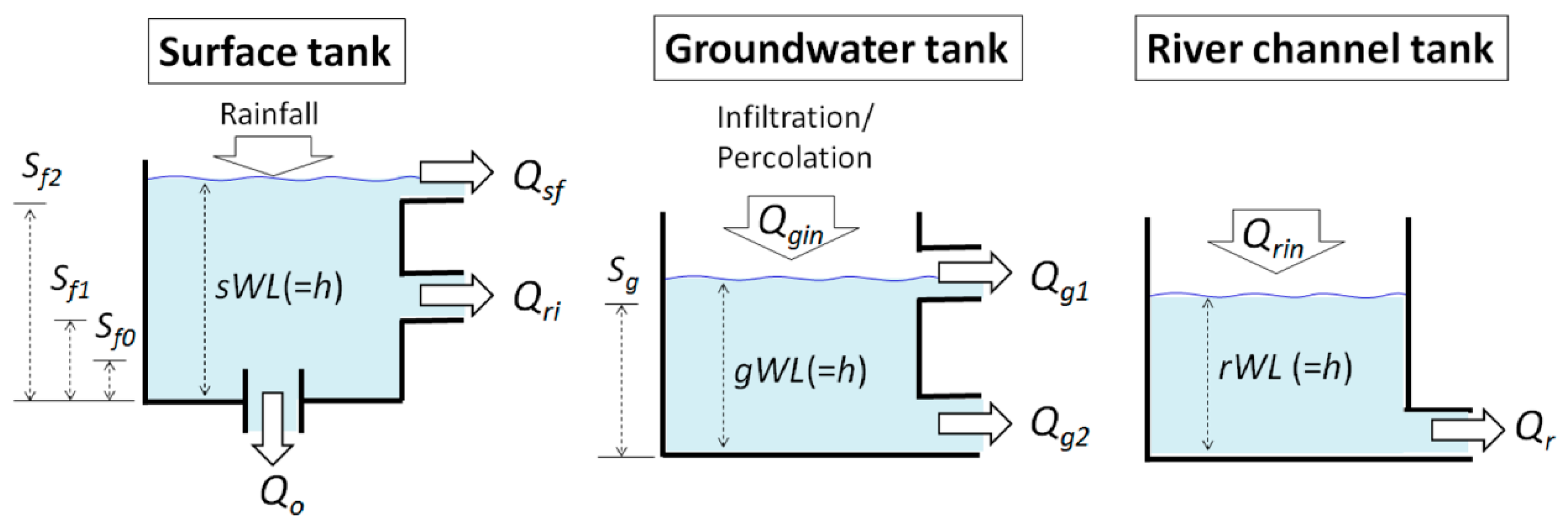
Appendix A
The PWRI-DHM employs the tank model, which has surface, groundwater, and river tanks, and the concept is shown in Figure A1. From the amount of precipitation, the surface tank provides the surface flow () (cms), rapid intermediate outflow () (cms), and infiltration flow () (cms) to the underground. The surface flow is given by
where is the height of stored water (m), is the height (m) where appears, is the roughness coefficient (s/m1/3) of the surface tank, is the length of cell (°), and is the gradient of slope. The intermediate and infiltration outflows are proportional to the water stored in soil. They are respectively given by
where is the height (m) where appears, is the coefficient for intermediate flow, is the infiltration capacity (m/s), and is the area of cell (m2), and
where is the height (m) where appears. becomes the inflow of the groundwater tank. The relationships between temporal deviation of the height, flows, and rainfall in the surface tank are provided by
where is the rainfall (m) and is the actual evapotranspiration (m), computed by the Penman–Monteith equation. With the percolation inflow ( = ) (cms) through the surface tank, the groundwater tank provides two outlet flows: unconfined groundwater flow () (cms), which is proportional to the second power of the water stored in soil, and confined groundwater flow () (cms), which is proportional to the water stored in soil. and are respectively given by
where is the height (m) where appears, and (1/(ms)1/2) and (1/s) are the coefficients of slow intermediate outflow and base outflow respectively. The relationship between temporal deviation of the height and in/outflows in the groundwater tank is given by
For the river tank, the flow of the river () (cms) is assumed to be governed by Manning’s formula and is provided by
where is the breadth of the river (m), is the roughness coefficient of the channel (s/m1/3) and is the gradient of the channel. The relation between temporal deviation of the height and in/outflows is described as
where is the inflow (cms) through the surface tanks and groundwater tanks, and is the length of river (m). For the setup of the hydrological parameters at each tank, all cells are classified to several parameter groups based upon the distance from the upper stream, land-use, and soil-type information. Each group has its own values, shown as the default values in Table A1, which were calibrated for the East Asia watersheds. Further information is available on the ICHARM website [16].

Table A1.
Default values for the parameters of each tank model.
| Surface Tank | Groundwater Tank | River Tank | |
|---|---|---|---|
| Infiltration capacity (, m/s) | 1 × 10⁻⁸–5 × 10⁻⁶ | ‒ | ‒ |
| Maximum height (, m) | 0.001–0.1 | ‒ | ‒ |
| Height where intermediate outflow appears (, m) | 0.0005–0.01 | ‒ | ‒ |
| Height where infiltration appears (, m) | 0.0001–0.005 | ‒ | ‒ |
| Surface roughness coefficient (, s/m1/3) | 0.1–2.0 | ‒ | ‒ |
| Coefficient of intermediate outflow () | 0.5–0.9 | ‒ | ‒ |
| Coefficient of slow intermediate outflow (, 1/(ms)1/2) | ‒ | 0.011 | ‒ |
| Coefficient of base outflow (, 1/s) | ‒ | 3.5 × 10⁻⁸ | ‒ |
| Height where slow intermediate outflow appears (, m) | ‒ | 2.0 | ‒ |
| Manning roughness coefficient of river (, s/m1/3) | ‒ | ‒ | 0.035 |
Note that the ranges of some parameters depend on the classification of each tank’s characteristics.
Figure A1.
Schematic conception of three-tank model in the Public Works Research Institute-Distributed Hydrological Model (PWRI-DHM).
Figure A1.
Schematic conception of three-tank model in the Public Works Research Institute-Distributed Hydrological Model (PWRI-DHM).

References
- Japan Meteorological Agency (JMA)—The Regional Specialized Meteorological Center (RSMC) Tokyo—Typhoon Center. Available online: http://www.jma.go.jp/jma/jma-eng/jma-center/rsmc-hp-pub-eg/RSMC_HP.htm (accessed on 1 April 2018).
- Myeong, S.; Hong, H.J. Developing flood vulnerability map for North Korea. In Proceedings of the American Society for Photogrammetry and Remote Sensing Annual Conference, Baltimore, MD, USA, 26–28 March 2009; pp. 9–13. [Google Scholar]
- Takano, K.T.; Nakagawa, K.; Aiba, M.; Oguro, M.; Morimoto, J.; Furukawa, Y.; Mishima, Y.; Ogawa, K.; Ito, R.; Takemi, T. Projection of impacts of climate change on windthrows and evaluation of potential adaptation measures in forest management: A case study from empirical modelling of windthrows in Hokkaido, Japan, by Typhoon Songda (2004). Hydrol. Res. Lett. 2016, 10, 132–138. [Google Scholar] [CrossRef] [Green Version]
- Kanada, S.; Tsuboki, K.; Aiki, H.; Tsujino, S.; Takayabu, I. Future enhancement of heavy rainfall events associated with a typhoon in the midlatitude regions. SOLA 2017, 13, 246–251. [Google Scholar] [CrossRef]
- Intergovernmental Panel on Climate Change (IPCC). Managing the Risks of Extreme Events and Disasters to Advance Climate Change Adaptation; A Special Report of Working Groups I and II of the IPCC; Field, C.B., Barros, V., Stocker, T.F., Qin, D., Dokken, D.J., Ebi, K.L., Mastrandrea, M.D., Mach, K.J., Plattner, G.-K., Allen, S.K., et al., Eds.; Cambridge University Press: Cambridge, UK; New York, NY, USA, 2012. [Google Scholar]
- Intergovernmental Panel on Climate Change (IPCC). Contribution of Working Group II to the Fourth Assessment Report of the IPCC; Parry, M.L., Canziani, O.F., Palutikof, J.P., van der Linden, P.J., Hanson, C.E., Eds.; Cambridge University Press: Cambridge, UK; New York, NY, USA, 2007. [Google Scholar]
- Hoshino, G.; Yamada, T.J. Impact Assessment of Climate Change on Precipitation over a Watershed in Hokkaido, Proceedings of the 2017 Annual Conference of the Japan Society of Hydrology and Water Resources Forum. Title Was Translated by N. Kimura. Available online: https://doi.org/10.11520/jshwr.30.0_12 (accessed on 1 April 2018). (In Japanese).
- Japan Society of Civil Engineers (JSCE). Onsite Field Investigation Team, Site-Investigation Report for the Hokkaido Heavy Rain Disasters in August 2016; Title was translated by N. Kimura; JSCE Report; JSCE: Tokyo, Japan, 2017. (In Japanese) [Google Scholar]
- Ministry of Land, Infrastructure, Transport, and Tourism in Japan (MLIT Japan). Hydrology and Water Quality Database. Available online: http://www1.river.go.jp/ (accessed on 1 April 2018).
- MLIT Japan. Future Countermeasures for Flood Controls with the Consideration of the Hokkaido Heavy-Rain Disaster in August 2016—Supplementary Material. Title Was Translated by N. Kimura. Available online: https://www.hkd.mlit.go.jp/ky/kn/kawa_kei/ud49g7000000f0l0-att/splaat000000hdsv.pdf (accessed on 1 April 2018). (In Japanese)
- Osanai, N.; Kasai, M.; Hayashi, S.I.; Katsura, S.Y.; Furuichi, T.; Igura, M.; Kosaka, M.; Fujinami, T.; Mizugaki, S.; Abe, T.; et al. Sediment discharge in the Tokachi region, Hokkaido, caused by Typhoon No. 10 (Lionrock), 2016. Jpn. Soc. Eros. Control Eng. 2017, 69, 80–91. (In Japanese) [Google Scholar]
- Nakatsugawa, M. Survey on factors of geotechnical disaster in Hidaka region due to Typhoon No. 10 in 2016. Mem. Muroran Inst. Technol. 2018, 67, 3–8. (In Japanese) [Google Scholar]
- Hokkaido Regional Development Bureau in MLIT Japan. Obihiro Office Website. Available online: https://www.hkd.mlit.go.jp/ob/obihiro_kasen/index.html (accessed on 1 April 2018).
- Intergovernmental Panel on Climate Change (IPCC). Climate Change 2013: The Physical Science Basis. Contribution of Working Group I to the Fifth Assessment Report of the IPCC; Stocker, T.F., Qin, D., Plattner, G.-K., Tignor, M., Allen, S.K., Boschung, J., Nauels, A., Xia, Y., Bex, V., Midgley, P.M., Eds.; Cambridge University Press: Cambridge, UK; New York, NY, USA, 2013. [Google Scholar]
- Fukami, K.; Sugiura, Y.; Magome, J.; Kawakami, T. Integrated flood analysis system (IFAS Ver. 1.2)—User’s manual. Jpn. PWRI-tech. Note 2009, 4148, 223. [Google Scholar]
- International Centre for Water Hazard and Risk Management (ICHARM). IFAS Flood Forecasting System Using Global Satellite Rainfall. Available online: http://www.icharm.pwri.go.jp/research/ifas/ (accessed on 1 April 2018).
- Aziz, A.; Tanaka, S. Regional parameterization and applicability of Integrated Flood Analysis System (IFAS) for flood forecasting of upper-middle Indus River. Pak. J. Meteorol. 2011, 8, 21–38. [Google Scholar]
- Liu, T.; Tsuda, M.; Iwami, Y. A study on flood forecasting in the upper Indus basin considering snow and glacier meltwater. J. Disaster Res. 2017, 12, 793–805. [Google Scholar] [CrossRef]
- Yoshino, F.; Yoshitani, J.; Sugiura, M. A Conceptual Distributed Model for Large-Scale Mountainous Basins. In Hydrology of Mountainous Regions, I—Hydrological Measurements; The Water Cycle; Lang, H., Musy, A., Eds.; IAHS Publisher: Lausanne, Switzerland, 1990; pp. 685–692. [Google Scholar]
- HydroSHEDS. Available online: www.hydrosheds.org (accessed on 1 April 2018).
- Global Land Cover Characterization (GLCC). Available online: https://lta.cr.usgs.gov/GLCC (accessed on 1 April 2018).
- JMA. Past Meteorological Data. Available online: http://www.data.jma.go.jp/gmd/risk/obsdl/index.php (accessed on 1 April 2018).
- Kimura, N.; Chiang, S.; Wei, H.P.; Su, Y.F.; Chu, J.L.; Cheng, C.T.; Liou, J.J.; Chen, Y.M.; Lin, L.Y. Hydrological flood simulation to Tsengwen reservoir watershed under global climate change with 20 km mesh Meteorological Research Institute atmospheric general circulation model (MRI-AGCM). Terr. Atmos. Ocean. Sci. 2014, 25, 449–461. [Google Scholar] [CrossRef]
- Nash, J.E.; Sutcliffe, J.V. River flow forecasting through conceptual models part I—A discussion of principles. J. Hydrol. 1970, 10, 282–290. [Google Scholar] [CrossRef]
- JMA. Global Warming Forecast Report; Title Was Translated by N. Kimura; JMA: Tokyo, Japan, 2013; Volume 8. (In Japanese)
- JMA Sapporo Branch. Climate Change in Hokkaido—120-Year Observations and Forecasts, 2nd ed.; Title Was Translated by N. Kimura; JMA Sapporo branch: Sapporo, Japan, 2017. (In Japanese)
- Database for Policy Decision-Making for Future Climate Change (d4PDF). Available online: http://www.miroc-gcm.jp/~pub/d4PDF/index_en.html (accessed on 1 April 2018).
- JMA. Global Warming Forecast Report; Title Was Translated by N. Kimura; JMA: Tokyo, Japan, 2017; Volume 9. (In Japanese)
- Asia Pacific Adaptation Network. Risk Management in Dam Operation: A Approaches to Improve Flood Control Capabilities of Existing Dams. Available online: http://www.asiapacificadapt.net/adaptation-technologies/database/risk-management-dam-operation-aapproaches-improve-flood-control (accessed on 1 April 2018).
- Mitsuishi, S.; Ozeki, T.; Sumi, T. Applicability of a New Flood Control Method Utilizing Rainfall Prediction by WRF. J. Jpn. Soc. Hydrol. Water Resour. 2011, 24, 110–120. (In Japanese) [Google Scholar] [CrossRef] [Green Version]
Figure 1.
Hokkaido map and the elevation map of the Tokachi River (TR) watershed. Blue lines show the rivers; circles, diamonds, and squares show the water stage gages on the main river and the southern and northern tributaries of the main river, respectively. The yellow inverted triangles indicate dams.

Figure 2.
Accumulated distributions of the precipitation from 16 August to 5 September, 16–24 August (Period I), and 29–31 August (Period II), 2016. The spatial distributions were determined by using the ordinary kriging method. Symbols × and ∗ indicate the locations of the Naitai and Nukabira-Gensenkyo rain gage stations respectively, which recorded the large amounts of precipitation that were used as representative data.

Figure 3.
Water-stage comparison between simulation (red line) and observation (black circle) in the main river from the upstream to the downstream with mean rainfall (blue box) over an upstream area from each gage station: (a) Nishibetsu; (b) Kyohei Bridge; (c) Memurobuto; (d) Obihiro; (e) Tokachichuoh Bridge; and (f) Moiwa.

Figure 4.
Comparison between simulated and observed water-stages in S-tributaries with mean rainfall over an upstream area from each gage station: (a) Bisei Bridge; (b) Higashisanjyo; (c) Rrutanjyoryu; (d) Dainiohkawa Bridge; (e) Totta Bridge; and (f) Yamuwakka.
Figure 4.
Comparison between simulated and observed water-stages in S-tributaries with mean rainfall over an upstream area from each gage station: (a) Bisei Bridge; (b) Higashisanjyo; (c) Rrutanjyoryu; (d) Dainiohkawa Bridge; (e) Totta Bridge; and (f) Yamuwakka.

Figure 5.
Comparison between simulated and observed water-stages in N-tributaries with mean rainfall over an upstream area from each gage station: (a) Otofuke; (b) Asahi Bridge; (c) Azuma Bridge; (d) Toshibetsu; and (e) Todaiichigo Bridge.
Figure 5.
Comparison between simulated and observed water-stages in N-tributaries with mean rainfall over an upstream area from each gage station: (a) Otofuke; (b) Asahi Bridge; (c) Azuma Bridge; (d) Toshibetsu; and (e) Todaiichigo Bridge.

Figure 6.
Differences in water stage peaks (SP) between the real case (Case 1) and the ideal case (Case 2) during Period II, showing a shifted peak time from the peak time of Case 1 (h) vs. reduced peak (%) of the water stage. The reduced peak was calculated using the formula (SPCase1 − SPCase2)/SPCase1 × 100 (%).

Figure 7.
Differences in water levels in the surface tank (surface-WLs) between Case 1 and Case 2 before, during, and after the approach of the fourth typhoon (Period II) over the TR watershed. Reduction in the surface-WL by the formula (surfaceWLCase1 − surfaceWLCase2)/surfaceWLCase1 × 100 (%).
Figure 7.
Differences in water levels in the surface tank (surface-WLs) between Case 1 and Case 2 before, during, and after the approach of the fourth typhoon (Period II) over the TR watershed. Reduction in the surface-WL by the formula (surfaceWLCase1 − surfaceWLCase2)/surfaceWLCase1 × 100 (%).

Figure 8.
Differences in water levels in the groundwater tank (ground-WLs) between Case 1 and Case 2 before, during, and after the Period II over the TR watershed. Reduction in the ground-WL was calculated by the formula (groundWLCase1 − groundWLCase2)/groundWLCase1 × 100 (%).
Figure 8.
Differences in water levels in the groundwater tank (ground-WLs) between Case 1 and Case 2 before, during, and after the Period II over the TR watershed. Reduction in the ground-WL was calculated by the formula (groundWLCase1 − groundWLCase2)/groundWLCase1 × 100 (%).

Figure 9.
Differences in water stage peaks (SP) between Case 1 and Case 3 (future simulation), showing increased peak (%) vs. shifted peak time from the peak time of Case 1 (h). The increased peak was calculated using the formula (SPCase3 − SPCase1)/SPCase1 × 100 (%).
Figure 9.
Differences in water stage peaks (SP) between Case 1 and Case 3 (future simulation), showing increased peak (%) vs. shifted peak time from the peak time of Case 1 (h). The increased peak was calculated using the formula (SPCase3 − SPCase1)/SPCase1 × 100 (%).

Figure 10.
Differences in surface WL between Case 1 and Case 3 (future simulation) before, during, and after the approach of the fourth typhoon over the TR watershed. The increase in the surface-WL was calculated by the formula (surfaceWLCase3 − surfaceWLCase1)/surfaceWLCase1 × 100 (%).
Figure 10.
Differences in surface WL between Case 1 and Case 3 (future simulation) before, during, and after the approach of the fourth typhoon over the TR watershed. The increase in the surface-WL was calculated by the formula (surfaceWLCase3 − surfaceWLCase1)/surfaceWLCase1 × 100 (%).

Table 1.
Typhoon characteristics.
| Asian Typhoon Name | Date and Time of Landing/Approach (August 2016) 1 | Minimum Central Pressure (hPa) 1 | Maximum Wind Speed (m/s) 1 | Accumulated Precipitation (mm) 2 |
|---|---|---|---|---|
| Chanthu | 17, 17:00 | 980 | 30 | 197 (48 h) |
| Kompasu | 21, 23:00 | 1002 | 18 | 183 (48 h) |
| Mindulle | 23, 06:00 | 992 | 25 | 103 (24 h) |
| Lionrock | 30, 17:00 | 965 | 35 | 352 (72 h) |
Table 2.
Flood control dam information.
| Dam Name | Location | Catchment Area (km2) | Capacity (million m3) | Length (m) | Height (m) | Surface Area (km2) |
|---|---|---|---|---|---|---|
| Tokachi | 43.240° N, 142.939° E | 592.0 | 112.0 | 443.0 | 84.3 | 4.2 |
| Satsunai River | 42.588° N, 142.923° E | 117.7 | 54.0 | 300.0 | 114.0 | 1.7 |
Note that these data were obtained from the website of the Obihiro office of the Hokkaido Regional Development Bureau of the Ministry of Land, Infrastructure, Transport, and Tourism of Japan (MLIT) Japan [13].
Table 3.
Validation of model simulation at water stage gages. NS: Nash–Sutcliffe model efficiency coefficient; Rp: reproducibility; MAE: mean absolute error.
Table 3.
Validation of model simulation at water stage gages. NS: Nash–Sutcliffe model efficiency coefficient; Rp: reproducibility; MAE: mean absolute error.
| Number | Station Name | Location | Rp | NS | MAE (m) | rMAE * (%) | Remarks |
|---|---|---|---|---|---|---|---|
| 1 | Nishibetsu | 43.323° N, 142.943° E (Main stream) | 0.74 | 0.78 | 0.27 | 8.6 | Gage stopped after 23 August, 9:00. |
| 2 | Kyohei Bridge | 43.068° N, 142.926° E (Main stream) | 0.75 | 0.48 | 0.51 | 32.3 | |
| 3 | Memurobuto | 42.931° N, 143.047° E (Main stream) | 0.73 | 0.71 | 0.19 | 4.1 | |
| 4 | Obihiro | 42.934° N, 143.203° E (Main stream) | 0.77 | 0.74 | 0.47 | 7.4 | Near Obihiro City |
| 5 | Tokachichuoh Bridge | 42.927° N, 143.291° E (Main stream) | 0.76 | 0.78 | 0.35 | 5.2 | |
| 6 | Moiwa | 42.808° N, 143.512° E (Main stream) | 0. 63 | 0.41 | 1.23 | 12.0 | |
| 7 | Bisei Bridge | 42.923° N, 143.066° E (S-tributaries) | 0.63 | 0.68 | 0.24 | 8.53 | |
| 8 | Higashisanjyo | 42.933° N, 143.209° E (S-tributaries) | 0.46 | 0.57 | 0.30 | 9.1 | |
| 9 | Rrutanjyoryu | 42.611° N, 142.870° E (S-tributaries) | 0.75 | 0.83 | 0.13 | 5.6 | Gage stopped after 30 August, 20:00. |
| 10 | Dainiohkawa Bridge | 42.798° N, 143.157° E (S-tributaries) | 0.75 | 0.84 | 0.24 | 6.2 | |
| 11 | Totta Bridge | 42.699° N, 143.058° E (S-tributaries) | 0.73 | 0.73 | 0.17 | 8.0 | Gage stopped after 31 August, 2:00. |
| 12 | Yamuwakka | 42.910° N, 143.356° E (S-tributaries) | 0.53 | 0.48 | 0.47 | 7.0 | |
| 13 | Otofuke | 43.008° N, 143.200° E (N-tributaries) | 0.64 | 0.68 | 0.2 | 6.3 | |
| 14 | Asahi Bridge | 42.947° N, 143.270° E (N-tributaries) | 0.66 | 0.64 | 0.16 | 5.7 | |
| 15 | Azuma Bridge | 43.094° N, 143.516° E (N-tributaries) | 0.83 | 0.89 | 0.20 | 5.5 | |
| 16 | Toshibetsu | 42.931° N, 143.443° E (N-tributaries) | 0.69 | 0.74 | 0.45 | 7.2 | |
| 17 | Todaiichigo Bridge | 42.920° N, 143.476° E (N-tributaries) | 0.49 | 0.26 | 0.45 | 9.6 |
* rMAE is defined by MAE/total variation in water stage ×100.
© 2018 by the authors. Licensee MDPI, Basel, Switzerland. This article is an open access article distributed under the terms and conditions of the Creative Commons Attribution (CC BY) license (http://creativecommons.org/licenses/by/4.0/).
Share and Cite
MDPI and ACS Style
Kimura, N.; Kiri, H.; Kitagawa, I. The Impact of Multiple Typhoons on Severe Floods in the Mid-Latitude Region (Hokkaido). Water 2018, 10, 843. https://doi.org/10.3390/w10070843
AMA Style
Kimura N, Kiri H, Kitagawa I. The Impact of Multiple Typhoons on Severe Floods in the Mid-Latitude Region (Hokkaido). Water. 2018; 10(7):843. https://doi.org/10.3390/w10070843
Chicago/Turabian StyleKimura, Nobuaki, Hirohide Kiri, and Iwao Kitagawa. 2018. "The Impact of Multiple Typhoons on Severe Floods in the Mid-Latitude Region (Hokkaido)" Water 10, no. 7: 843. https://doi.org/10.3390/w10070843
Note that from the first issue of 2016, this journal uses article numbers instead of page numbers. See further details here.