Monitoring Biological and Chemical Trends in Temperate Still Waters Using Citizen Science


1
Earthwatch Institute (Europe), Mayfield House, 256 Banbury Road, Summertown, Oxford OX2 7DE, UK
2
College of Liberal Arts (CoLA), Bath Spa University, Newton St. Loe, Bath BA2 9BN, UK
3
School of Geography and the Environment, University of Oxford, South Parks Road, Oxford OX1 3QY, UK
4
Department of Biotechnology, Chemistry and Pharmacy, University of Siena, Via Aldo Moro 2, 53100 Siena, Italy
*
Author to whom correspondence should be addressed.
Water 2018, 10(7), 839; https://doi.org/10.3390/w10070839
Submission received: 11 April 2018
/
Revised: 28 May 2018
/
Accepted: 14 June 2018
/
Published: 25 June 2018
(This article belongs to the Section Water Quality and Contamination)
Abstract
:The involvement of volunteers in the monitoring of the environment holds great potential to gather information on a wider temporal and spatial scale than is currently possible. However, the mass involvement of citizens in monitoring freshwater health is a relatively new field and subject to uncertainty. Here, we examine 1192 samples collected across 46 temperate ponds (<2 ha) and 29 temperate lakes (>2 ha) by 120 volunteers trained through the FreshWater Watch citizen science programme to consider if the approach is able to (a) identify well established patterns in water quality and biological indicators (i.e., fish), and (b) provide a potentially useful basis for the identification of pollution sources in urban or peri-urban landscapes. Seasonal patterns observed agreed well with established principles of nutrient dynamics, algal bloom seasonality, and broad biological trends between ponds and lakes. Further, observational data collected by the volunteers suggested plausible links between the presence of residential discharge and water level fluctuation and significant increases in algal bloom observations between peri-urban and urban sites. We suggest that citizen science can have a role to play in complementing regulatory monitoring efforts and that local citizens should be empowered to become stewards of their local freshwater resources.
1. Introduction
The number and importance of ponds and small lakes far outweighs the attention given to their study and management [1]. Small waterbodies (<2 ha) contain a disproportionate amount of freshwater biodiversity [2,3] and provide ecosystem services with important local and global benefits [4]. Yet, the conventional conservation and monitoring priorities have been focused on large lakes and reservoirs. For example, the EU Water Framework Directive 2000/16/EC excludes the majority of small water bodies [5]. This dilemma presents an opportunity for the collection of ecological information regarding these local water bodies using non-conventional monitoring approaches [6]. One such rapidly emerging approach is citizen science, the participation of ordinary members of the public in scientific research [7,8]. However its effectiveness remains largely untested [9].
Seasonal fluctuations in nutrient status and algal growth patterns in temperate lakes are relatively well understood thanks to long term lake monitoring (e.g., North Temperate Lakes) and shallow lakes research [10]. In contrast to deep, stratified lakes, the intense sediment–water interface in shallow ponds and lakes ensures a rapid return of most sediment material into the water column [11]. In addition, the relatively high sediment temperatures in summer lead to an increase in mineralization rates, and consequently to an increased release of phosphorous from the sediment into its soluble form [12]. Thus, a summer peak in phosphate (P-PO4) concentrations is observed. By contrast, soluble nitrate peak concentrations (N-NO3) typically occur during the winter months after a period of plant senescence, with minima in early summer following aquatic vegetation growth. Algal growth patterns reflect nutrient availability in the water column. In the first instance, internally loaded phosphate can result in algal blooms during early summer [13]. Secondarily, an autumn bloom may be observed under suitable temperature and light conditions in response to nutrients released from decaying plant material [11]. In addition, fish presence is increasingly likely in larger water bodies [14,15]. These same patterns should be easily identifiable through a citizen science approach.
Shallow lakes are often considered more susceptible to local and global environmental change than deeper water bodies, because of their limited volume and depth [10] such that the effect of urbanization upon them could be profound and greatly interfere with natural processes [16], as in urban streams [17]. By contrast, the typically reduced catchment area of ponds allows for the possibility that these ecosystems can avoid some of the impacts that plague water bodies with large catchments [18,19]. Previously cited effects of urbanization upon the water quality of still waters are nutrient concentration increases [19,20], greater frequency of algal blooms [21] as well as increased trace metal concentrations and the presence of invasive species [16]. However, it is not clear whether these effects hold true for smaller still waters such as ponds (<2 ha [22]) as they do lakes.
In addition to supporting scientific research and environmental monitoring, citizen science also provides potential benefits associated with environmental awareness and education and advocacy on environmental issues [23,24]. FreshWater Watch (FWW) is the first global citizen science research project studying freshwater ecosystem dynamics. Within FWW, 30 local projects in more than 20 countries have been established; generating information on more than 1500 waterbodies, many of which are small ponds and lakes, in both temperate and tropical regions that hold local cultural importance (https://freshwaterwatch.thewaterhub.org/). Through the participation of citizen scientists, researchers have been able to gather data over a large spatial and temporal scale [25]. Using data collection at such resolution, it should be possible to explore if expected seasonal dynamics, reported for large waterbodies, are also the dominant trends in smaller water bodies and if drivers such as urbanization or an elevated surface to volume ratio lead to modified seasonal dynamics.
This study represents a first attempt to compare seasonal trends between lake and ponds using citizen science gathered data. We explore the effect of increasing urbanization on the seasonal chemical and biological conditions of ponds and lakes. We use a dataset of 1192 measurements from 75 temperate still waters in three continents. Field data were gathered by trained citizen scientists and combined with freely available, global datasets. Using this data, the following hypotheses were tested:
- Seasonal fluctuations would be detected in four parameters indicative of water quality; nitrate (N-NO3), phosphate (P-PO4), turbidity (NTU), and frequency of algal blooms.
- The presence of fish will be recorded with greater frequency in lakes (>2 ha) than in ponds (<2 ha).
- The effect of urbanization would be more pronounced in lakes than in ponds.
Finally, we applied the field data to highlight any potential drivers of those water chemistry factors that exhibited a clear difference between urban and peri-urban sites.
2. Materials and Methods
2.1. Study Area
1192 samples were used in the present study taken from 75 ponds (see Supplementary Material Table S1) and lakes (mean 47,956 m2, min. 10 m2, max. 444,745 m2) within temperate broadleaf, coniferous, and mixed forests, as defined within terrestrial ecosystems of the world [26], across the continents of Europe, North America, and Oceania (Figure 1). Sites were located in urban and peri-urban areas as part of the FWW programme and are mostly manmade having been built for a range of purposes including recreation (e.g., fishing) and infrastructure (e.g., stormwater lagoons). All data are uploaded and open access (freshwaterwatch.thewaterhub.org/content/data-map).
Data were collected by 120 trained citizen scientists (from >8000 total trained) using standardized methods. Quality control against standard methods was conducted with approximately 10% of the samples [27,28]. Measurements and observations of algal blooms were also checked automatically and by local partner scientists. Individual sites were only included in the analysis if they were sampled across the four seasons between 1 June 2014 and 31 May 2016 (Table 1). To identify seasonal shifts between different continents, average monthly temperatures (between the year 2000 and 2012 [29]) were obtained for each locality (e.g., nearest town or city) and apportioned into quarterly periods. This allowed for direct comparison of seasonal data between global sites.
2.2. Field Measurements
Each dataset contained observations and measurements of ecosystem conditions, hydrology, and water quality, collected using consistent methods. General ecosystem conditions included observations of the land use/cover in the immediate surroundings of the sampling site, visible evidence of pollution sources (e.g., discharge pipes) with estimates of their potential sources (urban or road runoff/drainage, residential, industrial, other) and the presence of bank side vegetation. These observations were limited to the immediate area of the sampling site, in general less than 25 m in both directions. Menu-based observations of water color, the presence of and algal blooms were also recorded for each site and supported by photographic documentation.
Measurements of dissolved phosphate (P-PO4) and nitrate (N-NO3) concentrations were performed from unfiltered samples using colorimetric methods. The method allowed for in situ estimates of dissolved nutrients with exposure to reagents occurring within closed sample tubes, a method appropriate for a mass citizen science programme. Nitrate was measured using a naphthylethylenediamine method (Griess reagent) [30,31] in seven specific ranges from 0.2 to 0.5, 1, 2, 5, and 10.0 mg/L. Phosphate used a low-range enzymatic method (enzyme and 4-aminoantipyrine) [32] also in seven ranges (from 0.02 to 0.05, 0.1, 0.2, 0.5, and 1 mg/L) (Kyoritsu RIKEN, Tokyo, Japan). Turbidity (NTU, LOD 12–240) was measured using a calibrated Secchi tube [33,34], while water color and algal blooms were compared to photographic references present in the program app and data sheets. All data were collected within a quality assurance and control framework (Table 2).
The presence of fish was recorded either directly or through evidence of fishing. The frequency of sampling occasions with fish presence was used as a proxy for fish abundance. Participants are also trained to differentiate between different macrophyte stands and vegetation complexity was calculated as the mean of the percentage of samples at each site that recorded the presence or absence of emergent, submerged, or floating vegetation. The presence of bare bank side, bank side grass, and trees or shrubs and potential point pollution sources (urban/road, residential, industrial, other) were expressed as binary variables as was the immediate dominant land use (predominately urban park, urban residential). The sum of different potential point pollution sources was also calculated (0 to 4). Fluctuation in water level was assessed as the proportion of observations recorded as low or high on a three-point scale (i.e., not average). The presence or absence of algal blooms was averaged across samples within each season and each site as a proxy for algal bloom frequency [35].
2.3. Statistical Methods
To consider the presence of seasonal trends in water quality, at each site seasonal median values were calculated for nitrate and phosphate measurements (mg/L, ordinal scale) and mean values for turbidity (NTU, numerical continuous), thus removing any effect of uneven sampling.
Study sites were then classified into two surface area categories to test for differences between ponds and lakes. The classes related to a widely accepted pond definition whereby ponds are those bodies of water that hold water for at least four months of the year and are between 1 m2 and 2 ha in surface area that are typically shallow enough to allow for rooted macrophyte growth throughout [22,39].
Urbanization was calculated within a Geographical Information System (ESRI ArcMap 10.4) for a 1 km buffer from each water body using two metrics related to land-use. These were the percentage cover of artificial surfaces, which was derived using the GLC-SHARE dataset [40] (range 0–100) and population density from a gridded population of the world [41] (range 34.9 to 17,682 people/km2). Both global datasets have a 30 arc-second (~1 km2) resolution. Each metric was standardized (0 to 1 scale) and the mean of both used as a broad indicator of surrounding urbanization at each site. Those with urbanization values greater than the median (0.53) were thus considered urban (sites = 37), with those less than this figure peri-urban (38). Data groupings (e.g., seasonal, pond vs. lake, urban vs. peri-urban) were tested for significant differences using non-parametric methods e.g., Kruskal–Wallis test for multiple groups with the Dunn post hoc test where significant differences were present and Mann–Whitney for paired comparisons. We also tested for differences in group variances using the Brown–Forsythe test. All statistical analyses were carried out in R 3.3.2 [42].
To examine the underlying factors contributing to water quality differences between sites within urban or peri-urban areas we used multiple linear regression incorporating the observational components of the FWW recording form. All possible combinations were tested using an AIC–information theoretic (AIC–IT) approach [43] limiting any single model to no more than three predictor variables in order to retain statistical power. The AIC–IT approach is recognized as a solution to overcoming problems of null hypothesis testing (e.g., a priori false null hypotheses and arbitrary significance levels), and as a means for making inferences based on statistics weighted by support from several models [44,45]. Multiple models are simultaneously compared using a likelihood measure (we used AICc to account for small sample sizes) and an Akaike weight (wi), a measure of the probability that the model i in question would be the best-fitting model of the candidate models, were the data collected again under the same circumstances. The models are then ranked and the best set of models identified using wi. Multi-model inferences can then be made through the use of wi by summing this statistic across all models. The relative importance of predictor variables in this study was measured using the cumulative probability (w + (j)), namely the sum of w values for all the models in which the predictor of interest occurred. To assess model power and appropriateness the AIC-best predictors were ran in a separate model and residual plots examined. Variance inflation factors (VIF) were calculated to assess for covariance amongst predictors (where VIF > 2).
3. Results
We used a test set of 75 study sites distributed across three continents to analyze patterns relating to seasonality, water body size, and the influence of urbanization. Median nitrate (N-NO3) concentration of across all study sites was 0.10 mg/L (SD 0.94), however 10 European sites (nine UK and one France) equaled or exceeded median concentrations of 1.0 mg/L. Median concentration of phosphate (P-PO4) across all study sites was 0.016 mg/L (SD 0.036) with four sites (two UK and two Netherlands) exceeding median concentrations of 0.1 mg/L. Mean turbidity was 24.1 NTU (SD 19.9) and algal blooms were typically observed in one in three visits (31.5%).
3.1. Temporal Trends in Water Quality
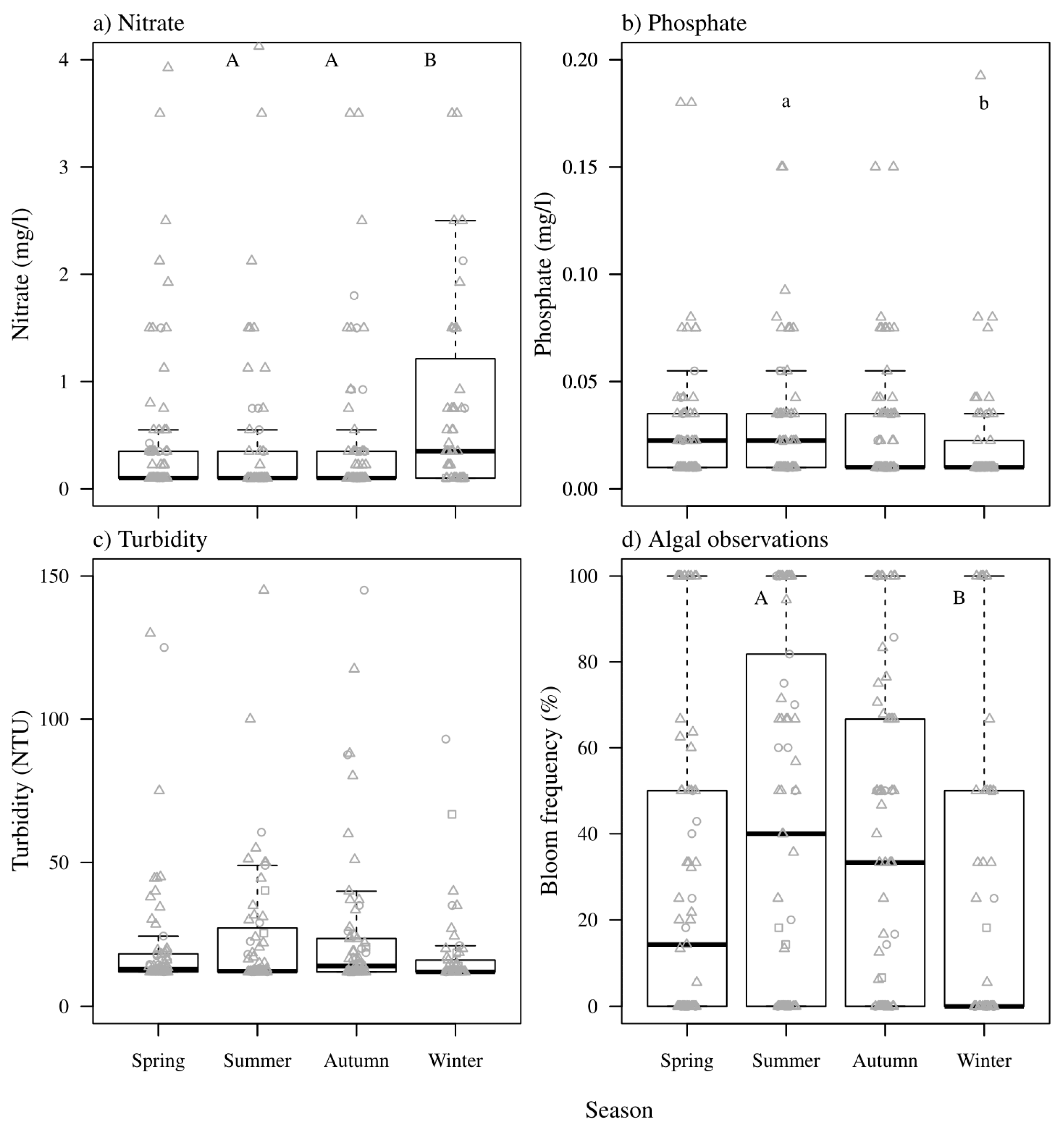
Temporal patterns in water quality were comparable across all study regions (Figure 2) with statistically significant peaks in nitrate concentration during winter with summer and autumn minima (Figure 2a). Phosphate showed less variation across the seasons, although a spring–summer maxima and autumn–winter minima were observed (Figure 2b).
Observations in algal blooms peaked during the summer months where 42.5% of the datasets contained observations of algal blooms, and were significantly less frequently observed in the winter (Figure 2d). North American sites had notably more algal bloom observations during the summer and autumn than European sites where blooms were more frequently observed in the winter (see Supplementary Material Table S2). Turbidity followed a similar trend (Figure 2c). A weak but highly significant correlation was observed at a site level between algal bloom frequency and turbidity (ρ 0.12, P < 0.01).
3.2. Ponds Versus Lakes
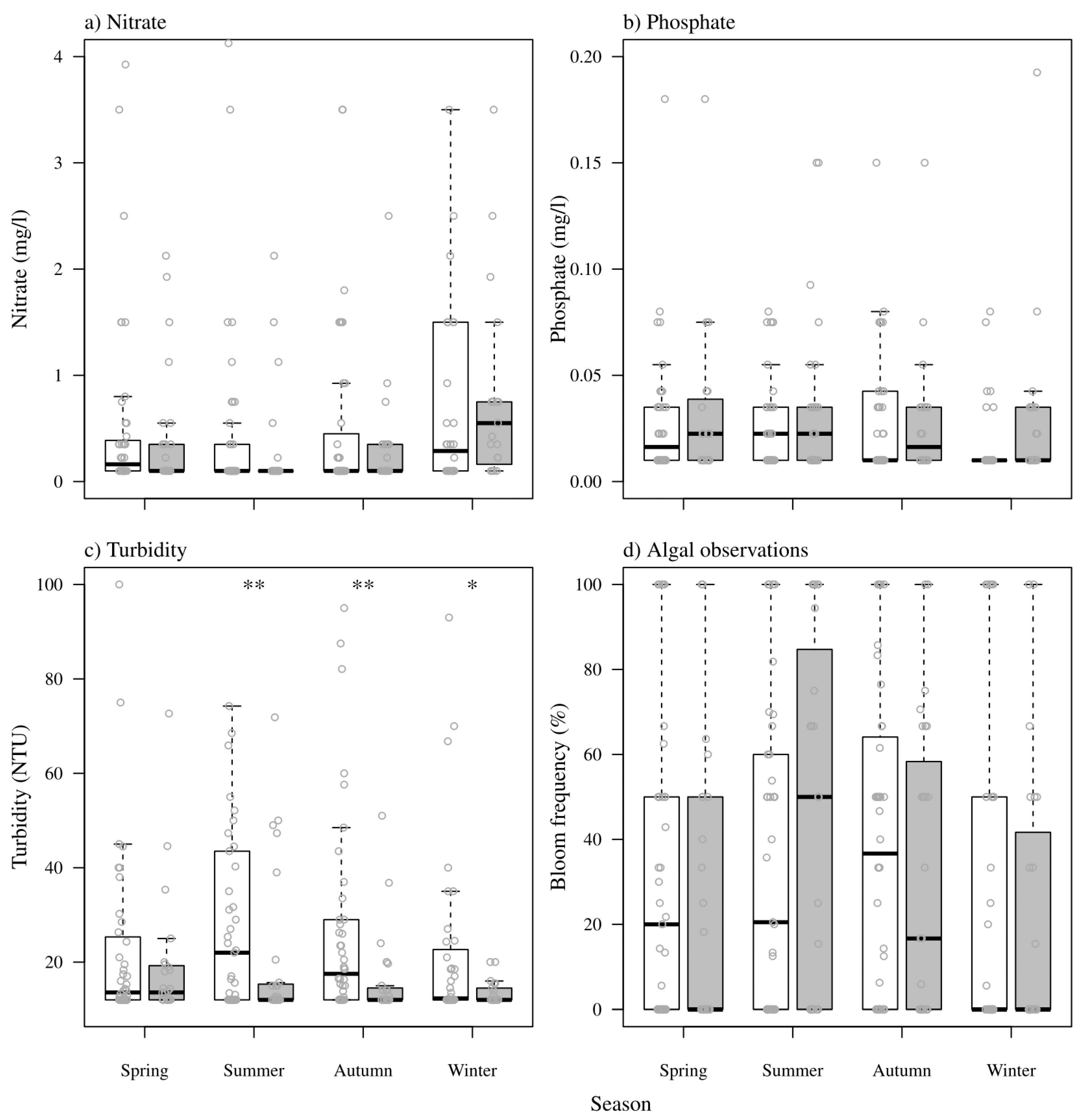
Nutrient concentrations did not show differences between ponds and lakes (Table 3; Figure 3). Turbidity measurements were consistently and significantly (P < 0.05, Mann–Whitney) greater and more wide ranging (P < 0.001, Brown–Forsythe) in ponds (mean 25.3 NTU) than in lakes (mean 17.5 NTU).
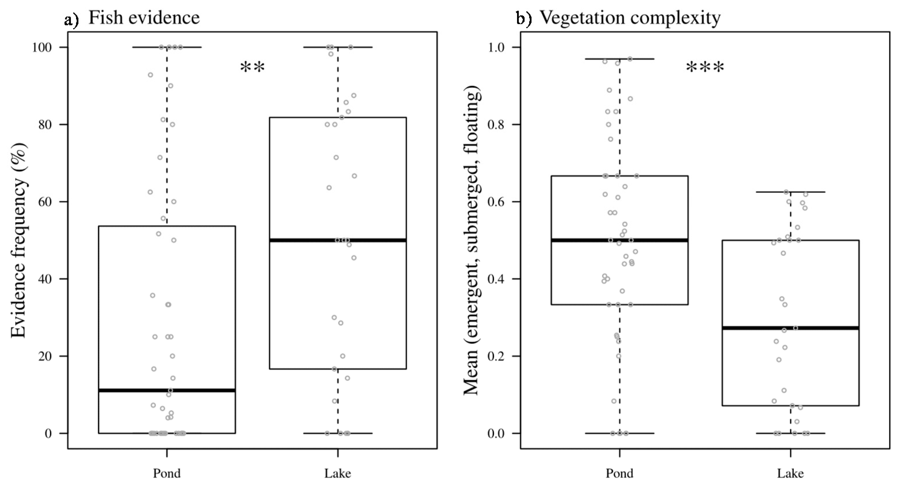
Significant differences were apparent in biological observations, with evidence of fish presence being significantly more likely in larger water bodies. Conversely, complex macrophyte stands were more frequently observed in the smallest water bodies (Figure 4).
3.3. Influence of Urbanisation
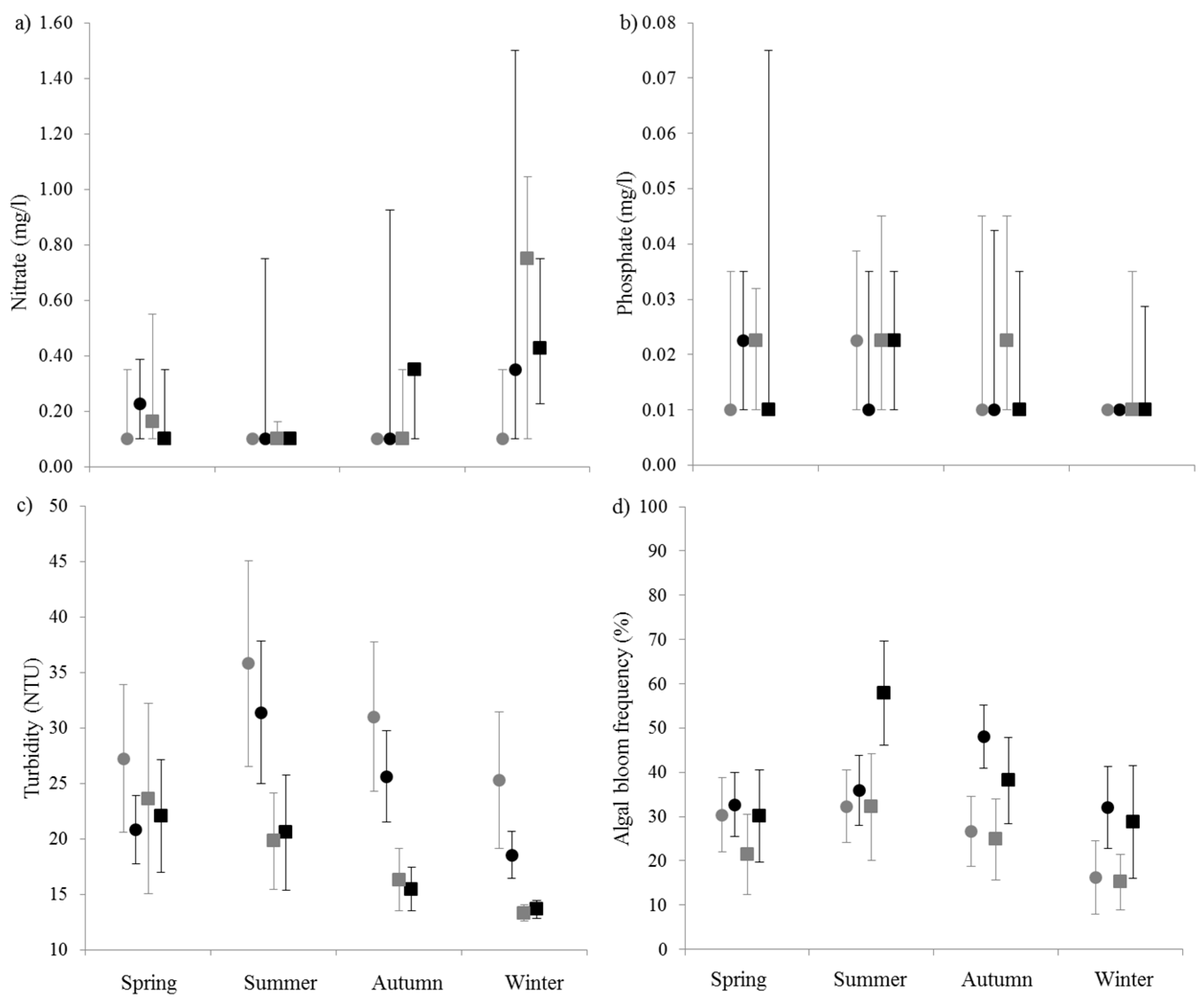
Peri-urban ponds had higher levels of turbidity compared to urban equivalents (Figure 5c); however, this was not found to be significant (Table 4). There were no differences observed between urban and peri-urban lakes. Both ponds and lakes that were located in more urban areas showed a significant increase in algal bloom observations (P < 0.05, Mann–Whitney) (Figure 5d, and Table 5). Other water quality factors did not appear to differ consistently or significantly in response to urbanization.
3.4. Algal Bloom Frequency Across Urban and Peri-Urban Ponds and Lakes
To identify contributing factors to the differences in algal bloom frequency between urban and peri-urban ponds and lakes, multiple linear regression was used, incorporating observational records taken by FWW participants following a multi-model approach. This resulted in 286 model combinations (max. three predictors per model).
Relative variable importance was calculated across all model combinations in relation to algal bloom frequency in urban and peri-urban ponds and lakes (Table 6). The presence of potential point sources of pollution, in particular those identified by citizen scientists as residential or road origin occurred frequently in the top 10 models and were therefore important predictors of algal bloom observations (Table 7). Another reoccurring driver was water level fluctuations. Interestingly, the strength of the association of these drivers with algal blooms was much greater in urban areas (adj. R2 0.24, P < 0.05), than in peri-urban areas, where both variable importance and standardized model coefficient values were low (adj. R2 0.008, P > 0.05). In urban areas, residential discharges showed a positive association with algal bloom frequency while water level fluctuation and road discharges were negative.
4. Discussion
4.1. Physical and Temporal Trends
Data collected by citizen scientists engaged in a global study of freshwater quality identified clear seasonal trends in nutrient status, with peak concentrations of nitrate (N-NO3) during winter periods and phosphate (P-PO4) during spring and summer. Many studies have principally focused on phosphorous owing to its assumed role as a key limiter to algal growth, however, bioavailable nitrogen is also an important driver of aquatic vegetation dynamics [46]. In the present study, winter peaks in nitrate conform to commonly observed patterns (e.g., New York lakes [47]) related to assimilation by algae and other plants throughout the spring and summer growing period and subsequent release into the water column during plant senescence when uptake by phytoplankton and denitrifying bacteria is minimal [48,49].
Summer increases in phosphate accord well with studies of shallow artificial ponds in England [50] and Danish lakes [12] where summer peaks in total phosphorus (TP) were observed. This is frequently suggested to reflect internal loading mechanisms, to which shallow water bodies are more susceptible than deeper water bodies owing to the intense sediment to water column interface [11]. The release of P from the sediment is often in a biologically available form, more readily available for uptake by phytoplankton as indicated by trends in algal bloom frequency [51]. Thus the combination of nutrient sampling kits and observational parameter appeared appropriate for monitoring these trends (accept hypothesis 1). Turbidity (NTU) and algal bloom frequency trends were comparable, likely because of the underlying covariance in the parameters. However, whilst significant, the relationship was not strong.
4.2. Pond vs. Lake
Our study identified consistently higher levels of turbidity within ponds (<2 ha) than lakes. Reasons for this are uncertain, however, could relate to the susceptibility of shallow water bodies to resuspension of sediment following disturbance, e.g., from benthivorous fish [52,53] or wind action [54,55]. Fish presence was typically observed less frequently across repeat visits to smaller water bodies (accept hypothesis 2), in agreement with several other studies of fish abundance [14,15]; however, fish were observed at least once in two-thirds (63%) of ponds. Although species were not identified, the relative density of fish in ponds rather than abundance may be an over-riding influence [56].
Higher macrophyte complexity was also observed within small ponds compared to lakes. A number of studies have highlighted the potential conservation value of ponds [2,3], which is closely linked to macrophyte diversity [19,57]. The present study was limited to the presence of emergent, submerged and floating vegetation based on visual observations, allowing for an underestimation in larger, deeper water bodies, in particular regarding the presence of submerged vegetation.
4.3. Influence of Urbanisation
The influence of urbanization was most pronounced in the frequency of algal bloom observations and there seemed to be a potentially greater influence in ponds (reject hypothesis 3). Eutrophic conditions, a precursor to algal blooms are distinguishing component of the urban stream (urban stream syndrome) [58,59]. This study indicates that it is a characteristic of urban ponds, contributing to the global issue, often associated to lakes [60,61].
The association of algal blooms with a suite of observational parameters indicated that the presence of residential discharges were a driver of algal bloom frequency, with hydrological variability (water level fluctuations) likely to reduce the frequency of algal blooms in the most urban sites. Interestingly, the presence of road discharges were also associated with a reduction. Within our study sites, the presence of residential discharges are more likely to represent phosphate availability as a consequence of domestic waste water and household misconnections [62,63]. Conversely, the negative effect of both water level fluctuation and the presence of road discharge could reflect dilution of nutrients or influence trophic interactions resulting in higher grazing pressure [64,65]. The influence of road discharge is less clear, however the chemical composition of road discharge has been identified to both stimulate (e.g., sodium [66]) or inhibit algal growth (e.g., de-icing salts or herbicide [67]).
Citizen observatories have previously been identified as a potentially powerful tool for the monitoring of algal blooms [35,68] with a suite of applications now having being developed to facilitate their record such as CyanoTRACKER (University of Georgia), Bloomin’ Algae (Centre for Ecology and Hydrology), and bloomWatch (US EPA). The present study suggests that potential local scale drivers may also be monitored by citizen scientists.
5. Conclusions
The incorporation of trained volunteers in the monitoring of inland water bodies presents a potential to broaden our knowledge of their conditions and dynamics [69,70]. This is particularly important for shallow lakes and ponds, which are often overlooked by national and international legislation. In the present study, we demonstrate that observations and measurements of trained citizen scientists can support the identification of temporal and spatial patterns in temperate ponds and lakes.
Most ponds and lakes within urban areas are artificial and often built as part of the supporting infrastructure (e.g., storm water storage, sustainable urban drainage systems). From their local aquatic ecosystems, human populations derive many services which support the economy and wellbeing [71,72]. Direct drivers to the loss of ecosystem integrity will affect their functioning [73,74] and are often difficult to identify. We show that the combination of GIS data with local-scale observational data recorded by the citizen scientists helps to identify local drivers to ecosystem degradation. The results also confirm the role of size in influencing both water quality and ecosystem conditions, again indicating the potential benefits of citizens to cover these often overlooked ecosystems.
Overall, the approach proved promising to both ends, however, citizen science is not without its limitations and its application is not always appropriate. Further, the engagement of citizens can be time-consuming and further research is needed to understand the motivations of local communities with regards to their freshwater resources. We recommend that citizen science provides a useful complementary tool to regulatory and professional monitoring and could act as an early warning system.
Supplementary Materials
The following are available online at https://www.mdpi.com/2073-4441/10/7/839/s1, Table S1: Site summaries for ponds and lakes included within the analysis, Table S2: Average seasonal water quality statistics (±1 SD) for temperate still waters across Oceania (OCN), North America (NAM), and Europe (EUR). Median values displayed for nitrate (N-NO3) and phosphate (P-PO4), mean values for turbidity (NTU) and frequency of algal observations (presence/absence).
Author Contributions
I.T. conceived of the investigation here presented and carried out all statistical analysis and helped train FWW participants. A.C. carried out preliminary investigations of still water FWW data and helped edit and refine the manuscript. S.L. contributed significantly to the FWW citizen science programme and provided advice regarding the aims and objectives of the present study as well as editing capacity.
Funding
This research received no external funding.
Acknowledgments
We sincerely acknowledge the efforts of the Citizen Science Leaders (CSLs) within the HSBC Water Programme and Royal Dutch Shell plc for their dedication and enthusiasm. We also acknowledge the efforts of Jeremy Biggs and Pascale Nicolet (Freshwater Habitats Trust; UK and France), Kim Anema (UNESCO-IHE Institute for Water Education; Netherlands), Eren Turak (Office of Environment and Heritage; Australia), Wade McGillis (Columbia University, USA), and Paul Frost (Canada; Trent University) for their assistance in training and engaging the citizen scientists who participated in the study.
Conflicts of Interest
The authors declare no conflict of interest.
References
- Downing, J.A.; Duarte, C.M. Abundance and size distribution of lakes, ponds and impoundments. In Encyclopedia of Inland Waters; Likens, G.E., Ed.; Elsevier: Oxford, UK, 2009; pp. 469–478. [Google Scholar]
- Williams, P.; Whitfielda, M.; Biggs, J.; Bray, S.; Fox, G.; Nicolet, P.; Sear, D. Comparative biodiversity of rivers, streams, ditches and ponds in an agricultural landscape in Southern England. Biol. Conserv. 2004, 115, 329–341. [Google Scholar] [CrossRef]
- Davies, B.; Biggs, J.; Williams, P.; Whitfield, M.; Nicolet, P.; Sear, D.; Bray, S.; Maund, S. Comparative biodiversity of aquatic habitats in the European agricultural landscape. Agric. Ecosyst. Environ. 2008, 125, 1–8. [Google Scholar] [CrossRef]
- Tranvik, L.J.; Downing, J.A.; Cotner, J.B.; Loiselle, S.A.; Striegl, R.G.; Ballatore, T.J.; Dillon, P.; Finlay, K.; Fortino, K.; Knoll, L.B.; et al. Lakes and reservoirs as regulators of carbon cycling and climate. Limnol. Oceanogr. 2009, 54, 2298–2314. [Google Scholar] [CrossRef] [Green Version]
- Indermuehle, N.; Oertli, B.; Biggs, J.; Céréghino, R.; Grillas, P.; Hull, A.; Nicolet, P.; Scher, O. Pond conservation in Europe: The European Pond Conservation Network ( EPCN ). SIL Proc. 2008, 30, 446–448. [Google Scholar] [CrossRef]
- North American Lake Management Society the Secchi Dip-In. Available online: http://www.secchidipin.org (accessed on 18 November 2017).
- Bonney, R.; Ballard, H.; Jordan, R.; Mccallie, E.; Phillips, T.; Shirk, J.; Wilderman, C. Public Participation in Scientific Research: Defining the Field and Assessing Its Potential for Informal Science Education. In A CAISE Inquiry Group Report; Center for Advancement of Informal Science Education (CAISE): Washington, DC, USA, 2009. [Google Scholar]
- Dickinson, J.L.; Shirk, J.; Bonter, D.; Bonney, R.; Crain, R.L.; Martin, J.; Phillips, T.; Purcell, K. The current state of citizen science as a tool for ecological research and public engagement. Front. Ecol. Environ. 2012, 10, 291–297. [Google Scholar] [CrossRef] [Green Version]
- Gray, S.; Jordan, R.; Crall, A.; Newman, G.; Hmelo-Silver, C.; Huang, J.; Novak, W.; Mellor, D.; Frensley, T.; Prysby, M.; et al. Combining participatory modelling and citizen science to support volunteer conservation action. Biol. Conserv. 2017, 208, 76–86. [Google Scholar] [CrossRef]
- Beklioğlu, M.; Meerhoff, M.; Davidson, T.A.; Ger, K.A.; Havens, K.; Moss, B. Preface: Shallow lakes in a fast changing world. Hydrobiologia 2016, 778, 9–11. [Google Scholar] [CrossRef] [Green Version]
- Scheffer, M. Ecology of Shallow Lakes, 1st ed.; Chapman and Hall: London, UK, 1998. [Google Scholar]
- Jeppesen, E.; Jensen, J.P.; Søndergaard, M.; Lauridsen, T.; Pedersen, L.J.; Jensen, L. Top-down control in freshwater lakes: The role of nutrient state, submerged macrophytes and water depth. Hydrobiologia 1997, 342, 151–164. [Google Scholar] [CrossRef]
- Pettersson, K. Mechanisms for internal loading of phosphorus in lakes. Hydrobiologia 1998, 373, 21–25. [Google Scholar] [CrossRef]
- Søndergaard, M.; Jeppesen, E.; Jensen, J.P.; Sondergaard, M. Pond or lake: Does it make any difference? Arch. Hydrobiol. 2005, 162, 143–165. [Google Scholar] [CrossRef]
- Scheffer, M.; Van Geest, G.J.; Zimmer, K.; Jeppesen, E.; Sondergaard, M.; Butler, M.G.; Hanson, M.A.; Declerck, S.; De Meester, L. Small habitat size and isolation can promote species richness: Second-order effects on biodiversity in shallow lakes and ponds. Oikos 2006, 112, 227–231. [Google Scholar] [CrossRef]
- Hassall, C. The ecology and biodiversity of urban ponds. Wiley Interdiscip. Rev. Water 2014, 1, 187–206. [Google Scholar] [CrossRef] [Green Version]
- Walsh, C.J.; Roy, A.H.; Feminella, J.W.; Cottingham, P.D.; Groffman, P.M.; Morgan, R.P. The urban stream syndrome: Current knowledge and the search for a cure. J. N. Am. Benthol. Soc. 2005, 24, 706–723. [Google Scholar] [CrossRef]
- Hill, M.J.; Biggs, J.; Thornhill, I.; Briers, R.A.; Gledhill, D.G.; White, J.C.; Wood, P.J.; Hassall, C. Urban ponds as an aquatic biodiversity resource in modified landscapes. Glob. Chang. Biol. 2016, 23, 986–999. [Google Scholar] [CrossRef] [PubMed] [Green Version]
- Thornhill, I.; Batty, L.; Death, R.G.; Friberg, N.R.; Ledger, M.E. Local and landscape scale determinants of macroinvertebrate assemblages and their conservation value in ponds across an urban land-use gradient. Biodivers. Conserv. 2017, 26, 1065–1086. [Google Scholar] [CrossRef] [Green Version]
- Wood, P.J.; Barker, S. Old industrial mill ponds: A neglected ecological resource. Appl. Geogr. 2000, 20, 65–81. [Google Scholar] [CrossRef]
- Peretyatko, A.; Teissier, S.; Backer, S.; Triest, L. Restoration potential of biomanipulation for eutrophic peri-urban ponds: The role of zooplankton size and submerged macrophyte cover. Hydrobiologia 2009, 634, 125–135. [Google Scholar] [CrossRef]
- Biggs, J.; Fox, G.; Nicolet, P.; Walker, D.; Whitfield, M.; Williams, P. A Guide to the Methods of the National Pond Survey; Pond Action: Oxford, UK, 1998. [Google Scholar]
- Conrad, C.C.; Hilchey, K.G. A review of citizen science and community-based environmental monitoring: Issues and opportunities. Environ. Monit. Assess. 2011, 176, 273–291. [Google Scholar] [CrossRef] [PubMed]
- Thornhill, I.; Loiselle, S.; Lind, K.; Ophof, D. The citizen science opportunity for researchers and agencies. Bioscience 2016, 66, 720–721. [Google Scholar] [CrossRef]
- Whitelaw, G.; Vaughan, H.; Craig, B.; Atkinson, D. Establishing the Canadian Community Monitoring Network. Environ. Monit. Assess. 2003, 88, 409–418. [Google Scholar] [CrossRef] [PubMed]
- Olson, D.M.; Dinerstein, E.; Wikramanayake, E.D.; Burgess, N.D.; Powell, G.V.N.; Underwood, E.C.; D’Amico, J.A.; Itoua, I.; Strand, H.E.; Morrison, J.C.; et al. Terrestrial ecoregions of the world: A new map of life on Earth. Bioscience 2001, 51, 933–938. [Google Scholar] [CrossRef]
- Thornhill, I.; Ho, J.G.; Zhang, Y.; Li, H.; Ho, K.C.; Miguel-Chinchilla, L.; Loiselle, S.A. Prioritising local action for water quality improvement using citizen science; a study across three major metropolitan areas of China. Sci. Total Environ. 2017, 584–585, 1268–1281. [Google Scholar] [CrossRef] [PubMed]
- Rice, E.W.; Baird, R.B.; Eaton, A.D.; Clesceri, L.S. Standard Methods for the Examination of Water and Wastewater, 22nd ed.; American Public Health Association: Washington, DC, USA, 2012. [Google Scholar]
- World Weather Online World Weather Online (Monthly Climate Averages). Available online: http://www.worldweatheronline.com/ (accessed on 7 April 2018).
- Ellis, P.S.; Shabani, A.M.H.; Gentle, B.S.; McKelvie, I.D. Field measurement of nitrate in marine and estuarine waters with a flow analysis system utilizing on-line zinc reduction. Talanta 2011, 84, 98–103. [Google Scholar] [CrossRef] [PubMed]
- Strickland, J.D.H.; Parsons, T. A Practical Handbook of Seawater Analysis; Fisheries Research Board of Canada: Ottawa, ON, Canada, 1972. [Google Scholar]
- Berti, G.; Fossati, P.; Tarenghi, G.; Musitelli, C.; Melzi d’Eril, G.V. Enzymatic colorimetric method for the determination of inorganic phosphorus in serum and urine. J. Clin. Chem. Clin. Biochem. 1988, 26, 399–404. [Google Scholar] [CrossRef] [PubMed]
- Dahlgren, R.; Nieuwenhuyse, E.; Van Litton, G. Transparency tube provides reliable water-quality measurements. Calif. Agric. 2008, 58, 149–153. [Google Scholar] [CrossRef]
- Tyler, J.E. The Secchi disk. Limnol. Oceanogr. 1968, 13. [Google Scholar] [CrossRef]
- Castilla, E.P.; Cunha, D.G.F.; Lee, F.W.F.; Loiselle, S.; Ho, K.C.; Hall, C. Quantification of phytoplankton bloom dynamics by citizen scientists in urban and peri-urban environments. Environ. Monit. Assess. 2015, 187. [Google Scholar] [CrossRef] [PubMed]
- Biggs, J.; McGoff, E.; Ewald, N.; Dunn, F.; Nicolet, P.; Williams, P. Clean Water for Wildlife. In Using PackTest Nitrate and Phosphate Test Kits to Find Clean Water and Assess the Extent of Pollution; Freshwater Habitats Trust: Oxford, UK, 2016. [Google Scholar]
- Miguel-Chinchilla, L.; Thornhill, I.; Baruch, A.; Loiselle, S.A. FreshWater Watch Methods (draft); Freshwater Habitats Trust: Oxford, UK, 2017. [Google Scholar]
- Muneoka, T. Evaluation of Nitrate Pollution in River Water at Agricultural Watershed; Freshwater Habitats Trust: Oxford, UK, 2014; pp. 51–56. [Google Scholar]
- Biggs, J.; Williams, P.; Whitfield, M.; Nicolet, P.; Weatherby, A. 15 years of pond assessment in Britain: Results and lessons learned from the work of Pond Conservation. Aquat. Conserv. Mar. Freshw. Ecosyst. 2005, 15, 693–714. [Google Scholar] [CrossRef]
- Latham, J.; Cumani, R.; Rosati, I.; Bloise, M. FAO Global Land Cover (GLC-SHARE) Beta-Release 1.0 Database; Land and Water Division: Rome, Italy, 2014. [Google Scholar]
- CIESIN. Gridded Population of the World, Version 4 (GPWv4). Preliminary Release 2 (2010) 2014.. Available online: http://sedac.ciesin.columbia.edu/data/collection/gpw-v4 (accessed on 14 June 2018).
- R Core Team R: A Language and Environment for Statistical Computing; The R Foundation for Statistical Computing: Vienna, Austria, 2017; ISBN 3-900051-07-0.
- Burnham, K.P.; Anderson, D.R. Model Selection and Multimodel Inference: A Practical Information-Theoretic Approach, 2nd ed.; Springer: New York, NY, USA, 2002; ISBN 0387953647. [Google Scholar]
- Whittingham, M.J.; Stephens, P.A.; Bradbury, R.B.; Freckleton, R.P. Why do we still use stepwise modelling in ecology and behaviour? J. Anim. Ecol. 2006, 75, 1182–1189. [Google Scholar] [CrossRef] [PubMed] [Green Version]
- Grueber, C.E.; Nakagawa, S.; Laws, R.J.; Jamieson, I.G. Multimodel inference in ecology and evolution: Challenges and solutions. J. Evol. Biol. 2011, 24, 699–711. [Google Scholar] [CrossRef] [PubMed]
- Brönmark, C.; Hansson, L.-A. The Biology of Lakes and Ponds; Oxford University Press: Oxford, UK, 2008. [Google Scholar]
- Stewart, K.M.; Markello, S.J. Seasonal variations in concentrations of nitrate and total phosphorus, and calculated nutrient loading for six lakes in western New York. Hydrobiologia 1974, 44, 61–89. [Google Scholar] [CrossRef]
- Wetzel, R.G. Limnology: Lake and River Ecosystems; Academic Press: Cambridge, MA, USA, 2001; ISBN 9780127447605. [Google Scholar]
- Ansari, A.A.; Singh Gill, S.; Lanza, G.R.; Rast, W. Eutrophication: Causes; Springer: New York, NY, USA, 2011; ISBN 9789048196241. [Google Scholar]
- Bennion, H.; Smith, M.A. Variability in the water chemistry of shallow ponds in southeast England, with special reference to the seasonality of nutrients and implications for modelling trophic status. Hydrobiologia 2000, 436, 145–158. [Google Scholar] [CrossRef]
- Nürnberg, G.K. Assessing internal phosphorus load—Problems to be solved. Lake Reserv. Manag. 2009, 25, 419–432. [Google Scholar] [CrossRef]
- Breukelaar, A.W.; Lammens, E.H.R.R.; Breteler, J.G.P.K.; Tatrai, I. Effects of benthivorous bream (Abramis brama) and carp (Cyprinus carpio) on sediment resuspension and concentrations of nutrients and chlorophyll a. Freshw. Biol. 1994, 32, 113–121. [Google Scholar] [CrossRef]
- Cline, J.M.; East, T.L.; Threlkeld, S.T. Fish interactions with the sediment-water interface. Hydrobiologia 1994, 275–276, 301–311. [Google Scholar] [CrossRef]
- Globevnik, L.; Kirn, T. Small Water Bodies—Assessment of Status and Threats of Standing Small Water Bodies. IERS, 2009. Available online: http://icm.eionet.europa.eu/ETC_Reports/Assessment%20of%20status%20and%20threats%20of%20standing%20small%20water%20bodies.pdf (accessed on 14 June 2018).
- De Meester, L.; Declerck, S.; Stoks, R.; Louette, G.; Van de Meutter, F.; De Bie, T.; Michels, E.; Brendonck, L. Ponds and pools as model systems in conservation biology, ecology and evolutionary biology. Aquat. Conserv. Mar. Freshw. Ecosyst. 2005, 725, 715–725. [Google Scholar] [CrossRef]
- Olin, M.; Rask, M.; Ruuhljärvi, J.; Kurkilahti, M.; Ala-Opas, P.; Ylönen, O. Fish community structure in mesotrophic and eutrophic lakes of southern Finland: The relative abundances of percids and cyprinids along a trophic gradient. J. Fish Biol. 2002, 60, 593–612. [Google Scholar] [CrossRef]
- Gledhill, D.G.; James, P.; Davies, D.H. Pond density as a determinant of aquatic species richness in an urban landscape. Landsc. Ecol. 2008, 23, 1219–1230. [Google Scholar] [CrossRef]
- Wenger, S.J.; Roy, A.H.; Jackson, C.R.; Bernhardt, E.S.; Carter, T.L.; Filoso, S.; Gibson, C.A.; Hession, W.C.; Kaushal, S.S.; Martí, E.; et al. Twenty-six key research questions in urban stream ecology: An assessment of the state of the science. J. N. Am. Benthol. Soc. 2009, 28, 1080–1098. [Google Scholar] [CrossRef]
- Walsh, C.J. Urban impacts on the ecology of receiving waters: A framework for assessment, conservation and restoration. USGS 2000, 431, 107–114. [Google Scholar]
- Golterman, H.L.; Oude, N.T. Eutrophication of Lakes, Rivers and Coastal Seas. In Water Pollution; Springer: Berlin/Heidelberg, Germany, 1991; pp. 79–124. [Google Scholar]
- Brooks, B.W.; Lazorchak, J.M.; Howard, M.D.A.; Johnson, M.-V.V.; Morton, S.L.; Perkins, D.A.K.; Reavie, E.D.; Scott, G.I.; Smith, S.A.; Steevens, J.A. Are harmful algal blooms becoming the greatest inland water quality threat to public health and aquatic ecosystems? Environ. Toxicol. Chem. 2016, 35, 6–13. [Google Scholar] [CrossRef] [PubMed]
- Ellis, J.B.B.; Butler, D. Surface water sewer misconnections in England and Wales: Pollution sources and impacts. Sci. Total Environ. 2015, 526, 98–109. [Google Scholar] [CrossRef] [PubMed]
- Revitt, D.M.; Ellis, J.B. Urban surface water pollution problems arising from misconnections. Sci. Total Environ. 2016, 551–552, 163–174. [Google Scholar] [CrossRef] [PubMed]
- Naselli-Flores, L.; Barone, R. Importance of water-level fluctuation on population dynamics of cladocerans in a hypertrophic reservoir (Lake Arancio, south-west Sicily, Italy). Hydrobiologia 1997, 223–232. [Google Scholar] [CrossRef]
- Scheffer, M.; Hosper, S.H.; Meijer, M.L.; Moss, B.; Jeppesen, E. Alternative equilibria in shallow lakes. Trends Ecol. Evol. 1993, 8, 275–279. [Google Scholar] [CrossRef]
- Ramakrishna, D.M.; Viraraghavan, T. Environmental impact of chemical deicers—A review. Water Air Soil Pollut. 2005, 166, 49–63. [Google Scholar] [CrossRef]
- Huang, X.; Pedersen, T.; Fischer, M.; White, R.; Young, T.M. Herbicide Runoff along Highways. 1. Field Observations. Environ. Sci. Technol. 2004, 38, 3263–3271. [Google Scholar] [CrossRef] [PubMed]
- Cunha, D.G.F.; Casali, S.P.; de Falco, P.B.; Thornhill, I.; Loiselle, S.A. The contribution of volunteer-based monitoring data to the assessment of harmful phytoplankton blooms in Brazilian urban streams. Sci. Total Environ. 2017, 584–585, 586–594. [Google Scholar] [CrossRef] [PubMed]
- Bonney, R.; Cooper, C.B.; Dickinson, J.; Kelling, S.; Phillips, T.; Rosenberg, K.V.; Shirk, J. Citizen Science: A Developing Tool for Expanding Science Knowledge and Scientific Literacy. Bioscience 2009, 59, 977–984. [Google Scholar] [CrossRef] [Green Version]
- Buytaert, W.; Zulkafli, Z.; Grainger, S.; Acosta, L.; Alemie, T.C.; Bastiaensen, J.; De Bièvre, B.; Bhusal, J.; Clark, J.; Dewulf, A.; et al. Citizen science in hydrology and water resources: Opportunities for knowledge generation, ecosystem service management, and sustainable development. Front. Earth Sci. 2014, 2, 1–21. [Google Scholar] [CrossRef]
- Erwin, K.L. Wetlands and global climate change: The role of wetland restoration in a changing world. Wetl. Ecol. Manag. 2009, 17, 71–84. [Google Scholar] [CrossRef]
- De Bello, F.; Lavorel, S.; Díaz, S.; Harrington, R.; Cornelissen, J.H.C.; Bardgett, R.D.; Berg, M.P.; Cipriotti, P.; Feld, C.K.; Hering, D.; et al. Towards an assessment of multiple ecosystem processes and services via functional traits. Biodivers. Conserv. 2010, 19, 2873–2893. [Google Scholar] [CrossRef]
- Diaz, S.; Cabido, M. Vive la difference: Plant functional diversity matters to ecosystem processes. Trends Ecol. Evol. 2001, 16, 646–655. [Google Scholar] [CrossRef]
- Gessner, M.O.; Inchausti, P.; Persson, L.; Raffaelli, D.G.; Giller, P.S. Biodiversity effects on ecosystem functioning: Insights from aquatic systems. Oikos 2004, 3, 419–422. [Google Scholar] [CrossRef]
Figure 1.
Distribution of 75 ponds and lakes used in the present study located in temperate biomes across three continents (six countries).
Figure 1.
Distribution of 75 ponds and lakes used in the present study located in temperate biomes across three continents (six countries).

Figure 2.
Comparison of nutrient concentrations (a,b), turbidity (c) and algal bloom observations (d) across seasons and continents within still waters (ponds and lakes). Lettering (e.g., A, B) denotes significant differences between seasons (Kruskal–Wallis post hoc Dunn test, where upper case = P < 0.05, lower case = P < 0.1). Symbols are median seasonal values from individual sites: □ = Oceania, ○ = North America, ∆ = Europe.

Figure 3.
Comparison of nutrient concentrations, turbidity, and algal bloom observations across seasons within ponds (hollow boxes) or lakes (grey boxes). Asterisks denote significant differences between ponds and lakes (Kruskal–Wallis post hoc Dunn test, ** = P < 0.01, * = P < 0.05).
Figure 3.
Comparison of nutrient concentrations, turbidity, and algal bloom observations across seasons within ponds (hollow boxes) or lakes (grey boxes). Asterisks denote significant differences between ponds and lakes (Kruskal–Wallis post hoc Dunn test, ** = P < 0.01, * = P < 0.05).

Figure 4.
Comparison of physical characteristics between ponds (<2 ha) and lakes (>2 ha). Asterisks indicate significant differences (Mann–Whitney test, ** P < 0.05, *** P < 0.01).
Figure 4.
Comparison of physical characteristics between ponds (<2 ha) and lakes (>2 ha). Asterisks indicate significant differences (Mann–Whitney test, ** P < 0.05, *** P < 0.01).

Figure 5.
Comparison of trends in (a) nitrate, (b) phosphate, (c) turbidity, (d) algal bloom frequency, across seasons between peri-urban (grey) and urban (black), ponds (circles), and lakes (squares). Median values (and inter-quartile range) for nutrients, mean (and standard error) for turbidity and algal bloom frequency.


Table 1.
Data summary for FreshWater Watch temperate still water sites and samples (in parentheses) between 1 June 2014 and 31 May 2016.
Table 1.
Data summary for FreshWater Watch temperate still water sites and samples (in parentheses) between 1 June 2014 and 31 May 2016.
| North America | Europe | Oceania | Totals | |
|---|---|---|---|---|
| <0.2 ha | 0 (0) | 15 (135) | 0 (0) | 15 (135) |
| >0.2 ha <2 ha | 7 (113) | 22 (543) | 2 (29) | 31 (685) |
| >2 ha <20 ha | 2 (33) | 20 (215) | 1 (43) | 23 (291) |
| >20 ha | 1 (10) | 5 (71) | 0 (0) | 6 (81) |
| Totals | 10 (156) | 63 (964) | 3 (72) | 75 (1192) |
Table 2.
Quality assurance and control framework within the FreshWater Watch programme.
| Prevention | Detection |
|---|---|
| Training | Feedback |
| Train-the-trainer events | Automatic (qualitative and quantitative) |
| One-day experiential learning event | Principal Investigator (local partner) |
| Mandatory research quiz | Global research team (Earthwatch) |
| Recording form instruction | Quality control |
| Voluntary online modular learning | 10% validity check by PI [28] |
| Method testing Accredited laboratory [36,37] Independent testing [33,38] | Manual database checking protocol [37] Photographs |
Table 3.
Comparison of average of and variance in nutrient concentrations, turbidity, and algal bloom occurrence between ponds (<2 ha) vs. lakes (>2 ha). Numbers in parentheses are ±1 SD.
Table 3.
Comparison of average of and variance in nutrient concentrations, turbidity, and algal bloom occurrence between ponds (<2 ha) vs. lakes (>2 ha). Numbers in parentheses are ±1 SD.
| Ponds | Lakes | Mann–Whitney p | Brown–Forsyth p | |
|---|---|---|---|---|
| Nitrate (mg/L) | 0.1 (0.75) | 0.1 (0.44) | 0.55 | 0.54 |
| Phosphate (mg/L) | 0.01 (0.02) | 0.01 (0.03) | 0.86 | 0.85 |
| Turbidity (NTU) | 17.0 (22.9) | 13.4 (9.9) | 0.01 ** | <0.001 ** |
| Bloom frequency (%) | 32.0 (27.6) | 30.5 (26.9) | 0.80 | 0.56 |
Note: Asterisks indicate significant difference where ** = P < 0.01.
Table 4.
Comparison of nutrient concentrations, turbidity, and algal bloom occurrence between urban vs. peri-urban ponds. Numbers in parentheses are ±1 SD.
Table 4.
Comparison of nutrient concentrations, turbidity, and algal bloom occurrence between urban vs. peri-urban ponds. Numbers in parentheses are ±1 SD.
| Peri-Urban | Urban | Mann-Whitney p | Brown–Forsyth p | |
|---|---|---|---|---|
| Nitrate (mg/L) | 0.1 (0.74) | 0.1 (0.77) | 0.19 | 0.59 |
| Phosphate (mg/L) | 0.01 (0.03) | 0.01 (0.04) | 0.07 * | 0.11 |
| Turbidity (NTU) | 30.0 (27.1) | 24.7 (19.0) | 0.91 | 0.18 |
| Bloom frequency (%) | 25.1 (26.2) | 38.6 (27.8) | 0.09 * | 0.54 |
Note: Asterisks indicate significant difference where * = P < 0.5.
Table 5.
Comparison of average of and variance in nutrient concentrations, turbidity and algal bloom occurrence between urban vs. peri-urban lakes and ponds. Numbers in parentheses are ±1 SD.
Table 5.
Comparison of average of and variance in nutrient concentrations, turbidity and algal bloom occurrence between urban vs. peri-urban lakes and ponds. Numbers in parentheses are ±1 SD.
| Peri-Urban | Urban | Mann–Whitney p | Brown–Forsyth p | |
|---|---|---|---|---|
| Nitrate (mg/L) | 0.1 (0.63) | 0.1 (0.66) | 0.44 | 0.71 |
| Phosphate (mg/L) | 0.01 (0.03) | 0.01 (0.02) | 0.38 | 0.15 |
| Turbidity (NTU) | 25.4 (22.6) | 22.8 (16.8) | 0.74 | 0.25 |
| Bloom frequency (%) | 24.7 (24.5) | 38.6 (28.3) | 0.03 ** | 0.22 |
Note: Asterisks indicate significant difference where ** = P < 0.01.
Table 6.
Comparison of nutrient concentrations, turbidity and algal bloom occurrence between urban vs. peri-urban lakes. Numbers in parentheses are ±1 SD.
Table 6.
Comparison of nutrient concentrations, turbidity and algal bloom occurrence between urban vs. peri-urban lakes. Numbers in parentheses are ±1 SD.
| Peri-Urban | Urban | Mann–Whitney p | Brown–Forsyth p | |
|---|---|---|---|---|
| Nitrate (mg/L) | 0.1 (0.47) | 0.1 (0.41) | 0.73 | 0.70 |
| Phosphate (mg/L) | 0.01 (0.04) | 0.01 (0.2) | 0.47 | 0.86 |
| Turbidity (NTU) | 18.7 (11.7) | 19.2 (11.4) | 0.72 | 0.85 |
| Bloom frequency (%) | 24.1 (22.6) | 38.5 (30.4) | 0.19 | 0.20 |
Table 7.
Multi-model inference results using an Akaike information criterion (AICc)—information theoretic (AIC–IT) approach for algal observations in urban and peri-urban ponds and lakes. Table limited to the predictors occurring in the top 10 models. Asterix indicates significance level within the AIC-best model where P < 0.05.
| Peri-Urban Ponds and Lakes | Urban Ponds and Lakes | ||||||
|---|---|---|---|---|---|---|---|
| Predictor | βj | w + (j) | # | Predictor | βj | w + (j) | # |
| Dis_Road | 0.078 | 0.33 | 8 | Dis_Res * | 0.300 | 0.67 | 9 |
| Lev_Flu | 0.054 | 0.28 | 3 | Lev_Flu * | −0.138 | 0.44 | 3 |
| Dis_Tot | 0.063 | 0.28 | 2 | Dis_Road * | −0.185 | 0.43 | 5 |
| Veg_Flt | −0.050 | 0.27 | 8 | Dist_Tot | −0.021 | 0.34 | 5 |
| Veg_Emer | −0.046 | 0.26 | 2 | Bnk_Bar | −0.070 | 0.25 | 3 |
| LU_For | −0.031 | 0.21 | 1 | Veg_Flt | 0.029 | 0.15 | 2 |
| Fish | 0.028 | 0.21 | 1 | Bnk_Tree | −0.031 | 0.14 | 1 |
| LU_UrbRes | −0.026 | 0.21 | 3 | LU_UrbRes | 0.028 | 0.14 | 2 |
| Bnk_Grass | −0.025 | 0.20 | - | LU_UP | −0.006 | 0.10 | - |
| Dis_Res | 0.020 | 0.19 | - | Veg_Sub | 0.001 | 0.09 | - |
Dis_Road = road discharge, Dis_Res = residential discharge, Lev_Flu = water level fluctuation, Dis_Tot = total number of discharges, Veg_Flt = floating vegetation Veg_Emer = emergent vegetation, Bnk_Bar = bare bank, LU_For = forested land-use, Bnk_Tree = bankside trees, LU_UrbRes = urban/residential land-use, Bnk_Grass = bank side grass, LU_UP = urban park land-use, Veg_Sub = submerged vegetation. Asterisks indicate statistically significant predictors where * = P < 0.5.
© 2018 by the authors. Licensee MDPI, Basel, Switzerland. This article is an open access article distributed under the terms and conditions of the Creative Commons Attribution (CC BY) license (http://creativecommons.org/licenses/by/4.0/).
Share and Cite
MDPI and ACS Style
Thornhill, I.; Chautard, A.; Loiselle, S. Monitoring Biological and Chemical Trends in Temperate Still Waters Using Citizen Science. Water 2018, 10, 839. https://doi.org/10.3390/w10070839
AMA Style
Thornhill I, Chautard A, Loiselle S. Monitoring Biological and Chemical Trends in Temperate Still Waters Using Citizen Science. Water. 2018; 10(7):839. https://doi.org/10.3390/w10070839
Chicago/Turabian StyleThornhill, Ian, Alice Chautard, and Steven Loiselle. 2018. "Monitoring Biological and Chemical Trends in Temperate Still Waters Using Citizen Science" Water 10, no. 7: 839. https://doi.org/10.3390/w10070839
Note that from the first issue of 2016, this journal uses article numbers instead of page numbers. See further details here.