Circulation Characteristic Analysis of Implied Water Flow Based on a Complex Network: A Case Study for Beijing, China

Abstract

Water and energy are two indispensable resources in national economic production. Water is circulated among economic sectors through products or services; however, indirect water consumption calculated by the input–output method fails to reflect the implied water utilised during energy consumption. This study combined the ecological input–output method with a complex network model to analyse the embodied energy intensity (EEI) and the implied water intensity of embodied energy (IWIEE), and then constructed and analysed the implied water circulation network (IWCN) of 40 sectors in 2007, 2010, and 2012 in Beijing. The results indicate that the energy consumption of all of the sectors is mainly embodied in the transfer of the external provinces of China, and the variation trend of the implied water intensity of the embodied energy is consistent with the embodied energy intensity. The implied water circulation networks had small-world characteristics, indicating that water-saving effects in key sectors can quickly spread to other sectors. However, this may also result in a corresponding negative impact if water shortages occur in these sectors, due to the same spreading effect. The node strength, eigenvector centrality, key edge, and key indirect water flow path were selected as indicators to measure key sectors. Finally, water-saving measures and suggestions were proposed according to the complex network characteristics.

1. Introduction

Water is an indispensable natural resource for the development of the national economy. Recently, various industries in many countries and regions around the world have suffered from water shortages [1,2]. In China, especially in the eastern and northern provinces, moderate to severe water shortages have occurred successively and affected regional municipal, industrial, and agricultural developments [3]. Furthermore, the development of the national economy requires energy. Rapid economic growth and urbanisation has led to a rapid increase in energy consumption in China [4]; the total consumption increased from 987 million tons of coal equivalent (Mtce) in 1990 to 4360 Mtce in 2016, with an average annual growth rate of 9.7% [5], making China the most energy-consuming country in the world [6]. Both water and energy are important aspects of industrial production. However, in water shortage areas, water consumption during energy production undoubtedly aggravates the already severe water shortage. Therefore, as well as direct water consumption, further consideration of water consumption during energy production has important and practical significance when comprehensively analysing the relationship between water and energy.

Previous studies on resource consumption in industrial sectors have mainly focussed on the input–output method [7,8,9,10], which analyses the indirect consumption that is circulated within products or services among different regions and sectors. However, there is typically a deficiency in this type of research, because the simulation results can only be applied to the final consumption product; they cannot be applied to the analysis of the intermediate input and output. Based on this idea, Chen et al. proposed an ecological input–output method that is fundamentally different from the traditional environmental input–output method [11]. This method accounts for the resource intensity of sectors based on the balance and flow of resources in the system, and it effectively overcomes the drawbacks of the traditional environmental input–output method. The results obtained can not only be used to calculate the resources embodied in the final consumption, they can also can be used to calculate the resources embodied in the intermediate input. This greatly expands the scope of application of the input–output simulation, and provides a more complete and reliable theoretical method for resource accounting at various scales [12]. This method was originally used to calculate the carbon emissions of buildings [13], and then was widely used in calculations of various ecological embodied resources such as greenhouse gas emissions [11,14], water resources [15,16], energy consumption [17,18] and emergy [19,20]. The research scale involves macroeconomies at different levels, such as at the world scale [21,22], national scale [23,24,25], provincial scale [16], and city scale [15,26].

Resources circulate among various sectors and regions through products or services, and evolve into networks with complicated circulation relationships. The results of the ecological input–output method cannot reflect the structural characteristics of the circulation network; however, system structural analysis can effectively identify key sectors and interdependence among the sectors during resource consumption, which is a prerequisite for solving resource-related problems [27]. The complex network model is a powerful tool in system structure analyses that regards industrial sectors as nodes, and flows between the sectors as edges. To gain a better understanding of the nature of the network [28,29,30], it can find collectors and distributors that play a major role in the network, and explore potential dependencies among sectors to better manage and control the allocation of limited resources. This model has reached maturity in its application in the field of resource trade, such as in the world-scale virtual water trade [31], international oil trade [32,33,34], international natural gas trade [35,36], fossil energy trade [37,38], comprehensive energy trade [39], national scale embodied exergy trade [40], and embodied rare earths trade [41].

The input–output method and the complex network model provide appropriate solutions for the quantitative and structural analysis of energy and water consumption. However, most studies have focussed on a single aspect of water or energy; none of these studies have considered the indirect water consumption or explored the inherent impacts of regional energy consumption on water.

Beijing is the capital of China, and the country’s political, economic, and cultural centre. It is located in the Haihe River basin, which has experienced the most serious water resource shortage of the seven river basins, because water resource shortages and water quality shortages coexist in this basin. The total amount of water resource is unstable due to factors such as human activities and the fluctuation of climatic conditions. The amount of groundwater resource in 2016 was 2.1 billion m³ [42], which was a notable reduction from the 1980 amount of 9.1 billion m³. The per capita water resource was 161 m³, which was far below the global water shortage warning line of 1000 m³. As a severe water shortage area, Beijing’s economic and social development is severely restricted by a lack of water resources.

In terms of energy consumption, the total energy consumption increased from 27.1 Mtce in 1990 to 69.6 Mtce in 2016 [5], with an average annual growth rate of 6.1%. Energy consumption in the tertiary industry and the public sector has increased year to year. Both primary energy and fossil energy consumption make up large proportions of the total energy consumption. Energy efficiency has improved in recent years, but there is still a gap between China and other developed countries. Recently, the increase in widespread haze and energy consumption have been inextricably linked. Therefore, this study selected Beijing as the study area, and combines the ecological input–output method with a complex network model for the analysis. The ecological input–output method is used to calculate the embodied energy intensity (EEI) in each industrial sector (EEI is defined as the total amount of energy consumed directly and indirectly by the unit product or service throughout the life cycle) [18,43]. On this basis, the implied water of embodied energy (IWEE) is also calculated, whereby IWEE is defined as the amount of water consumed per unit of embodied energy during the production process. Then, implied water circulation networks (IWCNs) in Beijing are constructed using a complex network model. Finally, countermeasures for sustainable water utilisation are proposed through the exploration of key nodes and edges in the network. The multi-scale embodied resource intensity computed by the ecological input–output method provides detailed and effective data sources for the construction of complex networks. The complex network method can further reveal the system structural characteristics of the IWCNs on the basis of the embodied resource intensity computed by the ecological input–output method, and can identify potential dependencies among key industry sectors in resource utilisation. The combination of these two methods can provide new ideas for regional water resource management from the perspective of the system. To our knowledge, this study is the first attempt to analyse the circulation characteristics of IWCNs from the perspective of energy consumption and extracted indirect water consumption. It is also expected that this study will be instructive for the formulation of regional water conservation policies, and the sustainable development of industrial water use.

2. Methods and Data

2.1. Ecological Input–Output Method

Regions are not isolated; economic flows exist among different sectors and different regions. Therefore, the actual energy consumption of a sector is divided into two categories: the energy from local direct consumption, and the energy embodied in the external products. To distinguish these two categories, this article refers to the research results from Shao et al. [15] and selects the multi-scale ecological input–output method to calculate the EEI in the sectors. The basic structure of the method is shown in

Table 1. Basic structure of the multi-scale ecological input–output method.

	Output	Intermediate Use			Final Use		Output
Input		Sector 1	⋯	Sector n	Local	Export
Local intermediate input	Sector 1	$z_{1,1}^L$	⋯	$z_{1,n}^L$	$y_1^L$	$e_1^L$	$x_1^L$
	…	⋮	⋯	⋮	⋮		⋮
	Sector n	$z_{n,1}^L$	⋯	$z_{n,n}^L$	$y_n^L$	$e_n^L$	$x_n^L$
External intermediate input	Sector 1	$z_{1,1}^D$	⋯	$z_{1,n}^D$	$y_1^D$		$x_1^D$
	…	⋮	⋯	⋮	⋮		⋮
	Sector n	$z_{n,1}^D$	⋯	$z_{n,n}^D$	$y_n^D$		$x_n^D$
Added value	Remuneration for workers, net production tax	$p_1$	⋯	$p_n$
Direct energy consumption	Energy type 1	$F_{1,1}$	⋯	$F_{1,n}$
	…	⋮	⋯	⋮	⋮		⋮
	Energy type $m$	$F_{m,1}$	⋯	$F_{m,n}$

.

In Table 1, $z_{i,j}^L$ represents the intermediate input of local sector $i$ into local sector $j$; $z_{i,j}^D$ represents the intermediate input of external sector $i$ into local sector $j$; $e_i^L$ represents the local products from local sector $i$ (corresponding to the export column in the input–output table), which are used to satisfy the external use; $y_i^L$, $y_i^D$ represents the local and external products from sector $i$ to satisfy the final local use (corresponding to the total final use column in the input–output table); $x_i^L$, $x_i^D$ represents the local and external total output of sector $i$ (corresponding to the total output column in the input–output table); $p_i$ represents the added value, such as remuneration for workers, net production taxes, and depreciation of fixed assets (corresponding to the added value row in the input–output table); $F_{k,i}$ represents the amount of k-th energy consumed by sector $i$; $F_{k,i}^L$ and $F_{k,i}^D$ are used to distinguish the energy consumption of the study area and the external area in the following text. Energy consumption types include primary energy such as coal and natural gas, and secondary energy such as coke, gasoline, kerosene, diesel oil, fuel oil, and electricity. This article focuses on the trade between Beijing and other provinces in China; therefore, imports from other countries are not included in this study. The “local area” in Table 1 refers to Beijing, and the “external area” refers to provinces other than Beijing.

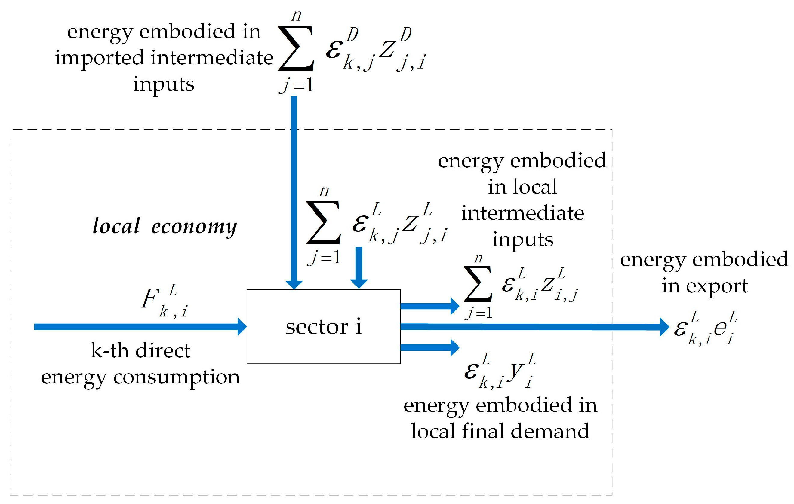
Figure 1 takes sector $i$ as an example, and demonstrates the inflow and outflow relationship for the k-th type of energy in this sector. ${\epsilon }_{k,j}^L$ and ${\epsilon }_{k,j}^D$ represent the EEIs of the k-th type of energy in local sector $j$ and external sector $j$, respectively. According to the material balance theorem, the total amount of embodied energy input should be equal to the total output, such that:

$$F_{k,i}^L+{\displaystyle \sum _{j=1}^n{\epsilon }_{k,j}^L{z}_{j,i}^L+{\displaystyle \sum _{j=1}^n{\epsilon }_{k,j}^D{z}_{j,i}^D={\epsilon }_{k,j}^L({\displaystyle \sum _{j=1}^n{z}_{i,j}^L+y_i^L+e_i^L})}}$$

(1)

For an eco-economic system that contains $n$ sectors and $m$ types of energy, Formula (1) can be expressed as a matrix:

$$F^L+{\epsilon }^L{Z}^L+{\epsilon }^D{Z}^D={\epsilon }^L{X}^L$$

(2)

where $F^L={[F_{k,i}^L]}_{m\times n}$, ${\epsilon }^L={[{\epsilon }_{k,i}^L]}_{m\times n}$, $Z^L={[z_{i,j}^L]}_{n\times n}$, ${\epsilon }^D={[{\epsilon }_{k,i}^D]}_{m\times n}$, ${\epsilon }_{k,i}^D=F_{k,i}^D{(X_i^D)}^{-1}{(I-A^D)}^{-1}$, ${(X_i^D)}^{-1}$ is the inverse matrix of $X_i^D$, ${(I-A^D)}^{-1}$ is the Leontief inverse of the external area, $I$ represents the identity matrix, $A^D=Z^D{(X^D)}^{-1}$, ${\displaystyle \sum _{j=1}^n{z}_{i,j}^L+y_i^L+e_i^L}=X^L$, $X^L={[x_{i,j}^L]}_{n\times n}$, $x_{i,j}=x_i$ when $i=j$, $x_{i,j}=0$ when $i\ne j$; $Z^D={[z_{i,j}^D]}_{n\times n}$, it represents the intermediate input matrix for Beijing in the external region. Beijing’s input–output table is a competitive input–output table; it does not differentiate the proportions of local production and external transfers in the intermediate input. Therefore, in this study, it is assumed that the imported products from other provinces have been distributed to the intermediate input and final use with the same ratio as that of local products [15,44]. This can be calculated by the following formula: $z_{i.j}^D=z_{i.j}^L(\frac{x_i^E}{x_i^L+x_i^E+x_i^M})$, where $x_i^E$ is the domestic transfer input of sector $i$, and $x_i^M$ is the foreign imports of sector $i$. Then, Formula (2) can be changed to:

$${\epsilon }^L=(F^L+{\epsilon }^D{Z}^D){(X^L-Z^L)}^{-1}$$

(3)

After a series of deformations, Formula (3) can also be rewritten as the following to make it easier to understand:

$${\epsilon }^L=(F^L+{\epsilon }^D{Z}^D){(X^L)}^{-1}{(I-A^L)}^{-1}$$

(4)

where $A^L=Z^L{(X^L)}^{-1}$, it is a coefficient matrix that describes the inputs in the production of sectors, ${(I-A^L)}^{-1}$ is the Leontief inverse [45] of the study area, and ${(X^L)}^{-1}$ is the inverse matrix of $X^L$. ${\epsilon }^L$ can be seen as the sum of $F{X}^{-1}{(I-A^L)}^{-1}$ and ${\epsilon }^D{Z}^D{X}^{-1}{(I-A^L)}^{-1}$, where the first term represents the EEI when the external product transfer is not considered, and the second term represents the EEI with the external transfer products embodied.

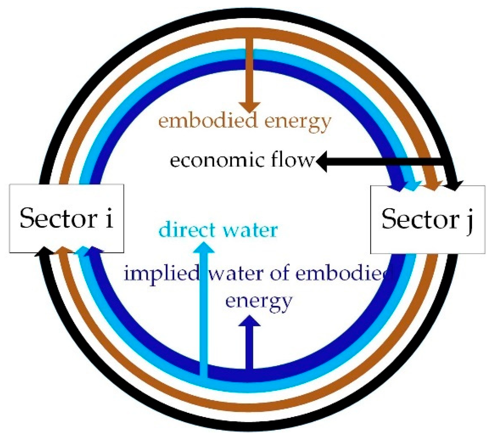
2.2. Water–Energy Relationship Construction

The development of the industrial sector in the economic system requires the consumption of water resources, which is usually measured by direct water use intensity [$W_j=Q_j{/\mathrm{x}}_j$], where $Q_j$ represents the total water consumption of sector $j$, and $x_j$ represents the total input of sector $j$. A larger value of $W_j$ indicates that more water is required per unit of the output product. Excluding water resources, the development of industries also requires the consumption of energy. As mentioned in Section 2.1, these energies may be embodied during local consumption or external import. Regardless of where these energies come from, the water consumed during their production process ultimately serves the regional development of Beijing. At the same time, it is not included in direct water use $Q_j$ and so requires additional consideration. The relationship between these features is illustrated in Figure 2. It can also be understood that water is the ultimate object in this study, which includes direct water use and water use in energy production. The water resources that are consumed in energy production actually serve the sector that the energy ultimately flows into. Therefore, an implied water intensity of embodied energy (IWIEE) is proposed to calculate the water consumption of EEI in the production process. It is obtained by multiplying the embodied energy intensity ${\epsilon }_k^L$ by the water quota $q_k$ for the k-th type of energy; details of $q_k$ in the k-th type of energy can be found in

Table 2. Water quota for various energy processes (m³/tce).

Item	Coal	Coke	Gasoline	Kerosene	Diesel Oil	Fuel Oil	Natural Gas	Electricity
Water quota	0.568	1.904	0.632	0.612	0.570	1.190	1.667	2.441

(more details about $q_k$ can be found in the Supplementary Information in Table S1). The IWIEE of coal, coke, gasoline, kerosene, diesel oil, fuel oil, natural gas, and electricity are calculated, and the sum of the IWIEE of all of the types of energy in sector $j$ is obtained, which is called the implied water intensity of embodied energy in sector $j$, and is denoted by $W_j^E$.

2.3. Complex Network Analysis

2.3.1. Network Construction

In this study, industrial sectors are selected as nodes, implied water flows between sectors are selected as edges, and the flux is utilised as the weight of the edge; all of these parameters are used to build networks. The weight of the edge is determined as follows: $\left(W_j+W_j^E\right)\times z_{i,j}^L$, where $W_j$ represents the direct water use intensity; $W_j^E$ represents the IWIEE; and $z_{i,j}^L$ represents the economic circulation among the industrial sectors. The purpose of this category is to explore network characteristics when direct water consumption, the local IWEE, and the external IWEE are all taken into consideration.

2.3.2. Network Feature Extraction

a. Node strength

Node strength $s_i$ is an indicator that reflects the local information of sector $i$ and is calculated as:

$$s_i={\displaystyle \sum _{j\in N_i}{\omega }_{ij}}$$

(5)

where $N_i$ represents the neighbourhood of sector $i$, and ${\omega }_{ij}$ represents the weight of the edge from node $i$ to node $j$. In directed networks, the node strength can be further divided into in-strength and out-strength, which indicate the amount of implied water flow into and out of the sector, respectively.

b. Average shortest path

In an industry-associated network, the shortest path length represents the minimum number of connections between any two sectors [28]. The average shortest path represents the average shortest path length between any two sectors, and directly reflects the connectivity of the network. The formula is as follows:

$$L=\frac{1}{n(n-1)}{\displaystyle {\sum }_{j=1}^n{\displaystyle \sum _{i=1}^n{d}_{ij}(i\ne j)}}$$

(6)

where $L$ represents the average shortest path, and $d_{ij}$ represents the shortest path length from sector $i$ to sector $j$.

c. Clustering coefficient

The clustering coefficient represents the probability of two sectors that are effectively associated with a certain sector, and are also effectively associated with each other [28]. It can also be described as the probability of “friend’s friends who are also friends”. The formula is as follows:

$$C_i=\frac{E_i}{m_i\times (m_i-1)}$$

(7)

$$C(k)=\frac{1}{n}{\displaystyle \sum _{i=1}^n{C}_i}$$

(8)

where $C_i$ is the clustering coefficient of sector $i$, $m_i$ represents the number of effective links between sector $i$ and other sectors, $m_i\times (m_i-1)$ represents the maximum number of connections that may exist in all of the valid associations of sector $i$, and $E_i$ represents the actual number of connections in all of the valid associations of sector $i$, and is the average clustering coefficient for all of the industrial sectors.

d. Eigenvector centrality

The core principle for eigenvector centrality is that an important node is not only connected to many nodes, but the nodes connected with it are also important nodes [46]. The index assigns values according to the importance of the nodes connected to a specified node, which are determined as follows:

Assuming that $x_v$ represents the weight of node $v$ in the network, $A=(a_{v,t})$ is the adjacency matrix. $a_{v,t}=1$ if an edge exists between node $v$ and $t$; otherwise, $a_{v,t}=0$. The centrality score of node $v$ is defined as:

$$x_v=\frac{1}{\lambda }{\displaystyle \sum _{t\in N(v)}{x}_t=\frac{1}{\lambda }{\displaystyle \sum _{t\in G}{a}_{v,t}{x}_t}}$$

(9)

where $N(v)$ represents the set of nodes connected to node $v$, $\lambda$ is a constant, and $G$ represents a set of nodes in the network. In vector notation, the eigenvector equation can be rewritten as:

$$Ax=\lambda x$$

(10)

Determining eigenvector centrality $x$ can be accomplished by solving these equations. During the actual calculation, an indicator can be calculated directly by the Gephi software (Version 0.9.2, Gephi is a free software which is maintained by Gephi Consortium, details in its homepage https://gephi.org).

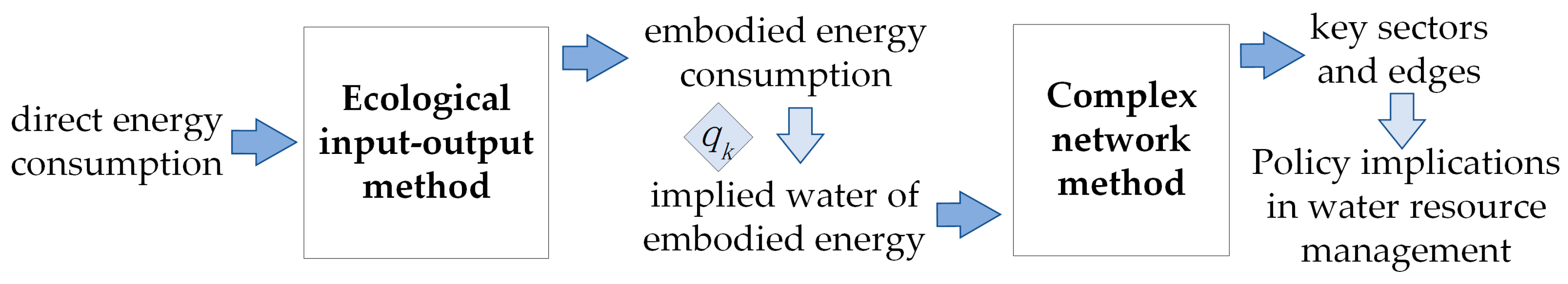
2.4. The Relationship between the Ecological Input–Output Method and Complex Network

The correlation between the ecological input–output method and the complex network in this study is illustrated in Figure 3.

2.5. Data Sources

The data in this study include:

(1)

Input–output data, including China’s input–output table [47] and Beijing’s input–output table [48]. Since there are discrepancies in the division of industrial sectors during these three years, sectors in the input–output table were divided into 40 sectors to maintain a consistent classification (more details can be found in the Supplementary Information, Table S2).

(2)

Energy consumption data, which is derived from the China Energy Statistical Yearbook [49] and the Beijing Statistical Yearbook [50] for the corresponding years. The energy types are divided into coal, coke, gasoline, kerosene, diesel oil, fuel oil, natural gas, and electricity. Limited by the statistical scope of sectoral energy consumption, non-renewable energy such as solar and biomass energy are not included in this article. The sector classification in the Energy Statistical Yearbook is inconsistent with the sectors in the input–output tables; therefore, this study merges and splits sectors in the Energy Statistical Yearbook according to the 40 sectors in the input–output tables, which unifies the energy consumption data.

(3)

Industry water utilisation data from the Beijing Water Resources Bulletin [51], the Beijing Statistical Yearbook [50], and the China Environmental Statistical Yearbook [52], and the related statistics derived from the Beijing Municipal Bureau of Statistics for the corresponding years.

3. Results

3.1. The EEI and IWIEE of Sectors in Beijing

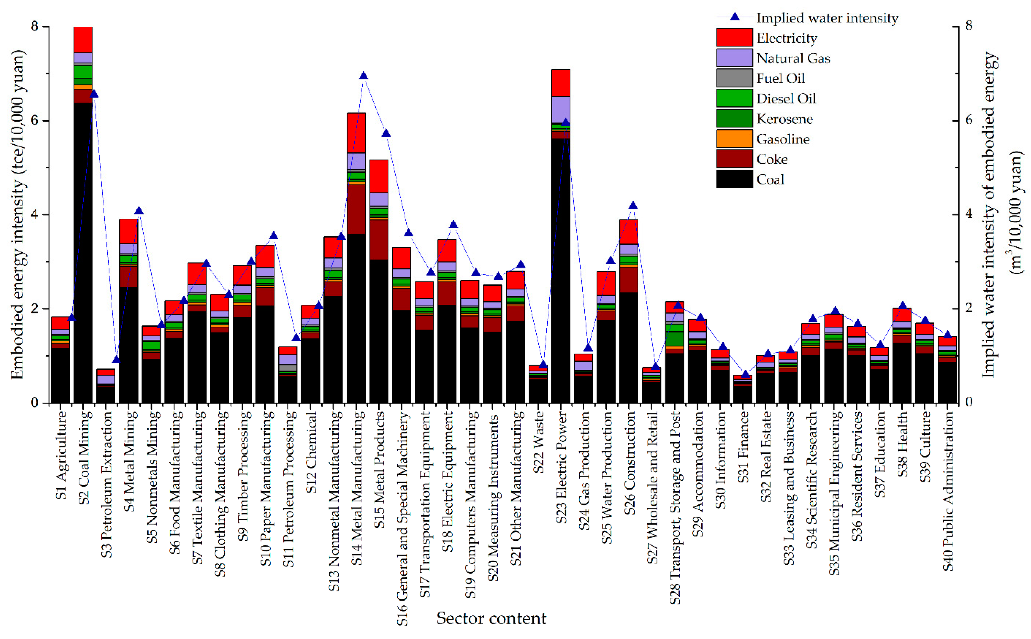
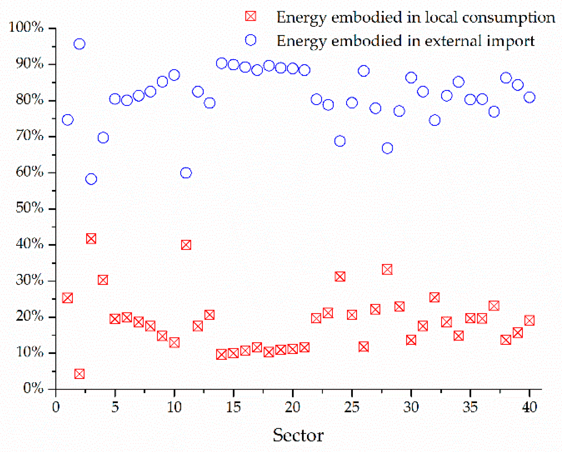
The EEIs of sectors in Beijing in 2012 are illustrated in Figure 4 (only the calculation results for 2012 are shown; the numerical results for all three years are shown in the Supplementary Information in Tables S3–S5). The EEI of specific sectors can reflect the pressure on the environmental system caused by economic activity. Among the 40 sectors in Beijing, the EEI of S2 (coal mining) ranked first (reaching 8.12 tce/10,000 Yuan), followed by S23 (electric power), S14 (metal manufacturing), and S15 (metal products). The sum of the EEI values in these four sectors was almost 30% of the sum of all of the sectors, demonstrating that they are the major energy consumers in Beijing. As shown in Formula (4), there are two sources of energy consumption in the sectors of Beijing. The first source is embodied in local consumption; it is the energy consumption of the sectors that is generated by the internal economic circulation occurring in Beijing, and its percentage is illustrated by blue circles in Figure 5. The second source is embodied in the transfer from other provinces in China; it is the energy consumption generated by the economic circulation among the provinces, and its percentage is shown by red squares in Figure 5. The results show that the EEI embodied in the external transfer is higher than that of the local consumption in each sector. For S2, the EEI embodied in local consumption only accounts for 4.29% of the total—the remaining 95.71% of the EEI comes from external areas. This shows that the coal industry in Beijing is highly dependent on the energy from external provinces. For S23, S14, and S15, the proportions of EEI embodied in local consumption are 21.17%, 9.64%, and 10.73%, respectively. These proportions are higher than that of S2; however, the energy consumption is still primarily based on external transfer.

Some sectors with extremely low direct energy consumption—especially the tertiary industry sectors (S27–S40)—can also obtain a large amount of external energy input through trade, and thus have EEI values that are higher than in some light industry sectors. For example, the EEI of S38 (health) is 2.01 tce/10,000 Yuan, which exceeds the EEI of S22 (waste) of 0.80 tce/10,000 Yuan. Due to energy endowment conditions and environmental factors, local energy production is very limited in Beijing; most of the energy used for final consumption needs to be transferred from external provinces. However, Beijing’s energy efficiency is higher than China’s average. For example, for S2, the energy intensity in China was 4.85 times that of Beijing in 2012. The large amount of energy transfer occurring is equivalent to shifting Beijing’s local energy consumption pressure to outside areas. This approach has solved the energy shortage in Beijing; however, it has also undoubtedly aggravated the pressure on external energy consumption.

On the basis of the EEI values, the IWIEE of each sector was calculated (the calculation results are marked by blue triangles in Figure 4). It can be seen that the change trend of the IWIEE is generally consistent with the EEI. The reason for the subtle difference is that there are differences in water consumption for different types of energy (Table 2). When converting to standard coal, the water consumption per unit of coke is 1.904 m³/tce, which is much higher than that of coal at 0.568 m³/tce. As a result, the IWIEE values of various sectors are not exactly proportional to the corresponding EEIs. From the results, it can be seen that the IWIEE in the tertiary industry sectors are generally lower than those of the secondary industry sectors (S2–S26). Among the 40 sectors, S14 (metal manufacturing) has the largest IWIEE at 6.94 m³/10,000 Yuan. This means that 6.16 tons of standard coal and 6.94 m³ of water is used to produce this energy, and these values are included in the per 10,000 Yuan output. In addition, S2 (coal mining), S23 (electric power), and S15 (metal products) also have large IWIEE values. For these industry sectors, a large amount of water resource will flow into the local area along with energy from outside the area, in order to service local production.

3.2. Implied Water Circulation Network (IWCN) Analysis

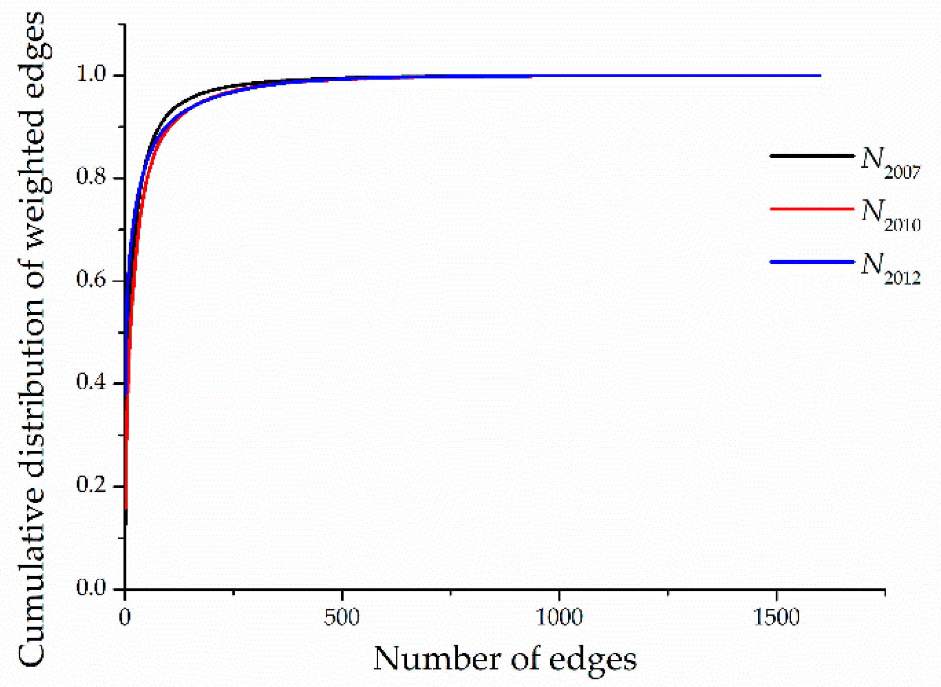
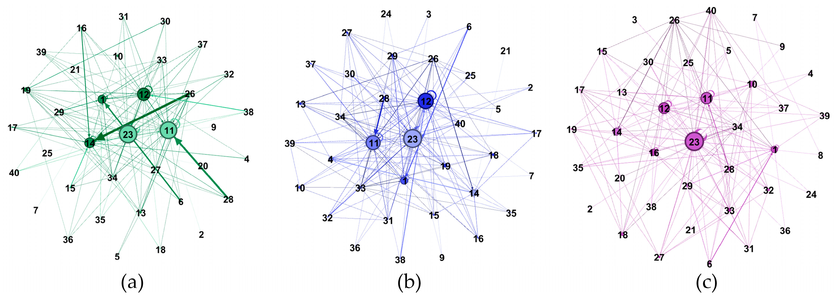
Based on the results in Section 3.1, three networks were constructed based on the Beijing input–output table: N₂₀₀₇, N₂₀₁₀, and N₂₀₁₂ represent the IWCNs in 2007, 2010, and 2012, respectively. It is worth noting that, in order to avoid double counting, when calculating the weights of the edges for the energy industry sectors (S2 coal mining, S3 petroleum extraction, S4 metal mining, S24 gas production), the proportion of the EEI embodied in local consumption is deducted. The cumulative probability distribution of the edges in the network is shown in Figure 6. When the cumulative probability is less than 95%, the cumulative probability increases rapidly with the number of edges. However, when the cumulative probability is greater than 95%, the effect of a greater number of edges on the increase in the cumulative probability becomes very low. This relationship indicates that the main flows in the network occur along a few edges. Therefore, the edges that encompass the weight of the first 95% of the total flow are selected as the edges to build the network. The remaining edges are deleted due to existing in huge numbers, and the small amount of flux. The final networks are shown in Figure 7.

3.2.1. Small-World Networks

Small-world networks are one of the most important features in complex networks. They are networks with a high average clustering coefficient and a low average shortest path [28]. On the one hand, the nodes in the network are closely connected with their neighbouring nodes; on the other hand, only a few nodes are required to reach any other nodes in the network. Most of the nodes in the network are not neighbours of one another. A small-world quotient $[C_{actual}/L_{actual}]\times [L_{random}/C_{random}]$ can be used to test the small-world nature of the network [53]. $C_{actual}$ and $L_{actual}$ refer to the average clustering coefficient and the average shortest path in the actual network, respectively. $C_{random}$ and $L_{random}$ refer to the average clustering coefficient and the average shortest path in a random network of the same size, which are calculated by $d/n$ and $ln(n)/ln(d)$, respectively, and where $n$ represents the number of nodes, and $d$ represents the average degree of all of the nodes. The results are shown in

Table 3. Small-world quotients in each network.

Indicator	N2007	N2010	N2012
Cactual	0.44	0.42	0.37
Lactual	1.66	2.10	1.99
Crandom	0.11	0.13	0.12
Lrandom	2.68	2.28	2.37
Small-world quotient	6.73	3.50	3.62

.

Table 3 presents that the value of $C_{actual}$ floats at around 0.4, which indicates that 40% of the sectors in the IWCN tend to be connected with each other. $L_{random}$ floats at around two, which indicates that only two steps are needed on average for the implied water to flow from one industry sector to another. The small-world quotients in all of the networks are greater than one, indicating that these networks have small-world attributes. A higher clustering coefficient indicates that a triangular relationship is common in the network, and there is no need for excessive intermediation when water flows from one sector to another. This is a useful illustration of the specific small-world property of the IWCN. A lower average shortest path causes the connectivity of the network to improve through the association between sectors. It is worth noting that the small-world nature of the N₂₀₁₀ and N₂₀₁₂ networks is significantly weakened compared with N₂₀₀₇. The reason for this is that, in recent years, the economic exchanges between sectors in Beijing and other provinces in China have become increasingly closed, and as implied water flows more frequently among sectors, this enhances the connectivity and weakens the small-world nature of the network.

3.2.2. Node Strength

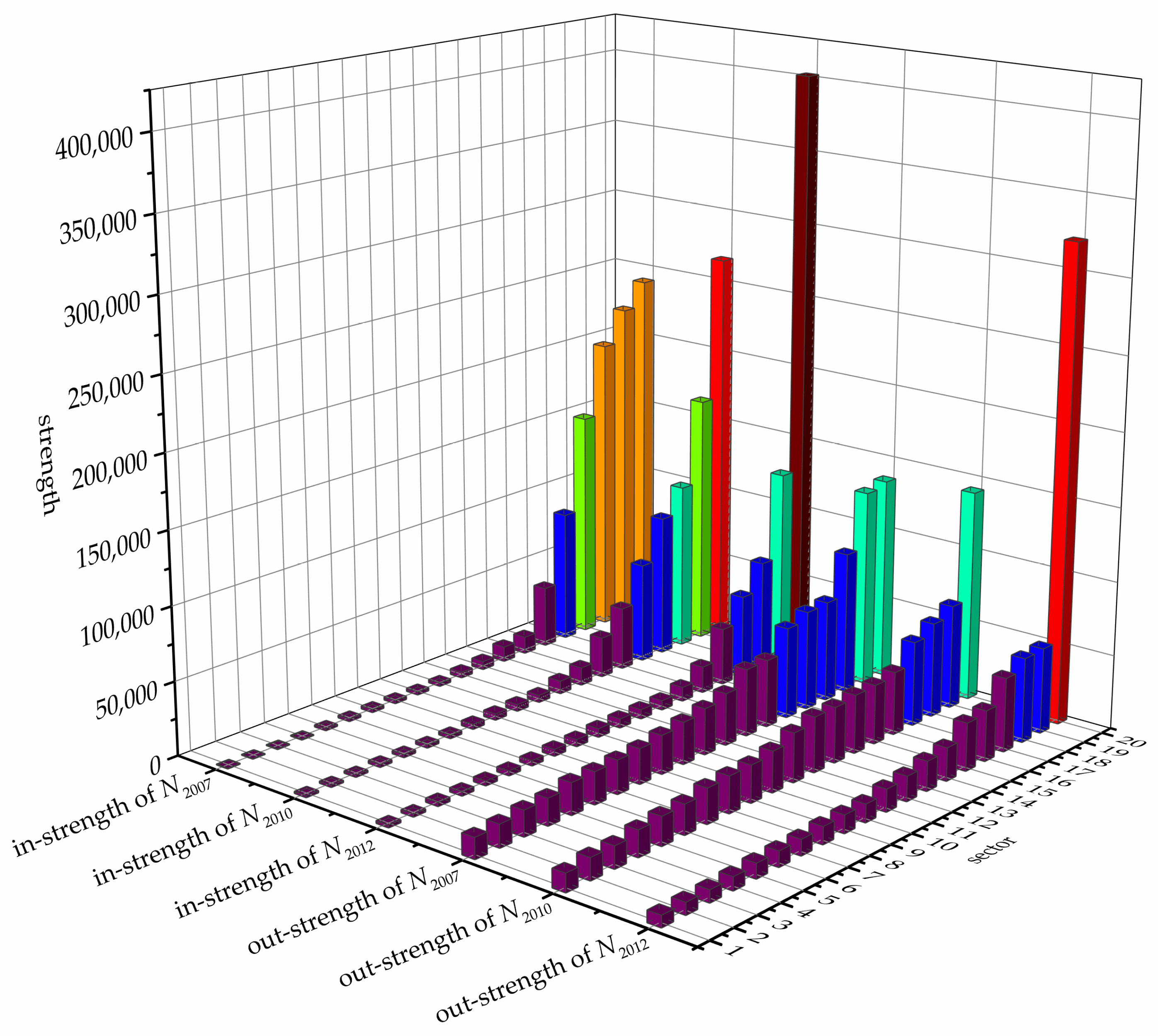
The construction of complex networks helps to identify sectors that have a significant impact on the entire network. One way to measure critical nodes is by using node strength; the greater the strength, the more important the sector tends to be. Utilising the method in a of Section 2.3.2, the in-strength and out-strength of each node in the network are calculated, and the results of the top 20 sectors are shown in Figure 8.

Figure 8 illustrates that there are significant differences among the sectors, regardless of whether the strength type is in-strength or out-strength. The inflow of embodied water is more concentrated in a few sectors with high water intensity, and the sum of the strength of these sectors accounts for the vast majority of the total strength in the network. In contrast, the outflow of embodied water is more evenly distributed among sectors.

Table 4. Top five sectors in each network in terms of strength.

Network	In-Strength	Out-Strength
N2007	S14 Metal Manufacturing (24.05%) S23 Electric Power (22.41%) S11 Petroleum Processing (20.24%) S1 Agriculture (15.45%) S12 Chemical (8.97%)	S26 Construction (13.64%) S23 Electric Power (13.32%) S28 Transport, Storage, and Post (9.60%) S12 Chemical (6.80%) S14 Metal Manufacturing (6.70%)
N2010	S23 Electric Power (31.51%) S11 Petroleum Processing (20.17%) S12 Chemical (13.45%) S1 Agriculture (11.42%) S4 Metal Mining (8.06%)	S23 Electric Power (16.88%) S28 Transport, Storage, and Post (8.31%) S26 Construction (7.56%) S12 Chemical (6.73%) S4 Metal Mining (5.02%)
N2012	S23 Electric Power (50.57%) S1 Agriculture (16.60%) S11 Petroleum Processing (9.38%) S14 Metal Manufacturing (7.05%) S12 Chemical (4.88%)	S23 Electric Power (40.37%) S6 Food Manufacturing (7.27%) S28 Transport, Storage, and Post (7.18%) S26 Construction (6.26%) S29 Accommodation (4.30%)

lists the top five sectors in each network in terms of strength—the numbers in parentheses after the industry number represent the percentage of in-strength (out-strength) to the total value of the in-strength (out-strength) in the corresponding network.

For the in-strength type, the total amount of the top five sectors has always occupied about 90% of the total strength in the three networks. However, the proportions of different sectors have recently undergone major changes. S14 (metal manufacturing) ranked first in 2007, but its rank declined in 2010 and 2012, at which time S23 (electric power) was ranked first. The reason for this change is that although the IWIEE of the S14 sector has increased, the total output value of S14 declined in these years due to the influence of industrial structure adjustment in Beijing. The intermediate input from the other sectors to S14 has also rapidly declined. Therefore, the reduction in intermediate inputs offsets the incremental effect of the increase in the IWIEE; this made the in-strength of S14 fall rapidly during the study period. For S23, the direct water consumption significantly increased, and the input from the other sectors into S23 also increased with the gradual improvement of living standards. In addition, the IWIEE of this sector has increased. A combination of these three factors has resulted in a significant increase in the in-strength of S23. In addition to these two sectors, S11 (petroleum processing), S1 (agriculture), and S12 (chemical) also have large in-strengths, which reflect a high level of potential water consumption.

For the out-strength, the total amount of the top five sectors accounted for about 50% of the total strength (rising to 65% in 2012). Similar to the in-strength, the proportions of different sectors have undergone major changes. For example, S23 (electric power) still occupies a dominant position, and its status is increasingly important: its out-strength had reached 40% of the total as of 2012. This sector not only consumes a large amount of water resources, but also exports products containing a large amount of implied water and serves the production activities of other sectors, which makes it a key node in the network. The ranking of S26 (construction) declined, which was mainly attributable to the decline in the IWIEE. The out-strength values in S28 (transport, storage, and post), S12 (chemical), and S6 (food manufacturing) are also relatively large, reflecting a strong water supply capacity.

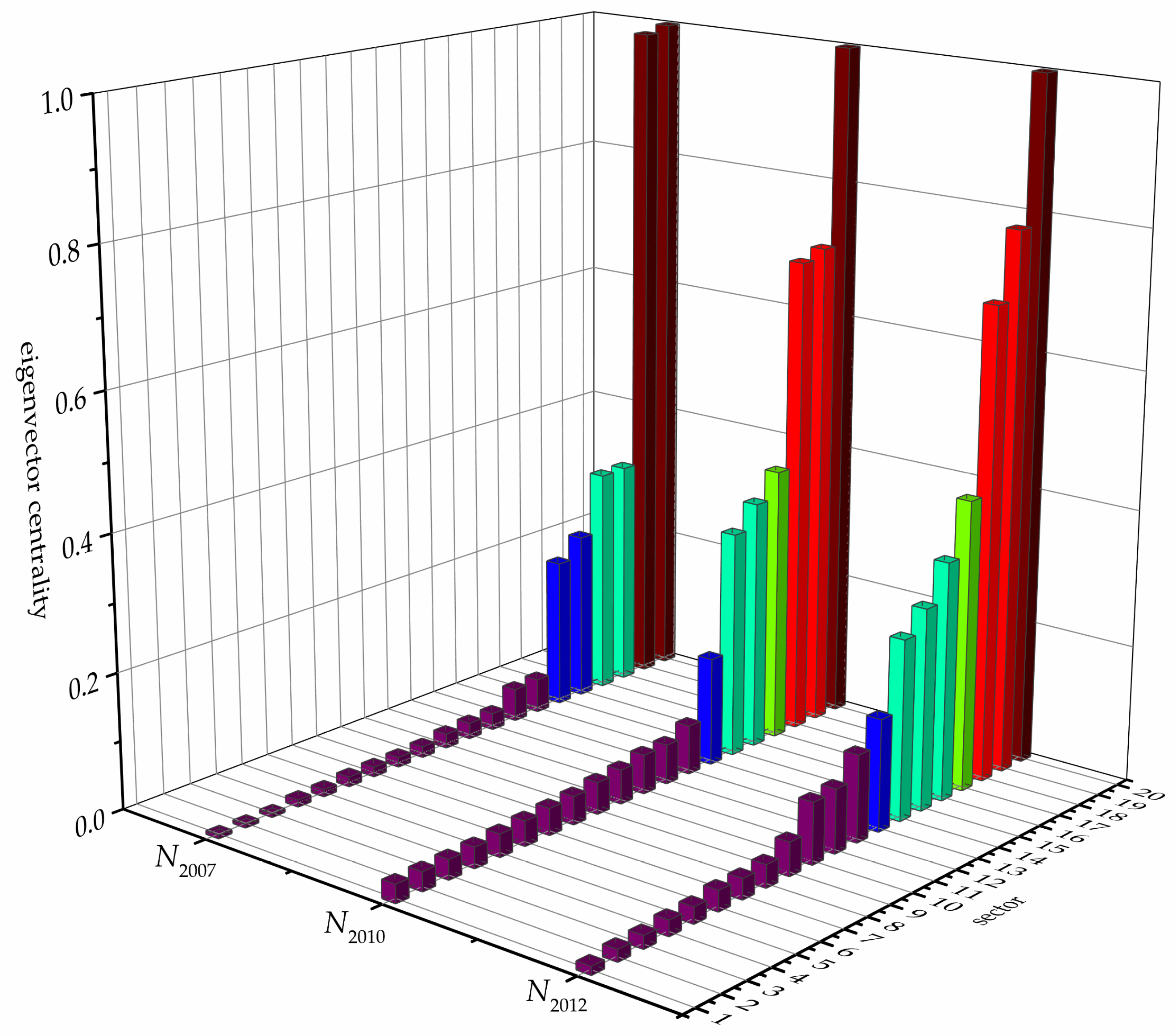
3.2.3. Eigenvector Centrality

In IWCNs, sectors with high in-strength or out-strength values are regarded as key sectors. In addition, the importance of nodes is closely related to the importance of the nodes that they are connected to. Eigenvector centrality is a key indicator to measure this property, as it represents important nodes that are connected to many other nodes, and posits that the nodes that are connected to these nodes are also important nodes. The calculation results of the top 20 sectors are shown in Figure 9. Sectors with a large eigenvector centrality only account for a small proportion of the total number of sectors, which is consistent with the objective fact that sectors with high strength only occupy a small proportion of all of the sectors.

Table 5. Sectors with relatively large eigenvector centrality values.

Sector Number and Eigenvector Centrality
N2007	S23	S11
	1.00	0.99
N2010	S23	S12	S11	S4
	1.00	0.72	0.70	0.40
N2012	S23	S11	S12	S14
	1.00	0.79	0.69	0.43

lists the sectors with relatively large eigenvector centrality values. Among these sectors, S23 (electric power) has the largest eigenvector centrality (i.e., one across the three networks). This means that all of the sectors connected to S23 are sectors with large node strengths, which is consistent with S23 providing basic energy, such as electricity, which is needed by the other sectors to maintain normal production. In addition, S11 (petroleum processing), S12 (chemical), S14 (metal manufacturing), and S4 (metal mining) also have relatively large eigenvector centrality values, which indicate that these are also key sectors. A change in the input or output relationship significantly affects important sectors that are associated with sectors that have large eigenvector centralities.

3.2.4. Key Indirect Water Flow Paths

The analyses of node strength and eigenvector centrality are based on key nodes, and the research below will be mainly focussed on edges that carry large amounts of implied water. In N₂₀₀₇, the top 40 weights (2.50% of the total number of edges) occupy 80% of the total network flow. The edges with the top three weights are listed in

Table 6. Edges with the top three weights in each network.

Network	Source	Target
N2007	S23 Electric Power S26 Construction S28 Transport, Storage, and Post	S23 Electric Power S14 Metal Manufacturing S11 Petroleum Processing
N2010	S23 Electric Power S28 Transport, Storage, and Post S6 Food Manufacturing	S23 Electric Power S11 Petroleum Processing S1 Agriculture
N2012	S23 Electric Power S6 Food Manufacturing S28 Transport, Storage, and Post	S23 Electric Power S1 Agriculture S11 Petroleum Processing

. The sum of the weights for these three edges was more than 30% of the total weight, indicating that they are the most important edges in the network. In N₂₀₁₀, the top 50 weights (3.13% of the total number of edges) occupy 80% of the total network flow. Among them, the edges with the top three weights are also listed in Table 6. The sum of the weights for these three edges was 26.19% of the total weight. In N₂₀₁₂, the top 40 weights (2.50% of the total number of edges) occupy 80% of the total network flow. Among them, the sum of the weights for the top three edges was more than half of the total weight. Compared with N₂₀₀₇ and N₂₀₁₀, water flow is more concentrated in a few key edges in N₂₀₁₂, and the heterogeneity of the network is more significant. Therefore, the identification of key edges plays an important role in improving network properties, and is also the basis for proposing water-saving countermeasures. Note that S23 (electric power) → S23 is a “self-loop” in which the implied water exported by the sector is reinvested in the production in this sector. The products of S23 are electricity and heat; however, the process of generating electricity and heat still requires the consumption of electricity and heat to maintain normal production processes. Water, energy, and energy-implied water are all consumed in this process, which is why the “self-loop” appears in the calculation result.

In the network, the edges between nodes can be connected by different path lengths, and the contributions of different paths are different in each network. The method used by Sun [27] was referenced, and the appropriate changes were made to measure the key paths in the network. The concrete steps are as follows: (1) all of the nodes in the network are identified as initial nodes for constructing key paths; (2) the edge with the largest weight among all of the edges that are connected to the initial node is selected (excluding the node itself), and the target node of this edge is used as the second node in the key path; (3) the second step is repeated until the last node returns to the penultimate node, and the key path search is completed; and (4) the sum of the weights for the edges in each key path is calculated, and the top five key paths are selected as the final key paths. The key paths in the three networks are listed in

Table 7. Key paths in the three networks.

Network	Source
N2007	S26 (Construction)→S14 (Metal Manufacturing)→S11 (Petroleum Processing)→S23 (Electric Power) S28 (Transport, Storage, and Post)→S11 (Petroleum Processing)→S23 (Electric Power) S6 (Food Manufacturing)→S1 (Agriculture)→S11 (Petroleum Processing)→S23 (Electric Power) S38 (Health)→S12 (Chemical)→S11 (Petroleum Processing)→S23 (Electric Power) S30 (Information)→S19 (Computers Manufacturing)→S12 (Chemical)→S11 (Petroleum Processing)→S23 (Electric Power)
N2010	S14 (Metal Manufacturing)→S4 (Metal Mining)→S11 (Petroleum Processing)→S23 (Electric Power) S38 (Health)→S12 (Chemical)→S11 (Petroleum Processing)→S23 (Electric Power) S34 (Scientific Research)→S12 (Chemical)→S11 (Petroleum Processing)→S23 (Electric Power) S19 (Computers Manufacturing)→S12 (Chemical)→S11 (Petroleum Processing)→S23 (Electric Power) S17 (Transportation Equipment)→S12 (Chemical)→S11 (Petroleum Processing)→S23 (Electric Power)
N2012	S6 (Food Manufacturing)→S1 (Agriculture)→S23 (Electric Power)→S11 (Petroleum Processing) S2 (Coal Mining)→S28 (Transport, Storage and Post)→S11 (Petroleum Processing)→S23 (Electric Power) S28 (Transport, Storage, and Post)→S11 (Petroleum Processing)→S23 (Electric Power) S26 (Construction)→S14 (Metal Manufacturing)→S23 (Electric Power)→S11 (Petroleum Processing) S29 (Accommodation)→S1 (Agriculture)→S23 (Electric Power)→S11 (Petroleum Processing)

. The results represent that there are always between three and five nodes in the key paths of the three networks, indicating that the main water flow is always concentrated in a few sectors in IWCNs. This property has not changed much over time. In addition, all of the key paths are terminated at S11 (or S23), and the penultimate sector is always S23 (or S11). This also illustrates the important role of S11 and S23 in the network from another perspective. The water circulation relationship is very close between these two sectors, and between these two sectors and others.

4. Discussion

The energy consumption of all of the sectors in Beijing is mainly embodied in the transfer of the external provinces of China. The proportion embodied in local consumption is low, which is primarily due to the constraints of resource endowment conditions and the influence of environmental protection policies in the capital area. The IWIEE is defined as the water consumption during energy production, and is calculated by multiplying the EEI by water consumption per unit of energy. Therefore, the variation trend of the IWIEE is consistent with that of the EEI. The implied water networks (with 40 nodes) were built based on the IWIEE and direct water consumption. The results show that these networks have small-world network characteristics, and a change in key nodes significantly influences the function of the whole system [27]. Fluctuations in key nodes quickly spread across the entire network, which may have positive or negative effects. A positive effect is that the water-saving caused by regulated water use in key sectors will quickly spread to other sectors, promoting water conservation for the entire economic system. A potential negative effect is that when there is a water shortage in key nodes, the small-world network characteristics mean that this effect also quickly spreads to other sectors. In other words, it directly or indirectly affects the water security of other sectors, and thus poses a potential threat to regional economic development. Node strength, eigenvector centrality, key edges, and key paths are further selected as indicators to measure key sectors and edges in the network.

This study combines the ecological input–output method with a complex network model, and preliminarily explores the implied water circulation characteristics from the perspective of embodied energy. Several shortcomings and corresponding directions for future research are relevant to this research. First, regarding the relationship between water and energy, this study focussed on water consumption during energy processes. Bidirectionally accounting for these two features could be further explored in future research to achieve collaborative research regarding the energy–water relationship. Second, due to limited access to external data when calculating the EEI, only the economic flow among the provinces in China was taken into consideration. The impact from other countries on the EEI is not considered; therefore, the EEI may be underestimated. In the future, the calculation of the EEI could be improved by improved access to external data. Third, sensitivity analysis is not considered in this article. In IWCNs, finding the energy consumption type or direct water use sector that has a significant impact on the network characteristics is helpful to find better water-saving optimisation solutions, so sensitivity analysis could bring more practical benefits to the comprehensive management of regional water resources utilisation, and would be a direction for further research. Finally, the energy production water quota was used to calculate the IWEE; however, the water quota is a fixed value, and interannual variations may be caused by technological improvements, policy controls, and other factors that have not been considered in this paper, which may also bias the results. In the future, life cycles and other methods could be used to calculate water consumption during energy processes more accurately.

5. Conclusions

The embodied energy intensity (EEI) and implied water intensity of embodied energy (IWIEE) were calculated and analysed in this paper; then, implied water circulation networks (IWCNs) for 40 sectors in the years 2007, 2010, and 2012 in Beijing were constructed. The results indicate that the energy consumption of all of the sectors is mainly embodied in the transfer of external provinces of China. Some tertiary industry sectors with low direct energy consumption also have high EEI values benefiting from economic circulation. The variation trend of the IWIEE is consistent with the EEI. The IWCN has small-world characteristics, and shows a weakening trend. The node strength, eigenvector centrality, key edge, and key path were selected as indicators to measure key sectors and edges in the network. Finally, water-saving measures and suggestions were proposed according to the calculation results of the complex network characteristics. The coupled utilisation of the ecological input–output method and complex network method provide the possibility of combining multi-scale embodied energy with structural system characteristics analysis, and further provide new ideas for regional water resource management from the perspective of energy consumption.

Policy Implications

IWCNs with small-world network characteristics are sensitive and vulnerable, and the most important implication of this for policy management is that water use changes in key nodes will have a systematic impact on the entire IWCN. Therefore, it is of vital importance to identify key nodes and undertake appropriate countermeasures to improve the properties of IWCNs.

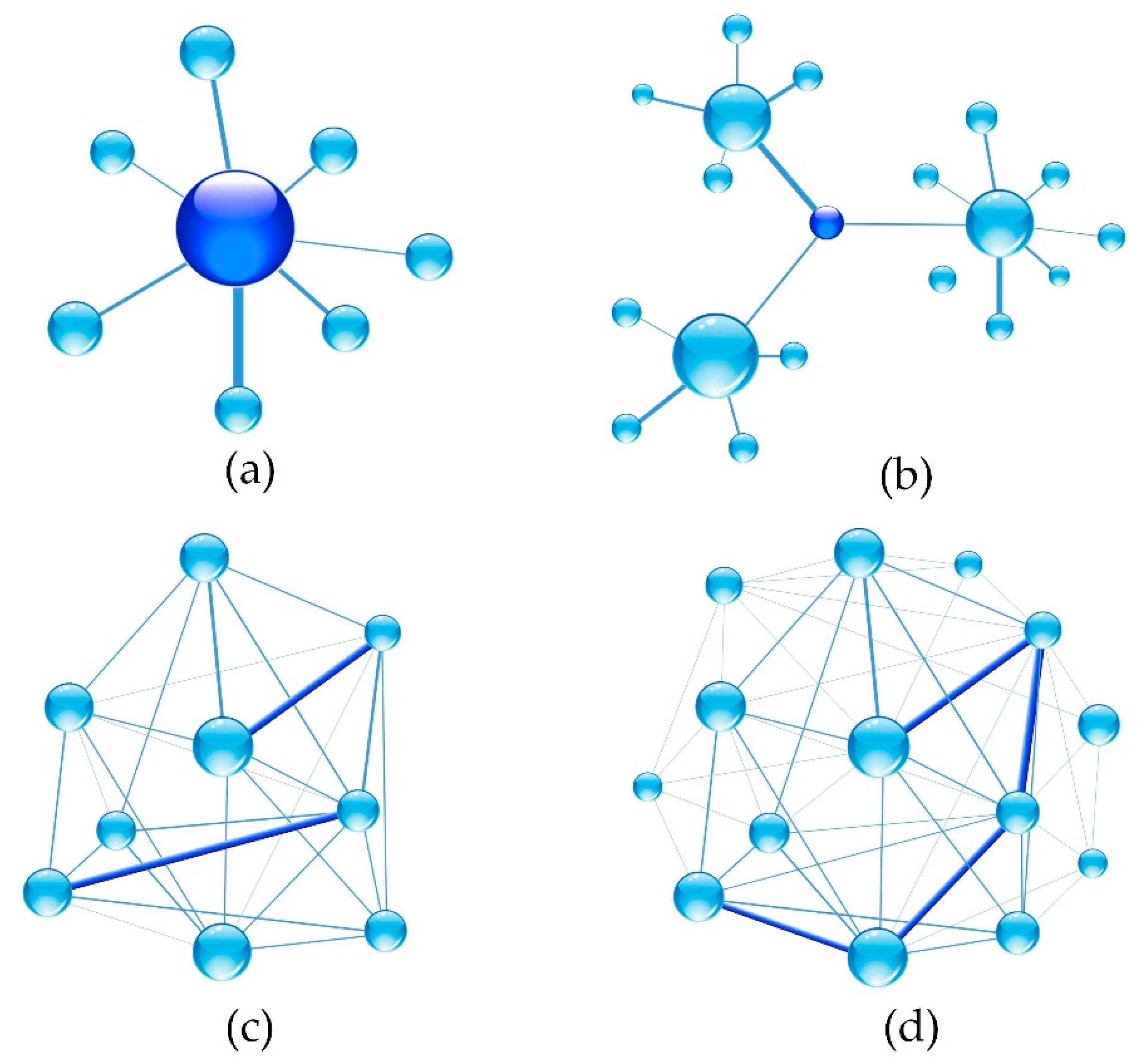
The nodes with high strength values can be regarded as key nodes in the network (as shown in Figure 10a). A large amount of implied water flows into or out of these sectors, and they occupy large proportions of entire IWCNs. Therefore, if such sectors are properly regulated, the total flux of the entire IWCN will be effectively reduced. This has notable implications for water-saving policy formulation. First, for nodes with high strength values, the energy use that occurs with a large unit of water consumption (such as in coke) should be reduced, and energy sources with low water consumption requirements should be used as materials for production. Second, policies should be focussed on improving the direct water use efficiency, and if necessary, increasing the water price of these sectors to limit water consumption. Third, it is necessary to strengthen the economic exchange between these sectors and their upstream sectors with a lower IWIEE. This approach will stimulate sectors with a high out-strength to increase their water use efficiency, and use less water-intensive energy sources as production materials, thus forming a virtuous circle in IWCNs.

Nodes with large eigenvector centrality values can also be seen as the key nodes in the network (as shown in Figure 10b). Unlike nodes with high strength values, there may be not a large amount of implied water flowing into or out of these sectors. However, they are connected to high strength nodes. Therefore, they can be involved in the management of water-saving policies by improving the direct water use efficiency and compressing water supply in these sectors to a moderate degree, which will significantly affect the water usage in the key sectors that are connected to them.

In addition, the determination of key edges and key paths has also contributed to new ideas in water resource management. In IWCNs, very few edges occupy a large proportion of the entire circulation network (as shown in Figure 10c), indicating that the implied water circulation can be significantly affected through the regulation of economic circulation in key edges, or by replacing the upstream sector of the target node in the key edge with sectors with a low IWIEE. Key paths can be regarded as special connectors to key edges in the network (as shown in Figure 10d), and they represent the dominant water resource circulation path in the network. Therefore, blocking or replacing the appropriate edges in the key path will also change the circulation characteristics for the whole key path, which will affect the entire implicit water circulation system.

It should be noted that “water-saving” in this study actually includes both water-saving and energy-saving, because the IWEE is calculated based on energy consumption. Therefore, “water-saving” includes both the saving of natural water resources and the choosing of energy processes with relatively low water consumption, in order to achieve comprehensive water-saving.

References

- Ye, Q.; Li, Y.; Zhuo, L.; Zhang, W.; Xiong, W.; Wang, C.; Wang, P. Optimal allocation of physical water resources integrated with virtual water trade in water scarce regions: A case study for Beijing, China. Water Res. 2018, 129, 264–276. [Google Scholar] [CrossRef] [PubMed]
- Dalin, C.; Hanasaki, N.; Qiu, H.; Mauzerall, D.L.; Rodrigueziturbe, I. Water resources transfers through Chinese interprovincial and foreign food trade. Proc. Natl. Acad. Sci. USA 2014, 111, 9774–9779. [Google Scholar] [CrossRef] [PubMed] [Green Version]
- Avrin, A.P.; He, G.; Kammen, D.M. Assessing the impacts of nuclear desalination and geoengineering to address China’s water shortages. Desalination 2015, 360, 1–7. [Google Scholar] [CrossRef]
- Li, H.; Mu, H.; Zhang, M. Analysis of China’s energy consumption impact factors. Procedia Environ. Sci. 2011, 11, 824–830. [Google Scholar] [CrossRef]
- National Bureau of Statistics (NSB). China Energy Statistical Yearbook 2017; China Statistics Press: Beijing, China, 2018. (In Chinese)
- Liu, X.; Zhou, D.; Zhou, P.; Wang, Q. Factors driving energy consumption in China: A joint decomposition approach. J. Clean. Prod. 2017, 172, 724–734. [Google Scholar] [CrossRef]
- Cellura, M.; Longo, S.; Mistretta, M. The energy and environmental impacts of Italian households consumptions: An input–output approach. Renew. Sustain. Energy Rev. 2011, 15, 3897–3908. [Google Scholar] [CrossRef]
- Li, H.; Liu, G.; Yang, Z.; Hao, Y. Urban gray water footprint analysis based on input-output approach. Energy Procedia 2016, 104, 118–122. [Google Scholar] [CrossRef]
- Kucukvar, M.; Egilmez, G.; Tatari, O. Sustainability assessment of U.S. final consumption and investments: Triple-bottom-line input–output analysis. J. Clean. Prod. 2014, 81, 234–243. [Google Scholar] [CrossRef]
- Kuhtz, S.; Zhou, C.; Albino, V.; Yazan, D.M. Energy use in two Italian and Chinese tile manufacturers: A comparison using an enterprise input–output model. Energy 2010, 35, 364–374. [Google Scholar] [CrossRef]
- Chen, G.; Chen, Z. Greenhouse gas emissions and natural resources use by the world economy: Ecological input–output modeling. Ecol. Model. 2011, 222, 2362–2376. [Google Scholar] [CrossRef]
- Shao, L. Multi-Scale Input-Output Analysis of Embodied Water and Its Engineering Applicatons; Peking University: Beijing, China, 2014. [Google Scholar]
- Chen, G.; Chen, H.; Chen, Z.; Zhang, B.; Shao, L.; Guo, S.; Zhou, S.; Jiang, M. Low-carbon building assessment and multi-scale input–output analysis. Commun. Nonlinear Sci. Numer. Simul. 2011, 16, 583–595. [Google Scholar] [CrossRef]
- Zhou, S.; Chen, H.; Li, S. Resources use and greenhouse gas emissions in urban economy: Ecological input–output modeling for Beijing 2002. Commun. Nonlinear Sci. Numer. Simul. 2010, 15, 3201–3231. [Google Scholar] [CrossRef]
- Shao, L.; Guan, D.; Wu, Z.; Wang, P.; Chen, G. Multi-scale input-output analysis of consumption-based water resources: Method and application. J. Clean. Prod. 2017, 164, 338–346. [Google Scholar] [CrossRef]
- Liu, S.; Wu, X.; Han, M.; Zhang, J.; Chen, B.; Wu, X.; Wei, W.; Li, Z. A three-scale input-output analysis of water use in a regional economy: Hebei province in China. J. Clean. Prod. 2017, 156, 962–974. [Google Scholar] [CrossRef]
- Chen, G.; Wu, X. Energy overview for globalized world economy: Source, supply chain and sink. Renew. Sustain. Energy Rev. 2017, 69, 735–749. [Google Scholar] [CrossRef]
- Wu, X.; Xia, X.; Chen, G.; Wu, X.; Chen, B. Embodied energy analysis for coal-based power generation system-highlighting the role of indirect energy cost. Appl. Energy 2016, 184, 936–950. [Google Scholar] [CrossRef]
- Sun, X.; An, H. Emergy network analysis of Chinese sectoral ecological sustainability. J. Clean. Prod. 2017, 174, 548–559. [Google Scholar] [CrossRef]
- Zhang, L.; Hao, Y.; Chang, Y.; Pang, M.; Tang, S. Emergy based resource intensities of industry sectors in China. J. Clean. Prod. 2017, 142, 829–836. [Google Scholar] [CrossRef]
- Chen, Z.; Chen, G.; Chen, B. Embodied carbon dioxide emissions of the world economy: A systems input-output simulation for 2004. Procedia Environ. Sci. 2010, 2, 1827–1840. [Google Scholar] [CrossRef]
- Chen, Z.; Chen, G. Virtual water accounting for the globalized world economy: National water footprint and international virtual water trade. Ecol. Indic. 2013, 28, 142–149. [Google Scholar] [CrossRef]
- Chen, G.; Chen, Z. Carbon emissions and resources use by Chinese economy 2007: A 135-sector inventory and input–output embodiment. Commun. Nonlinear Sci. Numer. Simul. 2010, 15, 3647–3732. [Google Scholar] [CrossRef]
- Chen, Z.; Chen, G.; Zhou, J.; Jiang, M.; Chen, B. Ecological input–output modeling for embodied resources and emissions in Chinese economy 2005. Commun. Nonlinear Sci. Numer. Simul. 2010, 15, 1942–1965. [Google Scholar] [CrossRef]
- Chen, G.; Bo, Z. Greenhouse gas emissions in China 2007: Inventory and input–output analysis. Energy Policy 2010, 38, 6180–6193. [Google Scholar] [CrossRef]
- Li, J.; Chen, G.; Wu, X.; Hayat, T.; Alsaedi, A.; Ahmad, B. Embodied energy assessment for Macao's external trade. Renew. Sustain. Energy Rev. 2014, 34, 642–653. [Google Scholar] [CrossRef]
- Sun, X.; An, H.; Gao, X.; Jia, X.; Liu, X. Indirect energy flow between industrial sectors in China: A complex network approach. Energy 2016, 94, 195–205. [Google Scholar] [CrossRef]
- Watts, D.J.; Strogatz, S.H. Collective dynamics of “small-world” networks. Nature 1998, 393, 440. [Google Scholar] [CrossRef] [PubMed]
- Barabasi, A.L.; Albert, R. Emergence of scaling in random networks. Science 1999, 286, 509–512. [Google Scholar] [PubMed]
- Newman, M.E.J. The structure and function of complex networks. SIAM Rev. 2003, 45, 167–256. [Google Scholar] [CrossRef]
- Sartori, M.; Fracasso, A.; Riccaboni, M.; Schiavo, S. Modeling the future evolution of the virtual water trade network: A combination of network and gravity models. Adv. Water Resour. 2017, 538–548. [Google Scholar] [CrossRef]
- Du, R.; Wang, Y.; Dong, G.; Tian, L.; Liu, Y.; Wang, M.; Fang, G. A complex network perspective on interrelations and evolution features of international oil trade, 2002–2013. Appl. Energy 2017, 196, 142–151. [Google Scholar] [CrossRef]
- Yang, Y.; Poon, J.P.H.; Liu, Y.; Bagchi-Sen, S. Small and flat worlds: A complex network analysis of international trade in crude oil. Energy 2015, 93, 534–543. [Google Scholar] [CrossRef] [Green Version]
- Zhong, W.; An, H.; Gao, X.; Sun, X. The evolution of communities in the international oil trade network. Physica A 2014, 413, 42–52. [Google Scholar] [CrossRef]
- Chen, Z.; An, H.; Gao, X.; Li, H.; Hao, X. Competition pattern of the global liquefied natural gas (LNG) trade by network analysis. J. Nat. Gas Sci. Eng. 2016, 33, 769–776. [Google Scholar] [CrossRef]
- Geng, J.; Ji, Q.; Fan, Y. A dynamic analysis on global natural gas trade network. Appl. Energy 2014, 132, 23–33. [Google Scholar] [CrossRef]
- Gao, C.; Sun, M.; Shen, B. Features and evolution of international fossil energy trade relationships: A weighted multilayer network analysis. Appl. Energy 2015, 156, 542–554. [Google Scholar] [CrossRef]
- Hao, X.; An, H.; Qi, H.; Gao, X. Evolution of the exergy flow network embodied in the global fossil energy trade: Based on complex network. Appl. Energy 2016, 162, 1515–1522. [Google Scholar] [CrossRef]
- Chen, B.; Li, J.; Wu, X.; Han, M.; Zeng, L.; Li, Z.; Chen, G.Q. Global energy flows embodied in international trade: A combination of environmentally extended input–output analysis and complex network analysis. Appl. Energy 2018, 210, 98–107. [Google Scholar] [CrossRef]
- An, Q.; An, H.; Wang, L.; Gao, X.; Lv, N. Analysis of embodied exergy flow between Chinese industries based on network theory. Ecol. Model. 2015, 318, 26–35. [Google Scholar] [CrossRef]
- Wang, X.; Wei, W.; Ge, J.; Wu, B.; Bu, W.; Li, J.; Yao, M.; Guan, Q. Embodied rare earths flow between industrial sectors in China: A complex network approach. Resour. Conserv. Recycl. 2017, 125, 363–374. [Google Scholar] [CrossRef]
- Beijing Municipal Water Affairs Bureau. Beijing Municipal Water Affairs Bureau 2016; Beijing Municipal Water Affairs Bureau: Beijing, China, 2016. (In Chinese)
- Sun, C.; Ma, T.; Xu, M. Exploring the prospects of cooperation in the manufacturing industries between India and China: A perspective of embodied energy in India-China trade. Energy Policy 2018, 113, 643–650. [Google Scholar] [CrossRef]
- Shao, L.; Chen, G. Embodied water accounting and renewability assessment for ecological wastewater treatment. J. Clean. Prod. 2016, 112, 4628–4635. [Google Scholar] [CrossRef]
- Miller, R.E.; Blair, P.D. Input-Output Analysis: Foundations and Extensions; Cambridge University Press: Cambridge, UK, 1985; pp. 1293–1304. [Google Scholar]
- Parand, F.A.; Rahimi, H.; Gorzin, M. Combining fuzzy logic and eigenvector centrality measure in social network analysis. Physica A 2016, 459, 24–31. [Google Scholar] [CrossRef]
- National Bureau of Statistics (NSB). Input-Output Table of China Economy in 2007, 2010, 2012; China Statistical Publishing House: Beijing, China, 2009, 2012, 2014. Available online: http://www.stats.gov.cn/english/Statisticaldata/AnnualData/ (accessed on 22 June 2018).
- Beijing Statistical Bureau (BSB). Input-Output Table of Beijing Economy in 2007, 2010, 2012; China Statistical Publishing House: Beijing, China, 2009, 2012, 2014. Available online: http://www.bjstats.gov.cn/English/ (accessed on 22 June 2018).
- National Bureau of Statistics (NSB). China Energy Statistical Yearbook 2007, 2010, 2012; China Statistics Press: Beijing, China, 2008, 2011, 2013. (In Chinese)
- Beijing Statistical Bureau (BSB). Beijing Statistical Yearbook 2007, 2010, 2012; China Statistics Press: Beijing, China, 2008, 2011, 2013. (In Chinese)
- Beijing Municipal Water Affairs Bureau. Beijing Municipal Water Affairs Bureau 2007, 2010, 2012; Beijing Municipal Water Affairs Bureau: Beijing, China, 2008, 2011, 2013. (In Chinese)
- National Bureau of Statistics (NSB). China Environmental Statistical Yearbook 2007, 2010, 2012; 2008, 2011, 2013. (In Chinese)
- Davis, G.F.; Yoo, M.; Baker, W.E. The small world of the american corporate elite, 1982–2001. Strateg. Organ. 2003, 1, 301–326. [Google Scholar] [CrossRef]
Figure 1.
The embodied energy balance of sector in an economic system (with the k-th type of energy).
Figure 2.
In the national economic system, economic, energy, and water flows exist among most of the sectors. A brief description is given in this figure for sectors and . The circulation of products or services between sectors and is called the economic flow. Water resources directly consumed by the industrial sector circulate among sectors via products or services; this is called direct water flow. Industrial development also requires the consumption of energy, which may derive from local production or external inputs, and is called embodied energy. Energy consumed in the industrial sector also requires water during the production process; these potential water resources also circulate among the various sectors by means of products or services, and are referred to as the IWEE. Combining direct water flow with the IWEE means considering the water consumption of energy based on direct water use, and exploring the water flow characteristics among the sectors.
Figure 3.
Flow diagram of the ecological input–output method and the complex network. Direct energy consumption is the input data for the ecological input–output method, and embodied energy consumption is obtained by calculation. Further, the implied water of embodied energy is calculated by multiplying the embodied energy consumption by , and then is input into the calculation of complex network indicators. Finally, key sectors and edges are identified by complex network characteristics to better implement water resource management.
Figure 4.
Embodied energy intensity (EEI) and implied water intensity of embodied energy (IWIEE) values of sectors in Beijing in 2012. The abscissa shows 40 sectors in Beijing; the names of the sectors are expressed in abbreviations, and the full names of these sectors are shown in Table S2 in the Supplementary Information. The left ordinate shows EEI, and the unit is tce/1000 Yuan. The right ordinate shows IWIEE, and the unit is m3/10,000 Yuan.
Figure 5.
Proportion of the EEI embodied in local consumption and external transfer in 2012.
Figure 6.
Cumulative probability distribution of the weighted edges. The abscissa is the number of edges in the network, and the ordinate is the cumulative probability of the weighted edges sorted in descending order.
Figure 7.
(a–c) represent the implied water circulation network (IWCN) in 2007, 2010, and 2012, respectively. The size of the node represents the implied water flow into the node; the larger the node, the larger the value. The colour intensity represents the implied water flow out of the node; the darker the colour, the greater the value.
Figure 8.
Top 20 sectors in each network in terms of strength. The order of the networks from left to right is the in-strength of 2007, 2010, and 2012, and the out-strength of 2007, 2010, and 2012, respectively.
Figure 9.
Top 20 sectors in each network in terms of eigenvector centrality values.
Figure 10.
Schematic of key nodes and key edges in the network. (a–d) represent the key node, the node with a large eigenvector centrality value, the key edge, and the key path, respectively.