Transmission of Water Waves under Multiple Vertical Thin Plates


1
College of Shipbuilding Engineering, Harbin Engineering University, Harbin 150001, China
2
School of Engineering and Mathematical Sciences, City University London, London EC1V 0HB, UK
*
Author to whom correspondence should be addressed.
Water 2018, 10(4), 517; https://doi.org/10.3390/w10040517
Submission received: 17 March 2018
/
Revised: 6 April 2018
/
Accepted: 20 April 2018
/
Published: 20 April 2018
(This article belongs to the Section Hydraulics and Hydrodynamics)
Abstract
:The transmission of water waves under vertical thin plates, e.g., offshore floating breakwaters, oscillating water column wave energy converters, and so on, is a crucial feature that dominates the hydrodynamic performance of marine devices. In this paper, the analytical solution to the transmission of water waves under multiple 2D vertical thin plates is firstly derived based on the linear potential theory. The influences of relevant parameters on the wave transmission are discussed, which include the number of plates, the draft of plates, the distance between plates and the water depth. The analytical results suggest that the transmission of progressive waves gradually weakens with the growth of the number and draft of plates, and under the conditions of given number and draft of plates, the distribution of plates has significant influence on the transmission of progressive waves. The results of this paper contribute to the understanding of the transmission of water waves under multiple vertical thin plates, as well as the suggestion on optimal design of complex marine devices, such as a floating breakwater with multiple plates.
1. Introduction
There are numerous marine devices that contain vertical thin plates, such as offshore floating breakwaters (OFBs) and oscillating water column wave energy converters (OWC-WECs). It is of great significance to evaluate the transmission of water waves under these vertical thin plates, which dominate the hydrodynamic performance of marine devices.
For a long time the research mainly focused on the transmission problem of water waves under one and two vertical plates. As for the wave passing through one thin plate, it is relatively simple and the transmission features are almost clear. As the wavelength increases, more wave energy passes through the plate, while less wave energy is reflected. Assuming the flow to be inviscid and irrotational, Wiegel [1] calculated the transmission coefficient by ignoring the influence of the reflected wave on the flow field, which resulted in a significant error as compared with the experimental results. In order to correct Wiegel’s method, Kriebel and Bollmann [2], based on similar assumptions, employed the analytical method to obtain corrected results with the consideration of the effects of reflected waves. However, their method neglects the disturbance of the wave near the thin plate and, thus, there still exists a deviation in the results. In contrast, Losada et al. [3] proposed a more rigorous mathematical model, in which the control equation is the Laplace equation and all boundary conditions on board and under board are satisfied. Porter and Evans [4] used Galerkin’s method to obtain the same solution as Losada et al. [3].
In the case of two vertical plates, the conditions for the resonance of the transmission wave and the reflection wave are found using both analytical and experimental methods. An approximate analytical solution was proposed by Srokosz and Evans [5]. They assumed that the two plates were sufficiently far apart, and there was no interaction between them, i.e., the length of the wave is much less than the distance between the plates. For the more general situation, Wu and Liu [6] have obtained very desirable results, and the solutions to the Laplace equation, as well as all the boundary conditions related to the two plates are given. Moreover, there are some studies based on the modified boundary conditions on the two plates. Liu and Li [7] solved the wave transmission problem under two vertical plates, one of which was penetrable and the other was impenetrable. More recently, Shin and Cho [8] experimentally studied the transmission of water waves under two vertical thin plates, and found that the analytical results from the method proposed by Wu and Liu [6] agree well with the experimental ones. In Shin and Cho [8] the relationship between wave reflectivity, transmission, and wavelength was also studied.
However, as far as we know, no attention has been paid to the transmission problems related to more than two vertical thin plates, which are common in ocean engineering, e.g., a column of OWC-WECs or OFBs. Due to the hydrodynamic interaction, the performance of multiple vertical thin plates should be significantly different from that of one or two plates.
In this paper, the general analytic solution to the transmission problem of multiple 2D (two-dimensional) vertical thin plates is derived based on the linear potential flow theory. The impacts of key parameters on the wave transmission of different frequencies are investigated, including the number of plates, the distance between plates and the draft of plates. The analytical results are expected to contribute to the understanding of the hydrodynamic performance of complex marine structures, such as OFBs.
2. Mathematical Model for Potentials of Water Waves under Multiple Vertical Plates
As shown in Figure 1, a coordinate system is set on the water surface, with the -axis pointing right and the -axis pointing upward. The origin of the coordinates falls at the intersection of the first plate and the undisturbed free surface. There are vertical thin plates numbered from left to right. The draft of the th plate is . The depth of water is . The distance between th plate and the first plate is . The progressive waves advance along the negative -axis direction. The flow field is divided into regions for the convenience of analysis. The velocity potential of the flow field in each region is denoted as . Assuming that the propagation time of progressive waves is long enough and the flow field is already stable, the velocity potential can be written as:
In Equation (1), is the potential of progressive waves, is the potential of reflection wave from th plate. and are the far-field and near-field components of , respectively. is the potential of transmitted wave from th plate. and are the far-field and near-field components of , respectively. Here the far-field waves refer to the wave whose amplitude (energy) remains unchanged during obstacle-free propagation, while the near-field waves refer to the one whose amplitude (energy) exponentially decays during obstacle-free propagation.
In the steady state, the above velocity potential is:
In Equation (2), is the spatial component of , is the natural frequency of progressive waves.
2.1. Definite Problem for the Transmission and Reflection of Water Waves
The velocity potential satisfies the following definite conditions:
The separation variable method is adopted to solve the definite problem shown by Equation (3), and the detail is given in Appendix A. The general solution for the velocity potential in each flow field region has the expression:
where are unknowns that should be solved using the rest boundary conditions.
In Equation (4), the first and second terms on the right hand side represent the potential of far-field waves spreading along the negative and positive -axis direction, respectively. The third and fourth terms represent the potential of near-field waves spreading along the positive and negative -axis direction, respectively.
The velocity potentials in different regions are discussed as follows.
2.1.1. Region 1
In region 1 there only exist the first three terms on the right hand side of Equation (4), i.e.:
The first term is the potential of progressive waves, and the second and third ones are the potential of the far-field and near-field reflection waves, respectively.
The progressive waves corresponding to the incident potential can be written as:
In Equation (6), is the amplitude of progressive waves. There exists relation between the incident potential and the elevation of the free surface:
i.e.:
Combining Equations (5) and (8), the incident potential can be obtained:
The far-field reflection wave has the expression:
where is the far-field reflection coefficient, which should be between 0 and 1. Thereby, the velocity potential of the far-field reflection wave can be written as:
Analogously, one can obtain the near-field reflection wave:
where is the near-field reflection coefficient.
For the convenience of writing, the following substitutions are made:
Substituting Equations (13) and (14) into Equations (9), (11), and (12), and then substituting the resulting equations into Equation (5), one obtains:
2.1.2. Region
In region , there exist far-field and near-field transmitted waves originating from the right plate (th plate) and spreading toward the negative -axis direction, as well as far-field and near-field reflection waves originating from the left plate (th plate) and spreading toward the positive -axis direction. Therefore, there should exist four terms in the expression of the velocity potential, which can be written as:
where are the far-field and near-field transmission coefficients, respectively; are the far-field and near-field reflection coefficients, respectively.
2.1.3. Region
In region , there only exist far-field and near-field transmitted waves originating from the right plate (th plate) and spreading toward the negative -axis direction. Thus the velocity potential in region should have the following expression:
where are the far-field and near-field transmission coefficients, respectively.
2.2. Velocity Potential in Flow Fields
The coefficients in Equations (15)–(17) are unknown, and they need to be solved according to the remaining boundary conditions. The first boundary condition is:
which means that the flow velocities from the two neighbouring domains are the same on their adjacent boundary.
Taking the derivative of Equations (15)–(17) with respect to , and then taking Equation (18) into account, one obtains:
Substituting Equation (19) into Equations (15)–(17) yields:
In addition, there still exist two sets of boundary conditions. One of them is that the thin plates are impenetrable, so the fluid velocity on the surface of plates is 0. The other is that the velocity potential is the same on the adjacent boundaries of each pair of the neighbouring regions. These boundary conditions can be written as ():
Substituting Equation (20) into Equation (21) leads to ():
To obtain the coefficients and (), one should eliminate variables from Equation (22). To this end, the following steps are carried out. Multiplying Equation (22) by , then multiplying Equation (22b), (22d), and (22f) by , then integrating the resulting equations over the domain of definition, finally adding the resulting Equation (22a) to (22b), (22c) to (22d), and (22e) to (22f), respectively, one obtains ():
with:
From Equations (23)–(29) one can obtain coefficients and (). In the calculation, the value of and could be truncated to limited numbers. Once all coefficients are solved, the velocity potentials in any region can be obtained using Equation (20).
Within the framework of potential flows, the wave energy should be conserved [8], i.e., the following condition should be satisfied:
In Equation (30), the coefficients and related to near-field waves are not included due to the fact that they do not contribute to the wave energy propagation [8]. Therefore, the transmission coefficient at the last plate (see Equation (19c)) is sufficient to reveal the characteristics of progressive waves under multiple vertical thin plates.
3. Numerical Results and Discussion
In this section, the transmission of water waves under multiple 2D vertical thin plates are evaluated and discussed. The self-developed MATLAB codes for calculating the transmission of water waves can be found on GitHub (https://github.com/guozhiqun/Waves-under-Multiple-Vertical-Thin-Plates). In the numerical calculation, the maximum of and in Equations (23)–(29) are truncated to 100, which proved to be sufficient for obtaining convergent results.
3.1. The Transmission of Progressive Waves Due to Two Plates
To validate the numerical model for transmission waves under multiple vertical thin plates developed in this paper, the case of two vertical thin plates is investigated, and the numerical results are compared with those from Shin and Cho [8]. In the numerical setup, the water depth is . The distance between two plates is .
3.1.1. Verification of the Numerical Model
The draft of both plates is . The wavelength ranges from to , and the plate distance to wavelength ratio ranges from to 2.14. As shown in Figure 2, the amplitude and phase of the transmission coefficient with respect to obtained from the current model agrees well with those from Shin and Cho [8].
From Figure 2a one can observe that with the growth of , in general the transmission coefficient (amplitude) gradually decreases, though it surges in some exceptional wavelengths (). In other words, the longer the incident wavelength, the more wave energy passes through the two plates, while some exceptional waves can penetrate two plates and propagate ahead unhindered.
The transmission coefficient surge phenomenon can be explicated by the phase difference between the transmission coefficient on the first plate and the reflection coefficient on the second plate , as shown in Figure 3. One can find that, in the exceptional waves , the phase difference approximately satisfies the condition , which represents the standing waves between the two plates. The conclusion was evidenced in the experiments [8] in which the standing waves with nodes occur in the waves with , respectively. That is to say, when there exist standing waves between the two plates, the wave energy almost completely passes through two plates without reflection ( = 0).
3.1.2. Effect of Near-Field Transmission Coefficients
In this case, the far-field transmission coefficient and near-field transmission coefficients are compared with respect to . The draft of both plates is . As depicted in Figure 4, the far-field coefficient is much greater than the near-field ones, especially in the medium to long waves (). With the increase of index , the near-field coefficient term gradually decreases to zero. From this sense, in the numerical calculation, it is acceptable to truncate the near-field terms to a limited number.
In addition, according to Equation (17), the near-field velocity potentials of the transmission waves exponentially approach to zero at far-field, i.e.:
Therefore, the near-field waves do not make a contribution to wave energy transmission, and the near-field transmission coefficients can be omitted in the study.
3.1.3. Effect of the Plate Draft
The results from Shin and Cho [8] suggest that the transmission coefficient of the two plates monotonically decreases with the plate draft (the draft of the two plates is kept same). However, one might be interested in how the transmission of progressive waves changes when only one plate draft varies. Actually, in most OWC-WEC, the two plates are in different drafts, i.e., the front baffle has a shallower draft than the back baffle, which can reduce the reflectivity of progressive waves at the front baffle and the transmission at the back baffle, and capture more wave energy.
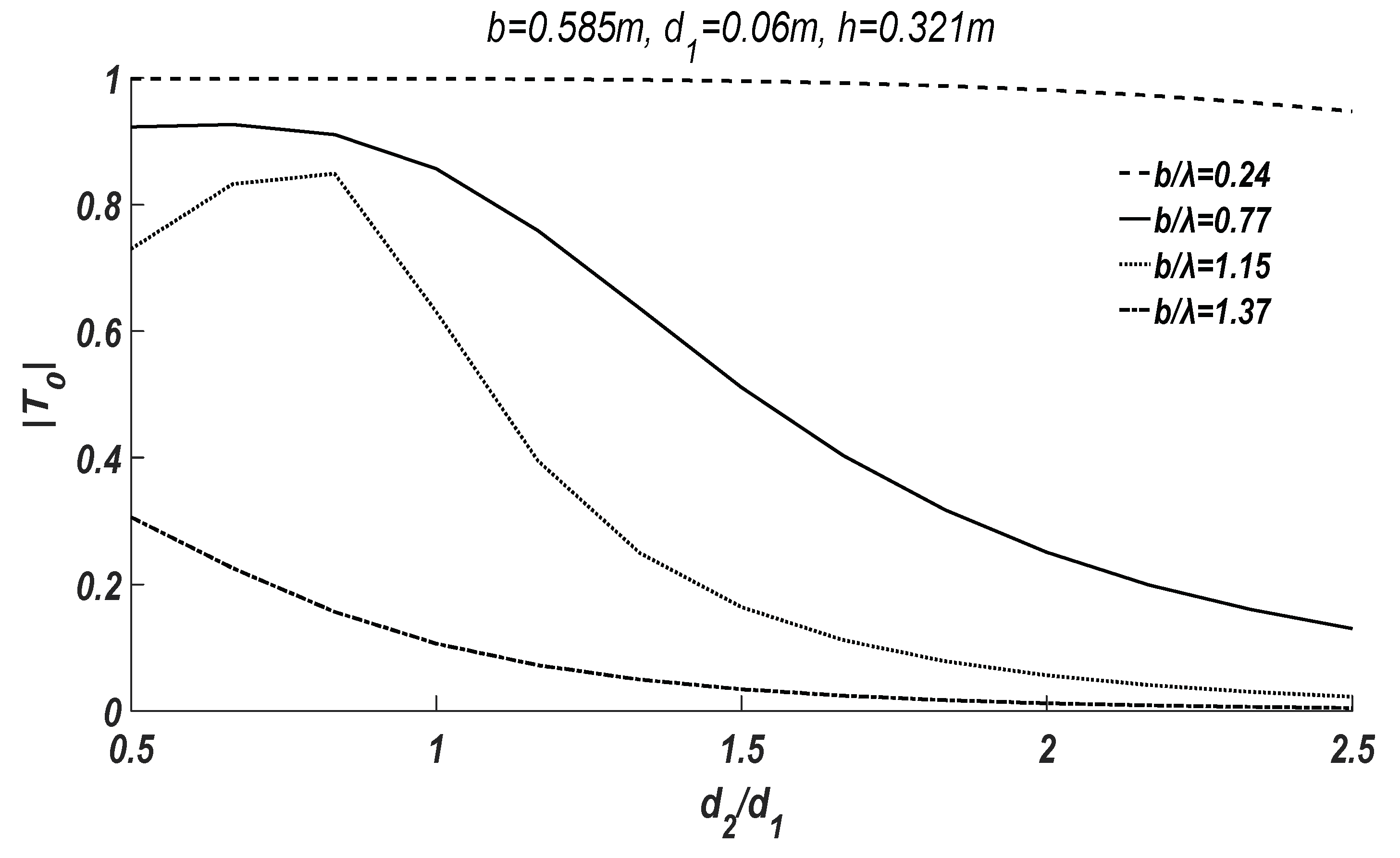
In this case, the draft of the first plate is fixed at , while the draft of the second one varies from to . Several groups of representative results with respect to different are shown in Figure 5.
Figure 5 clearly depicts the change of with respect to in different wavelengths. If the wavelength is much longer than the plate distance , e.g., , the increase of draft has little influence on the transmission coefficient. When the wavelength is comparable to the plate distance , e.g., , the increase of draft significantly reduces the transmission coefficient . In particular, in the vicinity of , the transmission coefficient firstly increases and then decreases with the growth of . On the other hand, when the wavelength is much smaller than the plate distance , e.g., , the transmission coefficient is dominant by the draft , which makes to be small even at , and with the growth of , the transmission coefficient gradually decreases to zero.
3.2. The Transmission of Progressive Waves Due to Multiple Plates
3.2.1. Effect of the Plate Number
The water depth is set as , and the distance between every two neighbouring plates is . The draft of all plates is set as . The number of plates is taken from 3 to 10. The transmission coefficients of progressive waves due to different number of plates are shown in Figure 6.
From Figure 6 one can find that, with the growth of the plate number, the progressive waves of long wavelength () almost propagate intact through the plates, i.e., in long waves the transmission coefficient is for an arbitrary plate number. On the other hand, in short to medium waves (), the transmission coefficient descends to zero with the growth of . However, in the vicinity of certain wavelengths () independent to the plate number, the transmission coefficient surges to a certain height and then follows back. Moreover, with the growth of the plate number, the surge tends to be multi-peak. These phenomena should associate with the standing waves between plates, which occur in certain conditions, and make the progressive waves pass through multiple plates with little reflection. Certainly, with the growth of the plate number, some wave energy is inevitably reflected and the surge amplitude of the transmission coefficient would decrease as compared to the two plate case.
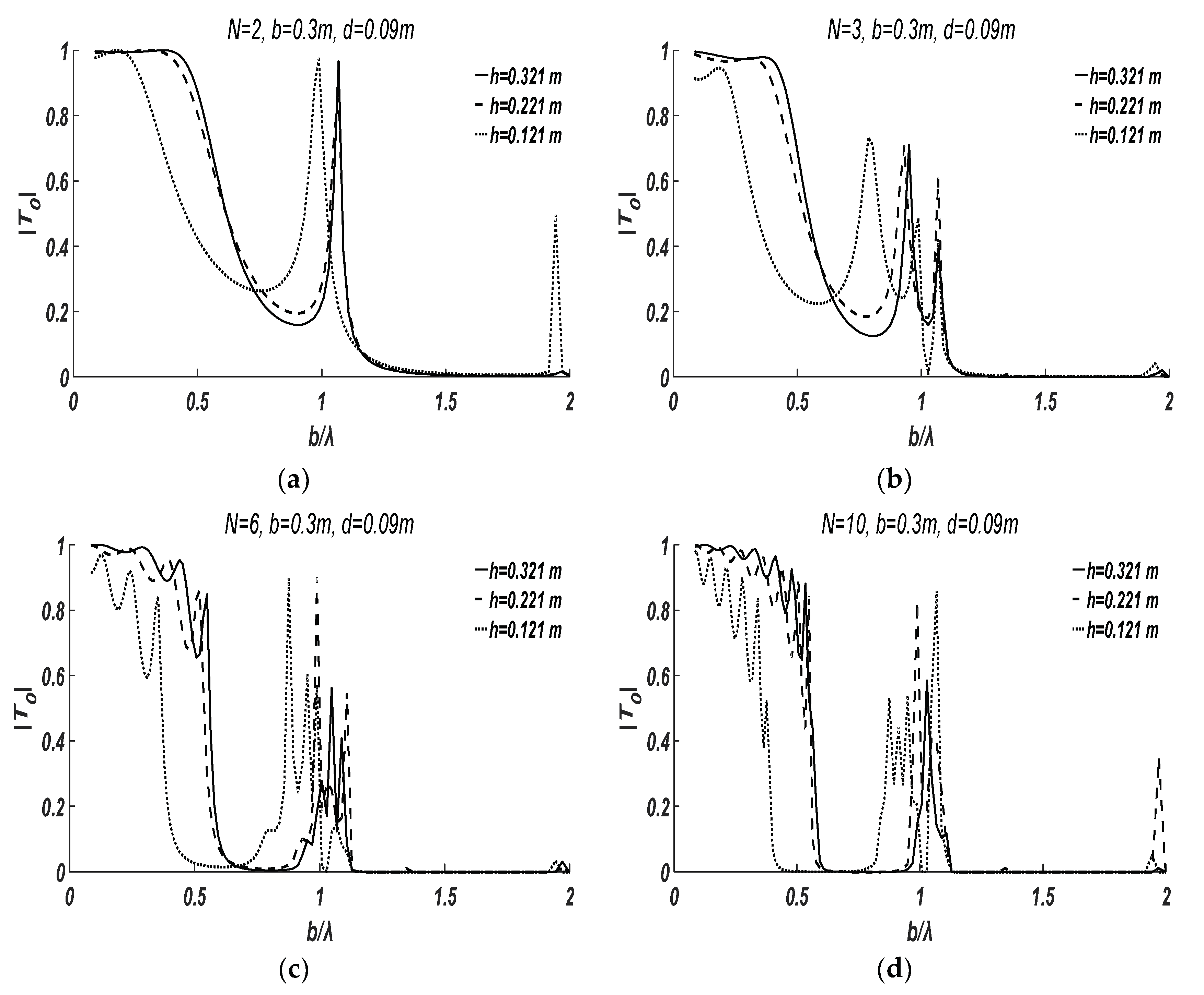
3.2.2. Effect of the Plate Draft to Water Depth Ratio
In this case, the effect of plate draft to water depth ratio on the transmission coefficient is investigated. The draft of the plates is set as and the distance between neighbouring plates is set as , which could make the transmission coefficient more sensitive to the wavelength, according to the study in Section 3.1. Three water depths , are employed for the study. The corresponding plate draft to water depth ratios are . Note that in shallow water or larger plate draft to water depth ratio (), along the water depth direction most water is shielded by plates.
Figure 7 compares the transmission coefficient in different water depth. One can observe that in shallower water or larger plate draft to the water depth ratio ( or ), the entire transmission coefficient curves move toward the left direction of , i.e., the transmission coefficient starts to decrease in longer waves, while with the growth of the water depth or the reduction of the plate draft to water depth ratio ( or ), the transmission coefficient does not make significant changes.
It can be concluded that the larger plate draft to the water depth ratio (i.e., the greater portion of water shielded by plates), the smaller the transmission coefficient one obtains, and in the longer waves the transmission coefficient surges, i.e., standing waves between plates occur in the longer waves.
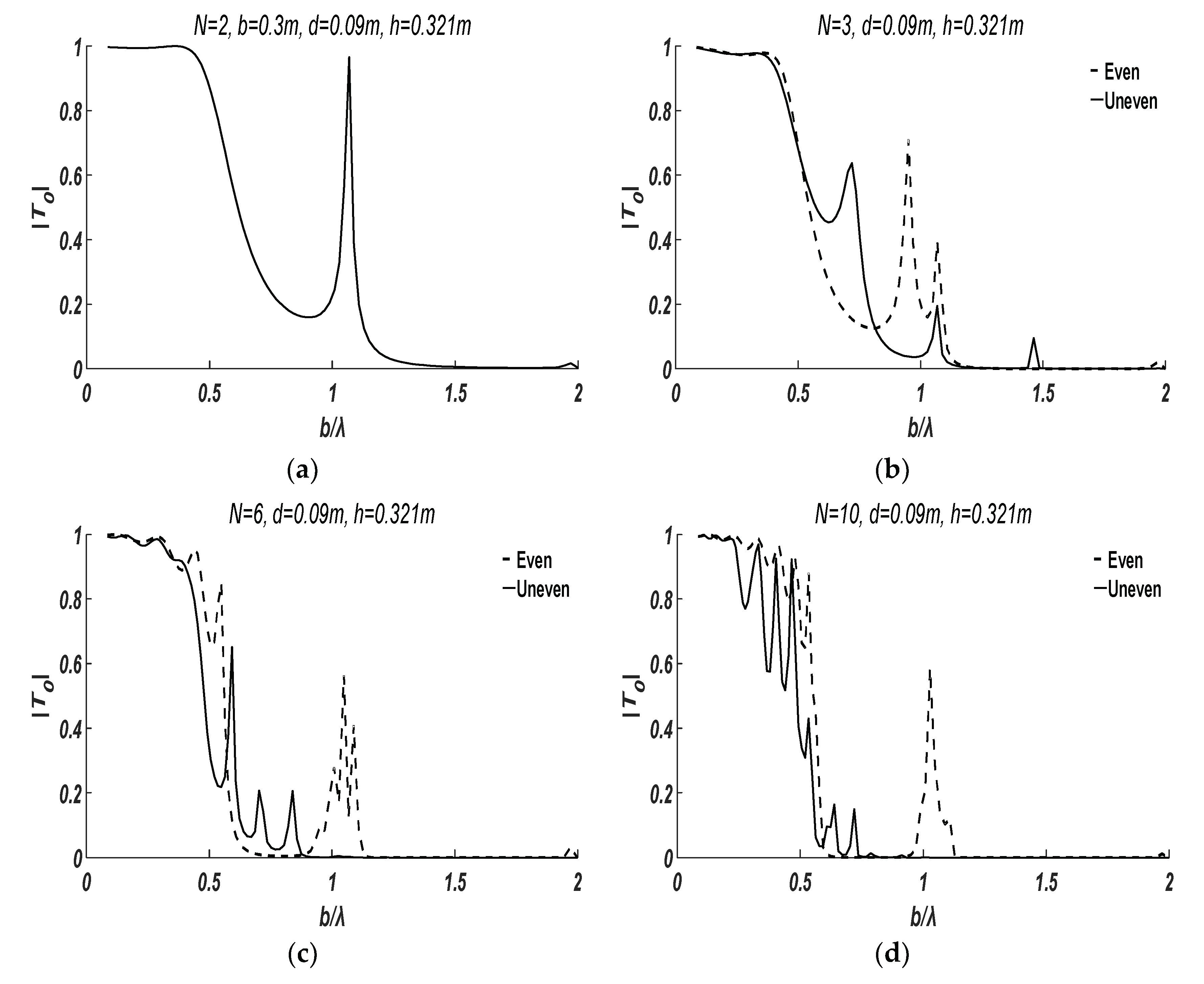
3.2.3. Effect of the Plate Arrangement
In this case, the influence of plate arrangement on the transmission coefficient is investigated. The draft of the plates is set as , and the depth of water is set as . For comparison purposes, two plate arrangements, even and uneven, are employed for the study. The distance between the first and th plate for these two arrangements can be written as:
Figure 8 portrays the transmission coefficient in the different plate arrangements. One can find that, in long waves (), the plate arrangement has little effect on the transmission coefficient, while, in medium waves (), the transmission coefficient due to uneven plate arrangement decreases more quickly with the increase of than the even case. Moreover, in short waves (), there are almost no significant transmission coefficient surges in the uneven plate arrangement case, as compared to the even plate arrangement case.
It is not surprising that the uneven plate arrangement can have such effects. As demonstrated in the Section 3.1.1, the occurrence of standing waves mainly relates to the plate distance to wavelength ratio . For the even arrangement plates with certain , the standing waves might appear between every pair of neighbouring plates and the progressive wave can pass through multiple plates and, finally, the transmission coefficient surges happen. For the uneven arrangement plates, however, the varies and it is difficult to produce standing waves between every pair of neighbouring plates, which results in the reflection of progressive wave, as well as the decrease of the transmission coefficient. The characteristic of an uneven arrangement of plates will benefit the design of floating breakwaters, which can more completely intercept the short waves than the conventional even plate arrangement.
4. Conclusions
In this paper, the analytical solution to the transmission of progressive water waves under multiple 2D vertical thin fixed plates is presented based on the linear potential theory, in which the number of plates can be arbitrary. The numerical model is validated through the case of two vertical thin plates, where the numerical results agree well with those from Shin and Cho [8].
The influences of relevant parameters, including the number of plates, the draft of plates, the distance between the plates, and the water depth on the transmission coefficient are investigated, which reflects the proportion of transmitted wave energy through the plates. The numerical results suggest that, with the growth of the plate draft or plate draft to water depth ratio, the transmission coefficient generally gradually decreases to zero, though some transmission coefficient surges that are associated with the standing waves between neighbouring plates appear in the certain waves; with the growth of plate number, the transmission coefficient surge tends to be multi-peak and the surge amplitude significantly decreases. Moreover, the plate arrangement has significant influence on the transmission coefficient. The uneven plate arrangement can suppress the production of standing waves between neighbouring plates and, thus, reduce the transmission coefficient.
It is worth noting that the analytical model and the numerical results proposed in this paper are within the linear and inviscid framework. The nonlinear and viscous effects of water waves are not taken into account. Nevertheless, the results of this paper contribute to the knowledge of the transmission of progressive water waves under multiple vertical thin plates, which can be employed for the optimal design of a floating breakwater with multiple plates.
Acknowledgments
This project is supported by the National Natural Science Foundation of China (grant no. 51579056, no. 51509053, and no. 51579051). The third author wishes to thank the Chang Jiang Visiting Chair professorship of Chinese Ministry of Education, supported and hosted by the Harbin Engineering University.
Author Contributions
Yifei Yu developed the mathematical model; Zhiqun Guo performed the numerical calculations; Qingwei Ma performed the analysis of the results; and Yifei Yu wrote the paper.
Conflicts of Interest
The authors declare no conflict of interest. The founding sponsors had no role in the design of the study; in the collection, analyses, or interpretation of data; in the writing of the manuscript; or in the decision to publish the results.
Appendix A
Using the separation variable method to solve the definite problem given in Equation (3). It is assumed that:
Substituting (A1) into Equation (3a), one obtains:
or:
where is independent of and . Thereby Equation (A3) can be transformed to:
In the following, three cases for solving the Equation (A4) are respectively discussed according to the value of :
(1)
Denoting , then from Equation (A4a) one can obtain:
Substituting Equation (A5) into (A1), and then into Equation (3b) and (3c) leads to:
where . The condition for the nonzero solution to Equation (A6) is:
The solution to Equation (A7) is , where:
Combining Equations (A5)–(A8), one obtains:
On the other hand, from Equation (A4b) one obtains:
Combining Equations (A9) and (A10), the velocity potential can be written as:
(2)
From Equation (A4a), it can be obtained that:
Substituting Equation (A12) into (A1), and then into Equation (3b) and (3c) yields:
Obviously, there only exist zero solutions to and , as well as to , and .
(3)
Denoting , then from Equation (A4a) one can obtain:
Substituting Equation (A12) into (A1), and then into Equation (3b) and (3c) comes to:
The condition for the nonzero solution to Equation (A15) is:
The solution to Equation (A16) is , where:
Combining Equations (A14)–(A17), one obtains:
On the other hand, from (A4b) one obtains:
Combining Equations (A18) and (A19) leads to the velocity potential:
References
- Wiegel, R.L. Transmission of waves past a rigid vertical thin barrier. J. Waterw. Harb. 1960, 86, 1–12. [Google Scholar]
- Kriebel, D.L.; Bollmann, C.A. Wave transmission past vertical wave barriers. Coast. Eng. Proc. 1996, 1, 2470–2483. [Google Scholar]
- Losada, I.J.; Losada, M.A.; Roldn, A.J. Propagation of oblique incident waves past rigid vertical thin barriers. Appl. Ocean Res. 1992, 14, 191–199. [Google Scholar] [CrossRef]
- Porter, R.; Evans, D.V. Complementary approximations to wave scattering by vertical barriers. J. Fluid Mech. 1995, 294, 155–180. [Google Scholar] [CrossRef]
- Srokosz, M.; Evans, D.V. A theory for wave-power absorption by two independently oscillating bodies. J. Fluid Mech. 1979, 90, 337–362. [Google Scholar] [CrossRef]
- Wu, J.; Liu, P.L. Interactions of obliquely incident water waves with two vertical obstacles. Appl. Ocean Res. 1988, 10, 66–73. [Google Scholar] [CrossRef]
- Liu, Y.; Li, Y.C. Wave interaction with a wave absorbing double curtain-wall breakwater. Ocean Eng. 2011, 38, 1237–1245. [Google Scholar] [CrossRef]
- Shin, D.M.; Cho, Y. Diffraction of waves past two vertical thin plates on the free surface: A comparison of theory and experiment. Ocean Eng. 2016, 124, 274–286. [Google Scholar] [CrossRef]
Figure 1.
The sketch of water waves under vertical thin plates. is the water depth, is the draft of th plate, is the distance from the th plate to the first plate, is the potential of progressive waves, is the potential of reflection wave, and is the potential of the transmission wave.
Figure 1.
The sketch of water waves under vertical thin plates. is the water depth, is the draft of th plate, is the distance from the th plate to the first plate, is the potential of progressive waves, is the potential of reflection wave, and is the potential of the transmission wave.

Figure 2.
Comparison of the transmission coefficient of progressive waves obtained using the present numerical model with the numerical results from Shin and Cho [8]. (a) The amplitude of the coefficient ; and (b) the phase of the coefficient .
Figure 2.
Comparison of the transmission coefficient of progressive waves obtained using the present numerical model with the numerical results from Shin and Cho [8]. (a) The amplitude of the coefficient ; and (b) the phase of the coefficient .

Figure 3.
The phase difference between the transmission coefficient on the first plate and the reflection coefficient on the second plate .
Figure 3.
The phase difference between the transmission coefficient on the first plate and the reflection coefficient on the second plate .

Figure 4.
Comparison of far-field transmission coefficient and near-field transmission coefficients with respect to plate distance to wavelength ratio .
Figure 4.
Comparison of far-field transmission coefficient and near-field transmission coefficients with respect to plate distance to wavelength ratio .

Figure 5.
The transmission coefficient of progressive waves with respect to different draft of the second plate . The draft of the first plate is fixed at .
Figure 5.
The transmission coefficient of progressive waves with respect to different draft of the second plate . The draft of the first plate is fixed at .

Figure 6.
The transmission coefficient of progressive waves under different number of plates. (a) Plate number . (b) Plate number . (c) Plate number . (d) Plate number .
Figure 6.
The transmission coefficient of progressive waves under different number of plates. (a) Plate number . (b) Plate number . (c) Plate number . (d) Plate number .

Figure 7.
The influence of plate draft to water depth ratio on the transmission coefficient of progressive waves. (a) Plate number . (b) Plate number . (c) Plate number . (d) Plate number .
Figure 7.
The influence of plate draft to water depth ratio on the transmission coefficient of progressive waves. (a) Plate number . (b) Plate number . (c) Plate number . (d) Plate number .

Figure 8.
The influence of plate arrangement on the transmission coefficient of progressive waves. (a) Plate number . (b) Plate number . (c) Plate number . (d) Plate number .
Figure 8.
The influence of plate arrangement on the transmission coefficient of progressive waves. (a) Plate number . (b) Plate number . (c) Plate number . (d) Plate number .

© 2018 by the authors. Licensee MDPI, Basel, Switzerland. This article is an open access article distributed under the terms and conditions of the Creative Commons Attribution (CC BY) license (http://creativecommons.org/licenses/by/4.0/).
Share and Cite
MDPI and ACS Style
Yu, Y.; Guo, Z.; Ma, Q. Transmission of Water Waves under Multiple Vertical Thin Plates. Water 2018, 10, 517. https://doi.org/10.3390/w10040517
AMA Style
Yu Y, Guo Z, Ma Q. Transmission of Water Waves under Multiple Vertical Thin Plates. Water. 2018; 10(4):517. https://doi.org/10.3390/w10040517
Chicago/Turabian StyleYu, Yifei, Zhiqun Guo, and Qingwei Ma. 2018. "Transmission of Water Waves under Multiple Vertical Thin Plates" Water 10, no. 4: 517. https://doi.org/10.3390/w10040517
Note that from the first issue of 2016, this journal uses article numbers instead of page numbers. See further details here.