Trends and Consumption Structures of China’s Blue and Grey Water Footprint

Abstract

Water footprint has become a common method to study the water resources utilization in recent years. By using input–output analysis and dilution theory, the internal water footprint, blue water footprint and grey water footprint of China from 2002 to 2012 were estimated, and the consumption structure of water footprint and virtual water trade were analyzed. The results show: (1) From 2002 to 2012, the average annual internal water footprint was 3.83 trillion m³ in China, of which the blue water footprint was 0.25 trillion m³, and the grey water footprint was 3.58 trillion m³ (with Grade III water standard accounting); both the internal water footprint and grey water footprint experienced decreasing trends from 2002 to 2012, except for a dramatic increase in 2010; (2) Average annual virtual blue water footprint was the greatest in agriculture (39.2%), while tertiary industry (27.5%) and food and tobacco processing (23.7%) were the top two highest for average annual virtual grey water footprint; (3) Virtual blue water footprint in most sectors showed increasing trends due to the increase of final demand, while virtual grey water footprint in most sectors showed decreasing trends due to the decreases of total return water coefficients and conversion coefficients of virtual grey water footprint; (4) For water resources, China was self-reliant: the water used for producing the products and services to meet domestic consumption was taken domestically; meanwhile, China exported virtual water to other countries, which aggravated the water stress in China.

1. Introduction

Water footprint refers to the water consumption for producing products and services for a certain population (individual, city or country) under certain material living standards [1]. This part of water resources includes not only the actual water used in daily life, water used for industrial and agricultural goods (services) production, and municipal water, but also the water used for processing sewage and waste water that is produced during the life and production activities. The concept of water footprint is actually a combination of physical and virtual water consumption, a combination of the consumption of “blue water” (surface water and groundwater) and “green water” (precipitation which does not form surface water, groundwater and is reserved in soil) [2], and a combination of changes in water quantity and quality. It shows the impact of human consumption on water resources from a broader view.

Raised by A. Y. Hoekstra in 2002, water footprint has been estimated at varies scales [3,4,5,6]. At a national level, Hoekstra and Chapagain carried out a systematic estimation of water footprint in 2007–2008 [7]. A. Y. Hoekstra et al. centralized years of research to compile the “Water Footprint Assessment Manual” [8], which was a comprehensive summary for water footprint analysis and could provide samples for water footprint research. Methods for calculating water footprint include bottom-up calculation method and top-down calculation method [1]. Input-output method, a top-down calculation method, has been widely used to study water footprint and virtual water [9,10,11,12,13]. For example, Zhao et al. used the input–output method to analyze the virtual water trade in China [12]; by combining an input–output model with intersectoral water flows, Wang et al. described a modified input–output model to calculate the gross water footprint of different sectors in Beijing [5]. By using the input–output method, the water consumption among sectors can be redistributed according to their input–output relations, thus obtaining the actual water consumption in each sector. However, though the input–output method has been widely applied to water footprint calculation, the grey water footprint calculation based on the input–output table has not been systematically studied.

Now researchers are trying to combine the bottom-up and top-down methods for better evaluating the water footprint. For example, Kang et al. applied a hybrid of bottom-up and top-down methods, from production and consumption perspectives, to calculate the water footprint for Xiamen city from 2001 to 2012 [14], which provided valuable information for a diverse set of water planning and water policy objectives [15]. Sun et al. quantitatively evaluated the water footprint, the intensity of water footprint and the external water dependency based on the top-down and bottom-up methods [16].

Additionally, in current macroscopic analysis, the water footprint self-reliance rate is often used, but mainly in areas where there is water footprint inflow, which could not reflect the status of areas where the water footprint outflow exists. Therefore, in this study, the water footprint macroscopic analysis indicators were improved based on virtual water trade. Virtual water trade indicates the embedded water trade accompanied with goods trade [17] and is a key procedure in reallocating the regional water resources, which provides a new way for solving the water scarcity in water-poor area [4,18]. Based on the assumption of balancing water resources through virtual water trade, many researchers made an estimation on virtual water trade [19,20], and some found that even water-poor regions still exported virtual water to other regions [3,13,21]. China is one of the 13 water-poor countries in the world and will face more serious water pressure with the rapid economic development and population expansion [18]. Therefore, the estimation of virtual water trade is necessary for gaining an insight into the water use pattern in China.

In this paper, the water footprint of different types and virtual water trade in China from 2002 to 2012 were calculated by using the input–output method and dilute theory. This paper aims to (1) estimate internal water footprint, blue water footprint and grey water footprint; (2) analyze the consumption structure of water footprint; and (3) discuss the virtual water trade in China.

2. Materials and Methods

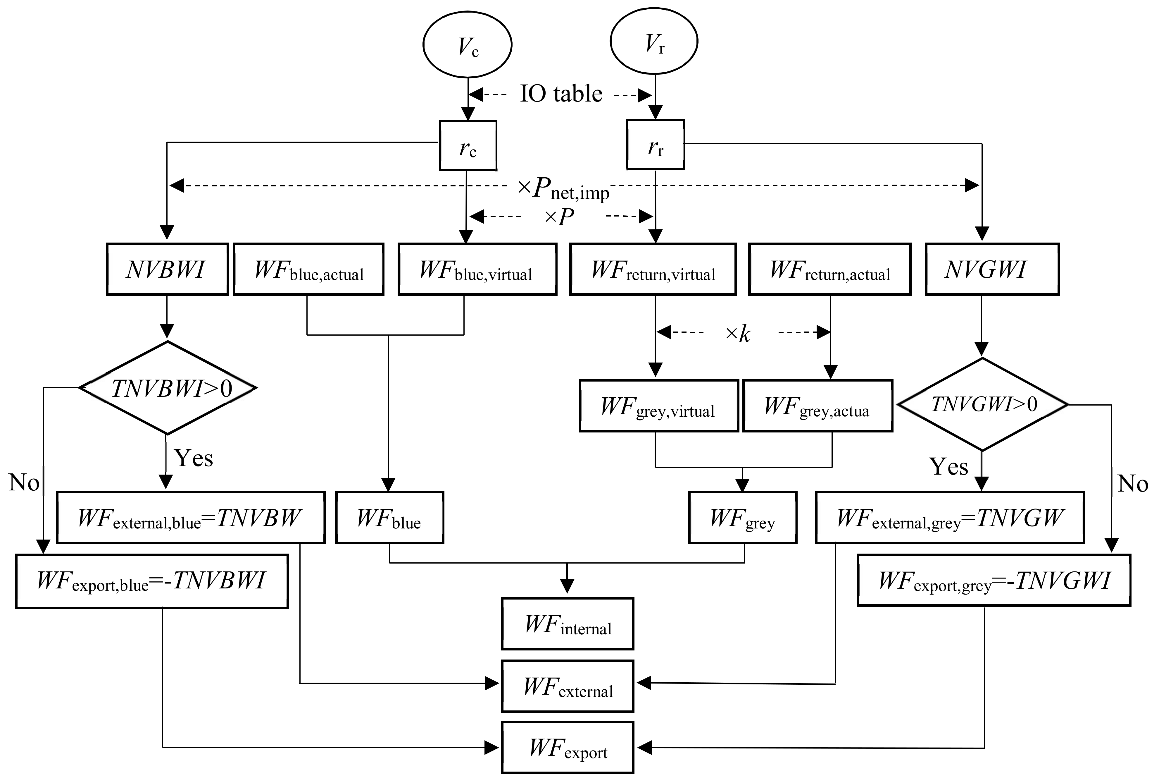
By using input–output analysis, the internal water footprint, blue water footprint and grey water footprint of China from 2002 to 2012 were estimated, and the consumption structure of water footprint and virtual water trade were analyzed. The calculation flow chart is shown in Figure 1.

2.1. Input–Output Table

In the input–output tables (IO table), the row model is shown as: ${\displaystyle \sum _{j=1}^{\mathrm{n}}{x}_{ij}+Y_i=X_i}$, where i indicates a certain sector in rows and j indicates a certain sector in columns; $x_{ij}$ is the input from sector i to sector j; $Y_i$ is the final demand in sector i; and $X_i$ is the total output in sector i.

$a_{ij}=x_{ij}/X_i$ is defined as the direct consumption coefficient, and $A={\left\{a_{ij}\right\}}_{n\times n}$ is the direct consumption coefficient matrix correspondingly; therefore, the row model can be expressed in matrix form as: $AX+Y=X$, where $X$ is the column vector of total output, $Y$ is the column vector of final demand. Therefore, we can get $X={(I-A)}^{-1}Y$, and then the complete demand matrix is defined as $B={(I-A)}^{-1}$, indicating the increase of output to meet one monetary unit increase of final use.

In this study, the input–output tables were aggregated into 26 sectors in order to match the water consumption and return water data. The 26 sectors are shown in

Table 1. Sectors of input–output table.

Sectors
1 Agriculture	14 Metal smelting and processing
2 Coal mining and processing	15 Metal products
3 Crude petroleum and natural gas extracting	16 General and specialized machinery
4 Metallic mining	17 Transport equipment
5 Non-metallic and other minerals mining	18 Electric equipment and machinery
6 Food and tobacco processing	19 Electronic and telecommunications equipment
7 Textile	20 Instruments, meters, cultural and office machinery
8 Garments, leather, furs, down	21 Scrap waste and other manufacturing products
9 Timber processing and furniture manufacturing	22 Electronic and heating power production and supply
10 Papermaking and cultural articles	23 Gas production and supply
11 Petroleum processing and coking	24 Water production and supply
12 Chemicals	25 Construction
13 Non-metal mineral products	26 Tertiary industry

.

2.2. Water Use, Water Consumption and Return Water

Water use refers to the amount of fresh water taken by water users. In the process of water transfer and water use, through evapotranspiration, soil absorption, product consumption, people and livestock drinking and other forms water consumption, some water cannot return to surface water or aquifer water, which is called water consumption. In the concept of water footprint, the amount of water should exclude the part of water returning to surface water and groundwater. Therefore, water consumption data should be used instead of water use data. The relationship among water use, water consumption and return water is as follows:

$$V_{\mathrm{u}}=[V_{\mathrm{u},j}],V_{\mathrm{c}}=[V_{\mathrm{c},j}],V_{\mathrm{r}}=[V_{\mathrm{r},j}],V_{\mathrm{u},j}=V_{\mathrm{c},j}+V_{\mathrm{r},j},$$

(1)

where $V_{\mathrm{u}}$ is the row vector of water use and $V_{\mathrm{u},j}$ is the water use in sector j (${\mathrm{m}}^3$); $V_{\mathrm{c}}$ is the row vector of water consumption and $V_{\mathrm{c},j}$ is the water consumption in sector j (${\mathrm{m}}^3$); $V_{\mathrm{r},j}$ is the row vector of return water and $V_{\mathrm{r},j}$ is the return water in sector j (${\mathrm{m}}^3$).

2.3. Water Consumption Coefficient and Return Water Coefficient

Referring to the concept of direct water use coefficient and total water use coefficient [6], we proposed direct water consumption coefficient, total water consumption coefficient, direct return water coefficient and total return water coefficient.

Direct water consumption coefficient refers to the water resources consumed in natural forms to increase one monetary unit output:

$$f_{\mathrm{c}}=[f_{\mathrm{c},j}],f_{\mathrm{c},j}=V_{\mathrm{c},j}/X_j,$$

(2)

where $f_{\mathrm{c}}$ is the row vector of direct water consumption coefficient and $f_{\mathrm{c},j}$ is the direct water consumption coefficient in sector j (${\mathrm{m}}^3/{10}^4\mathrm{Yuan}$); $X_j$ is the total output in sector j (${10}^4\mathrm{Yuan}$).

Direct return water coefficient refers to the amount of sewage and waste water discharged directly to produce one monetary unit output:

$$f_{\mathrm{r}}=[f_{\mathrm{r},j}],f_{\mathrm{r},j}=V_{\mathrm{r},j}/X_j,$$

(3)

where $f_{\mathrm{r},j}$ is the row vector of direct return water coefficient and $f_{\mathrm{r},j}$ is the direct return water coefficient in sector j (${\mathrm{m}}^3/{10}^4\mathrm{Yuan}$).

The total water consumption coefficient refers to the amount of water consumption in the whole production chain to increase one monetary output, consisting of direct water consumption coefficient ($f_{\mathrm{c}}$) and indirect water consumption coefficient ($f_{\mathrm{c},\mathrm{indirect}}$):

$$r_{\mathrm{c}}=f_{\mathrm{c}}\times B,$$

(4)

where $r_{\mathrm{c}}$ is the row vector of total water consumption coefficient (${\mathrm{m}}^3/{10}^4\mathrm{Yuan}$).

Similarly, the total return water coefficient refers to the amount of total return water in the whole production chain to increase one monetary unit output, consisting of direct return water coefficient ($f_{\mathrm{r}}$) and indirect return water consumption coefficient ($f_{\mathrm{r},\mathrm{indirect}}$):

$$r_{\mathrm{r}}=f_{\mathrm{r}}\times B,$$

(5)

where $r_{\mathrm{r}}$ is the row vector of total return water coefficient (${\mathrm{m}}^3/{10}^4\mathrm{Yuan}$).

2.4. Internal Water Footprint, Blue Water Footprint and Grey Water Footprint

Water footprint includes green water footprint, blue water footprint ($W{F}_{\mathrm{blue}}$) and grey water footprint ($W{F}_{\mathrm{grey}}$). Green water footprint and blue water footprint refer to the water consumption of green water and blue water during the production, respectively; grey water is the volume of water needed to dilute the pollutants [22,23]. Therefore, green water footprint and blue water footprint are related to the quantity of water resources, while grey water is related to the water quality.

This study focused on blue water footprint and grey water, but excluded green water footprint, because input–output analysis is sector-based, but green water footprint is always calculated based on the evapotranspiration of a specific crop; therefore, it is hard to determine which crops should be included in the calculation of agriculture (sector 1).

Internal water footprint ($W{F}_{\mathrm{internal}}$) denotes the domestic water needed for producing services and products consumed by domestic residents and consists of $W{F}_{\mathrm{blue}}$ and $W{F}_{\mathrm{grey}}$ in this study.

Blue water footprint consists of actual blue water footprint ($W{F}_{\mathrm{blue},\mathrm{actual}}$, $\mathrm{million}{\mathrm{m}}^3$) and virtual blue water footprint ($W{F}_{\mathrm{blue},\mathrm{virtual}}$, $\mathrm{million}{\mathrm{m}}^3$), where $W{F}_{\mathrm{blue},\mathrm{actual}}$ refers to the living water consumption, while $W{F}_{\mathrm{blue},\mathrm{virtual}}$ refers to the water used for producing the goods and services for consumption:

$$W{F}_{\mathrm{blue},\mathrm{virtual}}=[W{F}_{\mathrm{blue},\mathrm{virtual},j}],P=[P_j],W{F}_{\mathrm{blue},\mathrm{virtual},j}=r_{\mathrm{c},j}\times P_j/{10}^6,$$

(6)

where $W{F}_{\mathrm{blue},\mathrm{virtual}}$ is the row vector of virtual blue water footprint and $W{F}_{\mathrm{blue},\mathrm{virtual},j}$ is the virtual blue water footprint in sector j; $P$ is the row vector of expenditure and $P_j$ is the expenditure in sector j (${10}^4\mathrm{Yuan}$).

Similar with the blue water footprint, return water also includes actual return water ($W{F}_{\mathrm{return},\mathrm{actual}}$, $\mathrm{million}{\mathrm{m}}^3$) and virtual return water ($W{F}_{\mathrm{return},\mathrm{virtual}}$, $\mathrm{million}{\mathrm{m}}^3$), which are caused by living return water and the return water generated in producing the goods and services for domestic consumption, respectively:

$$W{F}_{\mathrm{return},\mathrm{virtual}}=[W{F}_{\mathrm{return},\mathrm{virtual},j}],W{F}_{\mathrm{return},\mathrm{virtual},j}=r_{\mathrm{r},j}\times P_j/{10}^6,$$

(7)

where $W{F}_{\mathrm{return},\mathrm{virtual}}$ is the row vector of virtual return water footprint and $W{F}_{\mathrm{return},\mathrm{virtual}}$ is the virtual return water footprint in sector j.

In calculating the grey water footprint, we need to consider both the volume and pollutant concentration of the waste water, and the water quality standard and the concentration of background pollutants. Since different pollutants can be diluted in the meantime, the pollutants chosen for calculation should be those that can cause the maximum grey water footprint. In this study, two biggest pollutants, COD (Chemical Oxygen Demand) and NH₃-N (Ammonia Nitrogen), were chosen as the particular pollutants to analyze the grey water footprint.

Define $k$ as the row vector of conversion coefficient of grey water footprint, where $k_j$ for second and tertiary industrial sector j and $k_{\mathrm{actual}}$ for living return water. The grey water footprint can be calculated as:

$$k=[k_j,k_{\mathrm{actual}}],k_j(k_{\mathrm{actual}})=\max \left\{\frac{c_{\mathrm{COD},j}(c_{\mathrm{COD},\mathrm{actual}})}{c_{\max ,\mathrm{COD}}-c_{\mathrm{nat}}},\frac{c_{{\mathrm{NH}}_3-\mathrm{N},j}(c_{{\mathrm{NH}}_3-\mathrm{N},\mathrm{actual}})}{c_{\max ,{\mathrm{NH}}_3-\mathrm{N}}-c_{\mathrm{nat}}}\right\},$$

(8)

$$W{F}_{\mathrm{grey},\mathrm{virtual}}=[W{F}_{\mathrm{grey},\mathrm{virtual},j}],W{F}_{\mathrm{grey},\mathrm{virtual},j}=k_j\times W{F}_{\mathrm{return},\mathrm{virtual},j},$$

(9)

$$W{F}_{\mathrm{grey},\mathrm{actual}}=k_{\mathrm{actual}}\times W{F}_{\mathrm{return},\mathrm{actual}},$$

(10)

where $W{F}_{\mathrm{grey},\mathrm{virtual}}$ is the row vector of virtual grey water footprint and $W{F}_{\mathrm{grey},\mathrm{virtual},j}$ refers to the virtual grey water footprint in sector j ($\mathrm{million}{\mathrm{m}}^3$); $W{F}_{\mathrm{grey},\mathrm{actual}}$ is the grey water footprint of domestic living, ($\mathrm{million}{\mathrm{m}}^3$); $c_{\mathrm{COD},j}$ and $c_{{\mathrm{NH}}_3-\mathrm{N},j}$ refer to the COD and NH₃-N concentrations in sector j, respectively ($\mathrm{mg}/\mathrm{L}$); $c_{\max ,\mathrm{COD}}$ and $c_{\max ,{\mathrm{NH}}_3-\mathrm{N}}$ are the maximum allowable pollutants concentrations ($\mathrm{mg}/\mathrm{L}$) for COD and NH₃-N of Grade III water, which are 20 mg/L and 1 mg/L, respectively, according to the China Environmental Quality Standard for Surface Water (GB3838-2002); $c_{\mathrm{nat}}$ is the concentration of background pollutants in natural condition ($\mathrm{mg}/\mathrm{L}$), and is assumed to be zero as the concentration is very low under natural condition.

For agriculture, the grey water footprint was calculated as:

$$W{F}_{\mathrm{grey},\mathrm{agri}}=\frac{\alpha \times \mathrm{Appl}}{c_{\max }-c_{\mathrm{nat}}}\times {10}^4,$$

(11)

where $\alpha$ denotes the nitrogen leaching loss rate, which is 7% on average in China [24]; $\mathrm{Appl}$ denotes the quantity of nitrogen fertilizer (${10}^4\mathrm{ton}$); $c_{\max }$ are the maximum allowable pollutants concentration ($\mathrm{mg}/\mathrm{L}$) for nitrate, which is 10 mg/L according to the China Environmental Quality Standard for Surface Water (GB3838-2002).

2.5. External Water Footprint and Water Footprint Export

When there is goods and services trade among countries, there is virtual blue water and virtual return water trade. The net virtual blue water import ($NVBWI$, $\mathrm{million}{\mathrm{m}}^3$) and net virtual grey water import ($NVGWI$, $\mathrm{million}{\mathrm{m}}^3$) can indicate the underlying blue water and grey water transfer with trade activity, respectively. This study assumes imported goods had the same total water consumption coefficient and total return water coefficient with the domestic one:

$$NVBWI=[NVBW{I}_j],NVBW{I}_j=r_{\mathrm{c},j}\times P_{\mathrm{net},\mathrm{imp},j}/{10}^6,$$

(12)

$$NVGWI=[NVGW{I}_j],NVGW{I}_j=k_j\times r_{\mathrm{r},j}\times P_{\mathrm{net},\mathrm{imp},j}/{10}^6,$$

(13)

where $NVBWI$ is the row vector of net virtual blue water import and $NVBW{I}_j$ refers to the net virtual blue water import in sector j; $NVGWI$ is the row vector of net virtual grey water import and $NVGW{I}_j$ refers to the net virtual grey water import in sector j; $P_{\mathrm{net},\mathrm{imp},j}$ (${10}^4\mathrm{Yuan}$) is the net import of sector j.

The positive $NVBWI$ and $NVGWI$ indicate a net virtual blue/grey water import, implying a water stress alleviation of China by importing virtual water through trade activities; while the negative $NVBWI$ and $NVGWI$ indicate a net virtual blue/grey water export, implying that the water stress in China is aggravated by exporting virtual water to other countries through trade activities.

If the total net virtual water import ($TNVBWI$) or total net virtual return water import ($TNVGWI$) is positive, it is defined as the external water footprint ($W{F}_{\mathrm{external}}$, $\mathrm{million}{\mathrm{m}}^3$), indicating the total net virtual water import for domestic consumption. It consists of external blue water footprint ($W{F}_{\mathrm{external},\mathrm{blue}}$, $\mathrm{million}{\mathrm{m}}^3$) and external grey water footprint ($W{F}_{\mathrm{external},\mathrm{grey}}$, $\mathrm{million}{\mathrm{m}}^3$) [25].

$$TNVBWI={\displaystyle \sum NVBW{I}_j},$$

(14)

$$TNVGWI={\displaystyle \sum NVGW{I}_j},$$

(15)

$$W{F}_{\mathrm{external},\mathrm{blue}}=\max \left\{TNVBWI,0\right\},$$

(16)

$$W{F}_{\mathrm{external},\mathrm{grey}}=\max \left\{TNVGWI,0\right\}.$$

(17)

When $TNVBWI$ or $TNVGWI$ is negative, its opposite number is defined as the water footprint export ($W{F}_{\mathrm{export}}$, $\mathrm{million}{\mathrm{m}}^3$), indicating the total net virtual water export for abroad consumption. It consists of blue water footprint export ($W{F}_{\mathrm{export},\mathrm{blue}}$, $\mathrm{million}{\mathrm{m}}^3$) and grey water footprint export ($W{F}_{\mathrm{export},\mathrm{grey}}$, $\mathrm{million}{\mathrm{m}}^3$):

$$W{F}_{\mathrm{export},\mathrm{blue}}=\max \left\{-TNVBWI,0\right\},$$

(18)

$$W{F}_{\mathrm{export},\mathrm{grey}}=\max \left\{-TNVGWI,0\right\}.$$

(19)

Based on the conceptions of external water footprint and water footprint export, two indices, water self-reliance (WSR) and water export fraction (WEF), were proposed. The level of WSR denotes how much the local consumption relies on local water resources. WSR is one hundred percent if a country was a net virtual water export country; it approaches zero if a country heavily relied on virtual water import.

$$WSR=\frac{W{F}_{\mathrm{internal}}}{W{F}_{\mathrm{internal}}+W{F}_{\mathrm{external}}}\times 100\%.$$

(20)

WEF reflects how much a country exports virtual water abroad. If WEF is zero, the country exports no virtual water abroad, i.e., the country is a net virtual water import country. The larger WEF is, the more the country exports virtual water to other countries.

$$WEF=\frac{W{F}_{\mathrm{export}}}{W{F}_{\mathrm{internal}}+W{F}_{\mathrm{export}}}\times 100\%.$$

(21)

2.6. Materials

Data used in this study includes the 42-sector input–output tables of China in 2002, 2005, 2007, 2010 and 2012, water consumption, return flow, NH₃-N and COD contents in the corresponding sectors, and the annual quantity of nitrogen fertilizer in China.

Therein, the input–output tables of China were obtained from Chinese Input–Output Association (http://www.stats.gov.cn/ztjc/tjzdgg/trccxh/). Agricultural water consumption is the product of agricultural water use and agricultural water consumption rate obtained from China Water Resources Bulletin. For the second industry, water consumption is the difference of water use and return water obtained from the China Environment Yearbook and China Statistical Yearbook on Environment in 2002 and 2005; especially, water use in 2007, 2010 and 2012 were calculated using return water and the corresponding water consumption rates which were estimated as the average value of those in the last two years. Living water consumption and tertiary industrial water consumption were identified by living water, public water and the corresponding water consumption rates obtained from the China Water Resources Bulletin. On the balance of the total volume, water consumption and return flow in each industrial sector was adjusted in equal proportion to meet the total volume provided by China Water Resources Bulletin. It should be noted that the return water in the China Water Resources Bulletin does not include the discharge of thermal power dc cooling water and mine return water, which can make the grey water footprint in this study a bit underestimated. NH₃-N and COD concentrations in sectors were determined according to the statistical data in China Environment Yearbook and China Statistical Yearbook on Environment. In particular, the NH₃-N and COD concentrations in tertiary industry referred to that in living return water for substitution. Quantity of nitrogen fertilizer was obtained from China Statistical Yearbook. All input data are available in Supplementary Materials.

3. Results

3.1. Internal Water Footprint

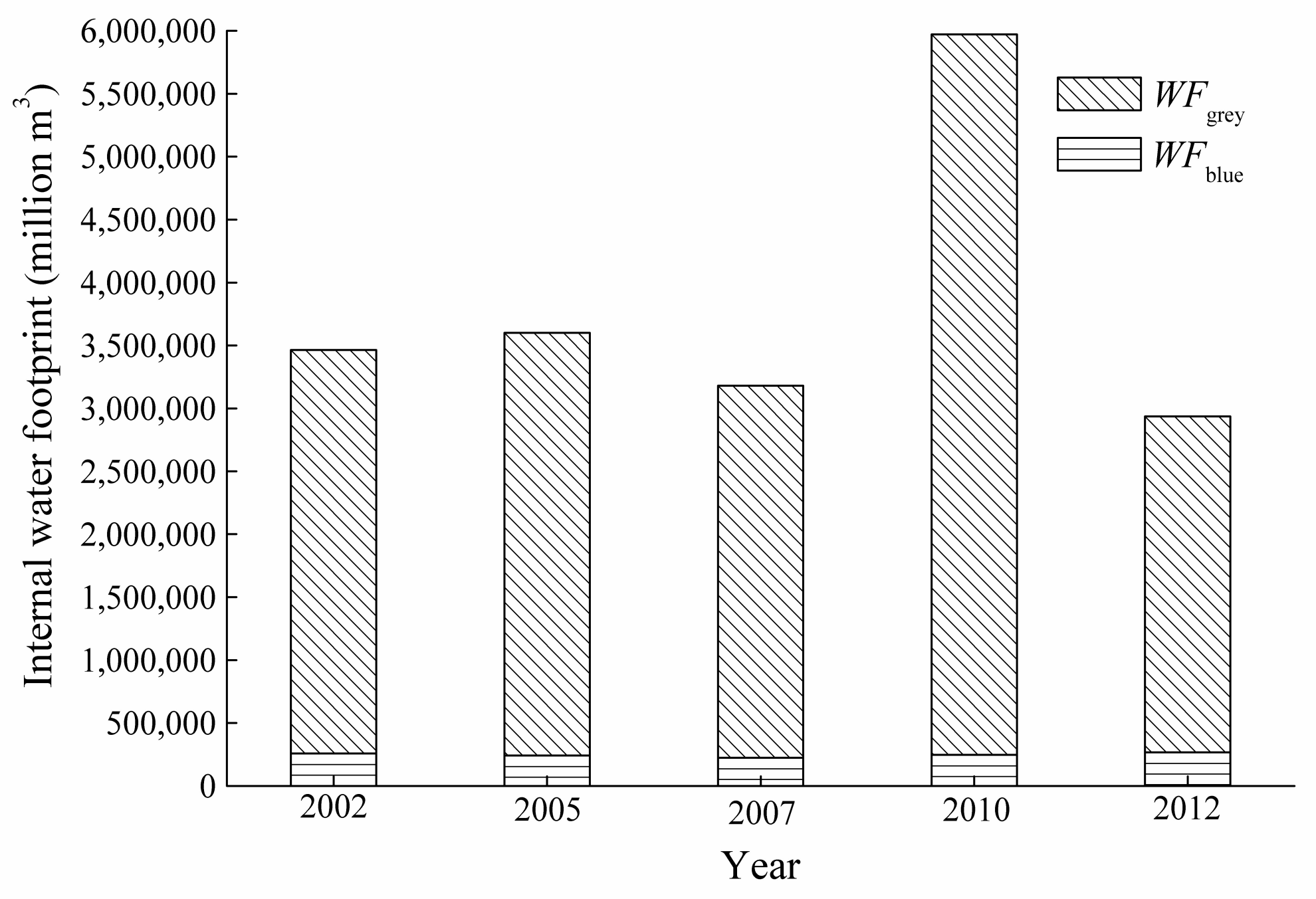
From 2002 to 2012, the average annual internal water footprint was 3.83 trillion m³ in China, of which the blue water footprint was 0.25 trillion m³ and the grey water footprint was 3.58 trillion m³ (with Grade III water standard accounting). Grey water footprint greatly dominated the internal water footprint and accounted for 93% on average of the internal water footprint, ranging from 91% to 96% during the study period. The internal water footprint overall showed a decreasing trend from 2002 to 2012, except for a dramatic increase in 2010 due to the increase of grey water footprint, blue water footprint did not change significantly, while grey water footprint showed consistent trend with internal water footprint. It is because since 2008, volume of return water in sector 25 experienced a dominant decreasing trend; however, COD and NH₃-N emissions kept a relatively stable level according to the China Statistical Yearbook on Environment, which resulted in a larger conversion coefficient that caused a dramatic increase of grey water footprint in 2010. Changes of internal water footprint and its compositions are shown in Figure 2.

3.2. The Consumption Structure of Blue Water Footprint

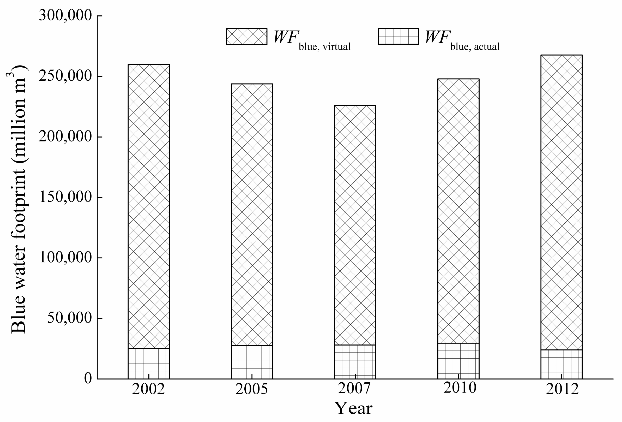
From 2002 to 2012, the annual average of $W{F}_{\mathrm{blue},\mathrm{actual}}$ was 0.03 trillion m³, and the annual average of $W{F}_{\mathrm{blue},\mathrm{virtual}}$ was 0.22 trillion m³; virtual blue water footprint occupied a large proportion (89%) of the blue water footprint, while the proportion of actual water consumption was almost negligible, indicating that the consumption of goods and services for final use was the major way to produce blue water footprint. Figure 3 shows the inter-annual variations of $W{F}_{\mathrm{blue}}$ and its compositions from 2002 to 2012, it is obvious that $W{F}_{\mathrm{blue},\mathrm{virtual}}$ first decreased from 2002 to 2005, and then increased continuously and slightly from 2005 to 2012. $W{F}_{\mathrm{blue},\mathrm{actual}}$ was relatively stable.

Table 2. Sectoral virtual blue water footprint of China from 2002 to 2012. (unit: million m³).

Sectors	2002	2005	2007	2010	2012	Average	Proportions	Trend
1	119,418	85,386	73,824	64,867	91,529	87,005	39.2%	−2.2%
2	192	−556	52	66	62	−37	0.0%	−14.7%
3	13	4	10	14	17	12	0.0%	4.4%
4	12	303	29	98	7	90	0.0%	−4.9%
5	10	−57	1	12	−11	−9	0.0%	−7.9%
6	29,952	39,580	45,420	57,786	60,435	46,635	21.0%	4.6%
7	1742	1063	869	812	1164	1130	0.5%	−3.1%
8	3584	5612	6232	7557	6952	5988	2.7%	3.8%
9	916	515	2044	1822	1938	1447	0.7%	6.3%
10	434	421	336	588	1177	591	0.3%	9.3%
11	49	341	194	286	493	273	0.1%	9.6%
12	1740	283	1661	2188	2690	1712	0.8%	6.5%
13	236	311	110	198	83	188	0.1%	−4.9%
14	11	−2	252	298	38	119	0.1%	6.3%
15	401	−48	513	305	664	367	0.2%	7.5%
16	2638	4404	3957	5241	5021	4252	1.9%	3.5%
17	1539	2383	3384	5805	5280	3678	1.7%	8.3%
18	708	1303	1942	3216	2153	1865	0.8%	6.7%
19	1091	1110	1053	1527	1048	1166	0.5%	0.7%
20	80	244	187	244	129	177	0.1%	1.3%
21	740	1,134	1259	1923	67	1025	0.5%	−1.1%
22	2640	1523	2,237	1860	1312	1915	0.9%	−2.8%
23	133	156	76	163	130	131	0.1%	0.0%
24	106	90	119	289	133	148	0.1%	4.2%
25	36,210	38,609	19,734	23,791	25,287	28,726	12.9%	−3.1%
26	29,822	32,140	32,377	37,430	35,878	33,529	15.1%	1.3%

shows the sectoral $W{F}_{\mathrm{blue},\mathrm{virtual}}$ of China from 2002 to 2012. Virtual blue water footprint in agriculture (sector 1) was the largest, with an average value of 87 billion m³, accounting for 39.2% of the total virtual blue water footprint, followed by that in sector 6 (food and tobacco processing) which was 46.6 billion m³, accounting for 21% of the total virtual blue water footprint. Nineteen out of twenty-four industrial sectors had the proportions of $W{F}_{\mathrm{blue},\mathrm{virtual}}$ over total virtual blue water footprint less than one percent. $W{F}_{\mathrm{blue},\mathrm{virtual}}$ of tertiary industry (sector 26) was 33.5 billion m³, accounting for 15.1% of the total virtual blue water footprint. Change trends of $W{F}_{\mathrm{blue},\mathrm{virtual}}$ varied among different sectors. Seventeen out of twenty-six sectors had $W{F}_{\mathrm{blue},\mathrm{virtual}}$ increased, among which $W{F}_{\mathrm{blue},\mathrm{virtual}}$ in sector 11 (petroleum processing and coking) increased the fastest during the study period, with an average increase rate of 9.6%; followed by that in sector 10 (papermaking and cultural articles) and sector 17 (transport equipment), of which the increase rates were 9.3% and 8.3%, respectively. $W{F}_{\mathrm{blue},\mathrm{virtual}}$ in sector 2 (coal mining and processing) decreased the fastest, with an average decrease rate of −14.7%, followed by that in sector 5 (non-metallic and other minerals mining) whose decrease rate was −7.9%. $W{F}_{\mathrm{blue},\mathrm{virtual}}$ in sector 19 (electronic and telecommunications equipment) and sector 23 (gas production and supply) had very small changes, with the change rates less than one percent.

Virtual blue water footprint was caused by rural residents’ consumption (23%), urban residents’ consumption (42%), government consumption (7%), gross fixed capital formation and inventory investment (28%).

For the $W{F}_{\mathrm{blue},\mathrm{virtual}}$ caused by rural residents’ consumption (

Table 3. Average volumes and change trends of $W{F}_{\mathrm{blue},\mathrm{virtual}}$ and $W{F}_{\mathrm{grey},\mathrm{virtual}}$ caused by rural residents’ consumption, urban residents’ consumption and government consumption from 2002 to 2012. (unit: million m³).

Sectors	Virtual Blue Water Footprint						Virtual Grey Water Footprint
	Rural		Urban		Government		Rural		Urban		Government
	Volume	Trend	Volume	Trend	Volume	Trend	Volume	Trend	Volume	Trend	Volume	Trend
1	32,280	−4.4%	38,451	−2.8%	1880	0.9%	22,025	−3.9%	26,225	−2.3%	1299	1.2%
2	23	−5.4%	33	−11.1%	0	-	158	−6.1%	227	−12.0%	0	-
3	0	-	2	−20.0%	0	-	0	-	30	−20.0%	0	-
4	0	-	0	-	0	-	0	-	0	-	0	-
5	1	−15.8%	3	−15.9%	0	-	9	−15.7%	32	−15.8%	0	-
6	12,444	3.8%	30,278	6.1%	0	-	181,698	−3.2%	416,796	−1.0%	0	-
7	385	−4.5%	743	−6.6%	0	-	2660	−6.0%	5222	−7.9%	0	-
8	980	6.1%	4628	4.1%	0	-	16,725	0.8%	82,455	−1.1%	0	-
9	136	1.7%	534	0.9%	0	-	1857	−6.2%	7361	−6.6%	0	-
10	73	9.0%	371	6.7%	0	-	1816	−4.5%	9572	−3.9%	0	-
11	27	2.8%	185	16.1%	0	-	352	−4.5%	1827	9.9%	0	-
12	430	−0.8%	1242	6.5%	0	-	13,510	−7.1%	34,077	−2.3%	0	-
13	31	−7.4%	139	−8.4%	0	-	176	−9.7%	812	−10.0%	0	-
14	2	−16.0%	4	−15.9%	0	-	20	−15.4%	43	−15.4%	0	-
15	28	−5.0%	122	−3.9%	0	-	120	−2.9%	527	−1.7%	0	-
16	4	8.9%	25	0.4%	0	-	33	−7.2%	241	−8.0%	0	-
17	133	1.9%	537	12.2%	0	-	911	1.5%	3648	10.2%	0	-
18	127	3.8%	468	1.8%	0	-	611	3.7%	2256	2.0%	0	-
19	65	3.8%	271	1.4%	0	-	367	4.6%	1503	2.6%	0	-
20	6	1.0%	18	2.6%	0	-	32	0.7%	110	2.6%	0	-
21	108	−1.6%	539	−2.3%	0	-	770	−6.2%	3823	−6.4%	0	-
22	378	−1.3%	1537	−3.2%	0	-	344	0.0%	1417	−1.9%	0	-
23	7	10.7%	121	−0.6%	0	-	358	5.2%	7603	−5.5%	0	-
24	16	0.8%	132	4.6%	0	-	107	−1.5%	941	1.8%	0	-
25	0	-	122	5.0%	0	-	0	-	10,226	8.4%	0	-
26	3701	−1.0%	13,373	1.7%	13,054	0.6%	88,061	−2.5%	312,846	0.3%	307,480	−0.9%

- denotes that there is no data for this cell because the volume in each year was zero.

), agriculture (sector 1) contributed the most, of which the $W{F}_{\mathrm{blue},\mathrm{virtual}}$ on average was as high as 32.3 billion m³, accounting for 62.8% of the total $W{F}_{\mathrm{blue},\mathrm{virtual}}$ caused by rural residents’ consumption, followed by sector 6 (food and tobacco processing), of which the $W{F}_{\mathrm{blue},\mathrm{virtual}}$ on average was 12.4 billion m³, accounting for 24.2%. Thirteen out of twenty-six sectors had very small $W{F}_{\mathrm{blue},\mathrm{virtual}}$ caused by rural residents’ consumption, all accounting for less than 0.1%. As for change trends, $W{F}_{\mathrm{blue},\mathrm{virtual}}$ caused by rural residents’ consumption in sector 14 (metal smelting and processing) and sector 5 (non-metallic and other minerals mining) presented the greatest and second greatest decreasing trends, with the decrease rates of −16% and −15.8%, respectively; while $W{F}_{\mathrm{blue},\mathrm{virtual}}$ caused by rural residents’ consumption in sector 23 (electronic and heating power production and supply) and sector 10 (papermaking and cultural articles) presented the greatest and second greatest increasing trends, with the increase rates of 10.7% and 9%, respectively.

Among the $W{F}_{\mathrm{blue},\mathrm{virtual}}$ caused by urban residents’ consumption, agriculture (sector 1) also contributed the most, of which the $W{F}_{\mathrm{blue},\mathrm{virtual}}$ on average was 38.5 billion m³, accounting for 41% of the total $W{F}_{\mathrm{blue},\mathrm{virtual}}$ caused by urban residents’ consumption, followed by sector 6, of which the $W{F}_{\mathrm{blue},\mathrm{virtual}}$ on average was 30.3 billion m³, accounting for 32.3%. Seven out of twenty-six sectors had very small $W{F}_{\mathrm{blue},\mathrm{virtual}}$ caused by urban residents’ consumption, all accounting for less than 0.1%. As for change trends, eleven out of twenty-six sectors showed decreasing trends. $W{F}_{\mathrm{blue},\mathrm{virtual}}$ caused by urban residents’ consumption in sector 3 (crude mining and processing), sector 5 (non-metallic and other minerals mining) and sector 14 (metal smelting and processing) showed the top three greatest decreasing trends, with the decrease rates of −20%, −15.9% and −15.9%, respectively; while $W{F}_{\mathrm{blue},\mathrm{virtual}}$ caused by urban residents’ consumption in sector 11 (petroleum processing and coking) and sector 17 (transport equipment) showed the greatest and second greatest increasing trends, with the increase rates of 16.1% and 12.2%, respectively.

For $W{F}_{\mathrm{blue},\mathrm{virtual}}$ caused by government consumption, it concentrated in tertiary industry (sector 26) and agriculture (sector 1), which were 13.1 billion m³ and 18.8 billion m³, accounting for 87.4% and 12.6% of the total $W{F}_{\mathrm{blue},\mathrm{virtual}}$ caused by government consumption, respectively.

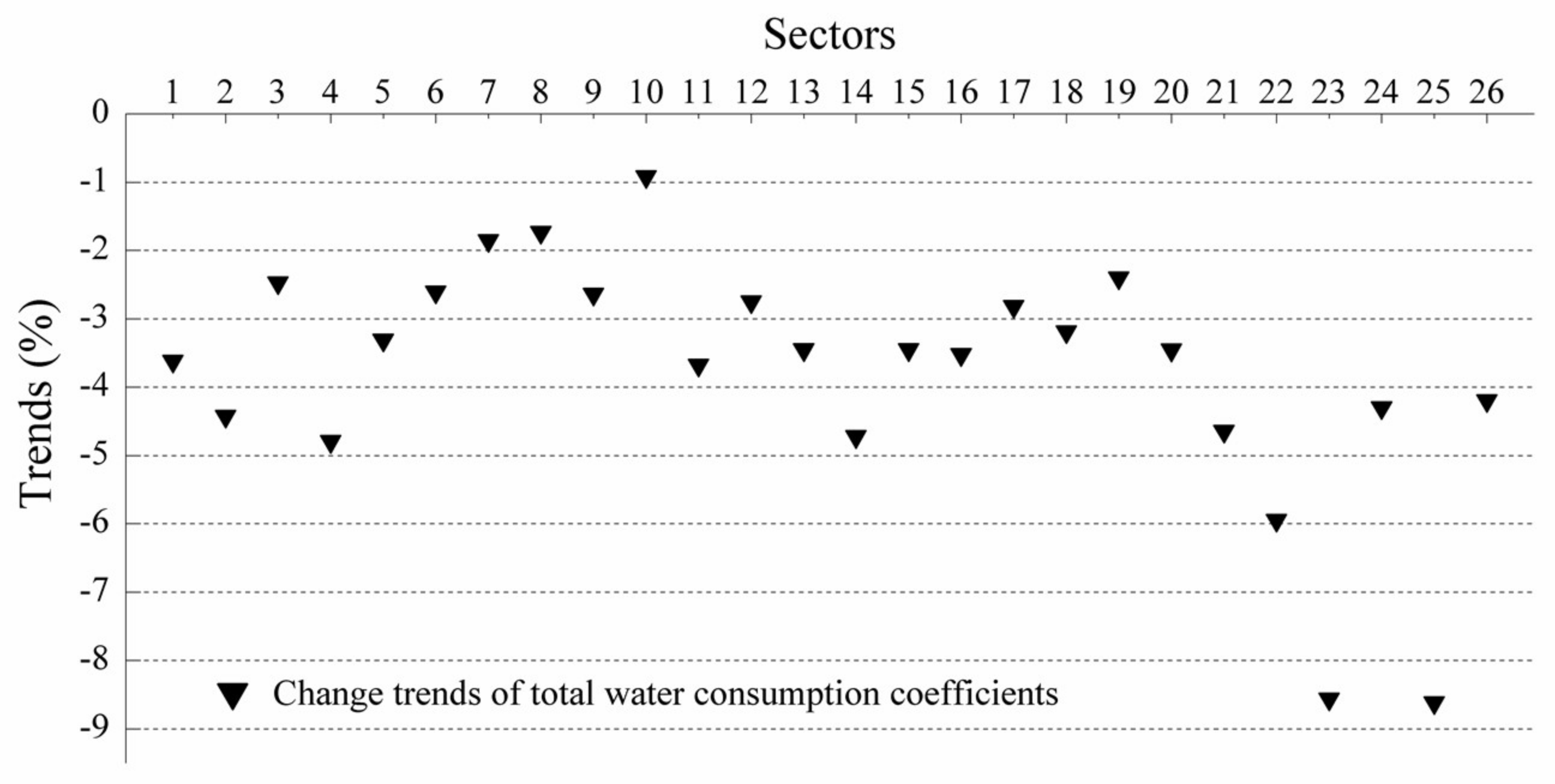
Virtual blue water footprint is determined by total water consumption coefficient and the corresponding expenditure. The expenditure reflects the consumption structure, while the total water consumption coefficient is related to the direct water consumption coefficient and industrial chain, thus reflecting the technological level and industrial structure. From 2002 to 2012, all the sectors had their total water consumption coefficients decreased, with the change rates ranging from −8.6% to −0.9% (Figure 4). Therein, the total water consumption coefficient in sector 25 (construction) decreased the most, of which the decrease rate was −8.6%. Therefore, the increase of $W{F}_{\mathrm{blue},\mathrm{virtual}}$ in most sectors was caused by the increase of domestic consumption. Especially, rural residents’ demands for sector 23 (gas production and supply) and urban residents’ demands for sector 11 (petroleum processing and coking) and sector 17 (transport equipment) expanded obviously during the study period.

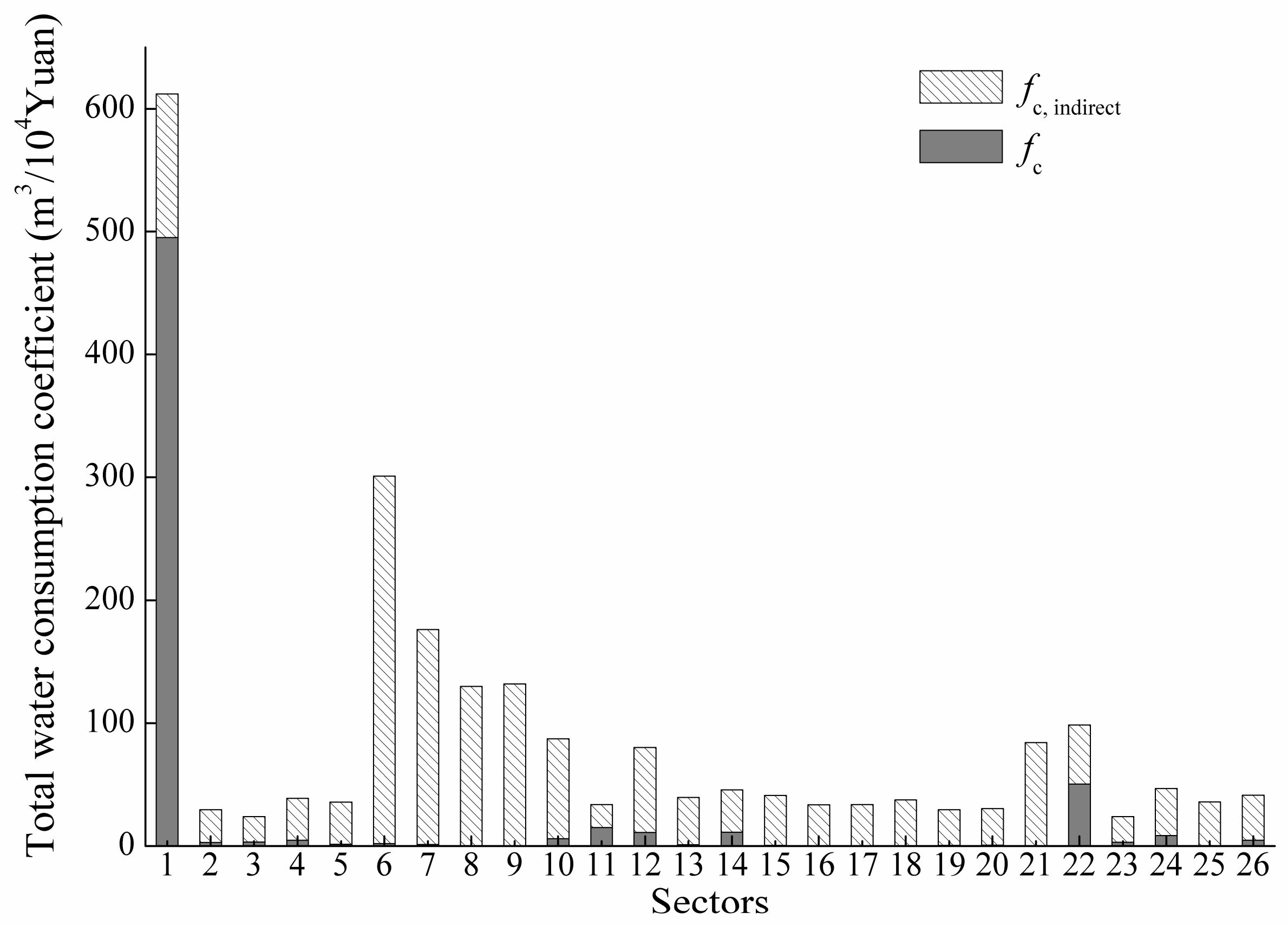
Taking the total water consumption coefficient in 2010 for example (Figure 4), we find that agriculture (sector 1) had the highest total water consumption coefficient, followed by food and tobacco processing (sector 6).

The compositions of total water consumption coefficients varied among sectors. Taking 2010 for example (Figure 5), the direct water consumption coefficient in agriculture accounted for the largest proportion of total water consumption coefficient, which reached 81%, followed by that in sector 22 (electronic and heating power production and supply) and that in sector 11 (petroleum processing and coking), of which the proportions were 51% and 44%, respectively. Sectors with the indirect water consumption coefficients higher than 50% reached 24, accounting for 92.3% of the total sectors; those higher than 90% reached 10, accounting for 38% of the total sectors, indicating that most of the virtual blue water footprint was produced by the intermediate virtual water input, i.e., the virtual water embedded in the raw materials, other than the fresh water input. In other words, the accumulated effect of industrial chain had very significant impacts on virtual blue water footprint.

3.3. The Consumption Structure of Grey Water Footprint

From 2002 to 2012, the average grey water caused by living return water was 0.72 trillion m³, and that caused by virtual return water was 2.89 trillion m³ (conversion with the Grade III water standard). Grey water footprint caused by virtual return water took a substantial proportion (80%) of grey water footprint, indicating that the consumption of goods and services for domestic consumption was the major way to produce grey water footprint.

Table 4. Sectoral virtual grey water footprint of China from 2002 to 2012. (Unit: million m³).

Sectors	2002	2005	2007	2010	2012	Average	Proportions	Trend
1	76,152	59,734	53,158	46,417	61,890	59,470	2.1%	−1.8%
2	1556	−3091	318	535	370	−63	0.0%	−18.4%
3	182	70	95	152	94	118	0.0%	−1.9%
4	46	2852	143	678	27	749	0.0%	−6.0%
5	114	−659	5	58	−40	−104	0.0%	−8.5%
6	656,596	1,044,654	543,475	589,357	546,162	676,049	23.7%	−2.4%
7	13,368	7823	5310	5191	7019	7742	0.3%	−4.8%
8	88,437	153,195	114,912	94,259	88,144	107,790	3.8%	−1.3%
9	21,379	10,149	20,339	13,147	17,615	16,526	0.6%	−0.7%
10	20,782	15,730	10,313	13,391	12,647	14,573	0.5%	−3.1%
11	1129	6274	1745	2348	4332	3166	0.1%	2.2%
12	77,256	13,142	44,466	41,800	46,023	44,538	1.6%	−1.9%
13	1700	1482	594	1155	371	1060	0.0%	−6.1%
14	105	−28	1516	2369	360	864	0.0%	7.3%
15	1570	−193	1645	1695	3805	1704	0.1%	13.5%
16	51,112	43,258	30,335	36,977	24,044	37,145	1.3%	−3.7%
17	10,588	16,624	19,627	52,281	28,268	25,478	0.9%	7.2%
18	3115	6525	8853	17,401	9509	9080	0.3%	6.6%
19	5168	5148	6215	11,183	5082	6559	0.2%	2.1%
20	426	1697	868	1814	548	1071	0.0%	0.8%
21	9668	8757	6803	9498	349	7015	0.2%	−5.2%
22	2019	1776	1288	2836	886	1761	0.1%	−1.5%
23	4147	20,933	6769	6946	1503	8059	0.3%	−5.0%
24	492	1316	680	2482	268	1048	0.0%	1.4%
25	1,009,117	309,151	515,587	3,366,144	0	1,040,000	36.4%	2.0%
26	798,105	828,593	763,382	723,146	822,375	787,120	27.5%	−0.2%

shows the sectoral virtual grey water footprint of China from 2002 to 2012. Virtual grey water footprint in tertiary industry (sector 26) was the highest (sector 25 was not taken into discussion since it does not indicate a specific industry), which was as high as 787.1 billion m³, accounting for 27.5% of the total $W{F}_{\mathrm{grey},\mathrm{virtual}}$, followed by that in sector 6 (food tobacco and processing), which was 676 billion m³, accounting for 23.7% of the total $W{F}_{\mathrm{grey},\mathrm{virtual}}$. Nineteen sectors had the proportions of $W{F}_{\mathrm{grey},\mathrm{virtual}}$ over total virtual grey water footprint less than one percent. As for change trends, seventeen sectors showed overall decreasing trends, with sector 2 (coal mining and processing) decreased the most, with the decrease rate of −18.4%. Sector 15 (metal products) had $W{F}_{\mathrm{grey},\mathrm{virtual}}$ increased the most, with the increase rate of 13.5%.

Virtual grey water footprint was caused by rural residents’ consumption (12%), urban residents’ consumption (33%), government consumption (11%), and gross fixed capital formation and inventory investment (44%).

Among the $W{F}_{\mathrm{grey},\mathrm{virtual}}$ caused by rural residents’ consumption (Table 3), sector 6 (food and tobacco processing) contributed the most, which was 181.7 billion m³ on average, accounting for 54.6% of the total $W{F}_{\mathrm{grey},\mathrm{virtual}}$ caused by rural residents’ consumption, followed by tertiary industry (sector 26), which contributed 88.1 billion m³ on average, accounting for 26.5%; twenty-one out of twenty-six sectors had very small $W{F}_{\mathrm{grey},\mathrm{virtual}}$ caused by rural residents’ consumption, accounting for less than one percent. As for change trends, sixteen out of twenty-six sectors showed decreasing trends. $W{F}_{\mathrm{grey},\mathrm{virtual}}$ caused by rural residents’ consumption in sector 5 (non-metallic and other minerals mining) and sector 14 (metal smelting and processing) presented the greatest and second greatest decreasing trends, with the decrease rates of −15.7% and −15.4%, respectively; while $W{F}_{\mathrm{grey},\mathrm{virtual}}$ caused by rural residents’ consumption in sector 23 (electronic and heating power production and supply) presented the greatest increasing trend, with the increase rate of 5.2%.

For the $W{F}_{\mathrm{grey},\mathrm{virtual}}$ caused by urban residents’ consumption, sector 6 (food and tobacco processing) also contributed the most, which was 416.8 billion m³ on average, accounting for 44.8% of the total $W{F}_{\mathrm{grey},\mathrm{virtual}}$ caused by urban residents’ consumption, followed by tertiary industry (sector 26), which contributed 312.8 billion m³ on average, accounting for 33.6%. As for change trends, seventeen out of twenty-six sectors showed decreasing trends. $W{F}_{\mathrm{grey},\mathrm{virtual}}$ caused by urban residents’ consumption in sector 3 (crude mining and processing), sector 5 (non-metallic and other minerals mining) and sector 14 (metal smelting and processing) showed the top three greatest decreasing trends, with the decrease rates of −20%, −15.8% and −15.4%, respectively; while $W{F}_{\mathrm{grey},\mathrm{virtual}}$ caused by urban residents’ consumption in sector 17 (transport equipment) and sector 11 (petroleum processing and coking) showed the greatest and second greatest increasing trends, with the increase rates of 10.2% and 9.9%, respectively.

For $W{F}_{\mathrm{grey},\mathrm{virtual}}$ caused by government consumption, it concentrated in tertiary industry (sector 26) and agriculture (sector 1), which were 307.5 billion m³ and 1.3 billion m³, accounting for 99.4% and 0.4% of the total $W{F}_{\mathrm{return},\mathrm{virtual}}$ caused by government consumption, respectively.

Virtual grey water footprint was determined by the conversion coefficient of grey water footprint, total return water coefficient and the corresponding expenditure. The expenditure reflects the consumption structure; total return water coefficient is related to the sectoral direct return water coefficient and industrial chain, thus reflecting the technological level and industrial structure; the conversion coefficient of grey water footprint is related to the pollutant concentration, water quality standard and background pollutant concentration, which reflects the production process, and the demands and status of environment quality.

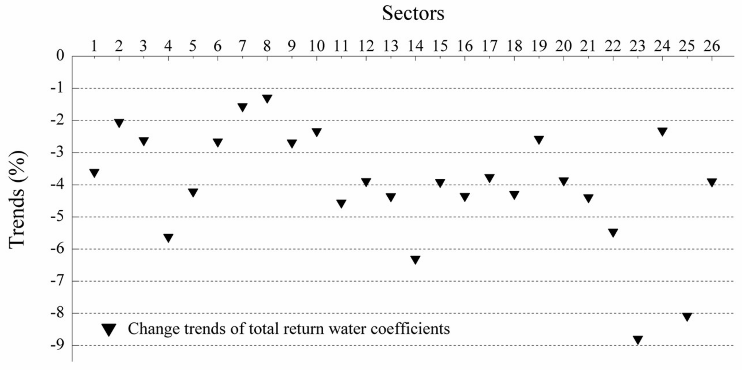
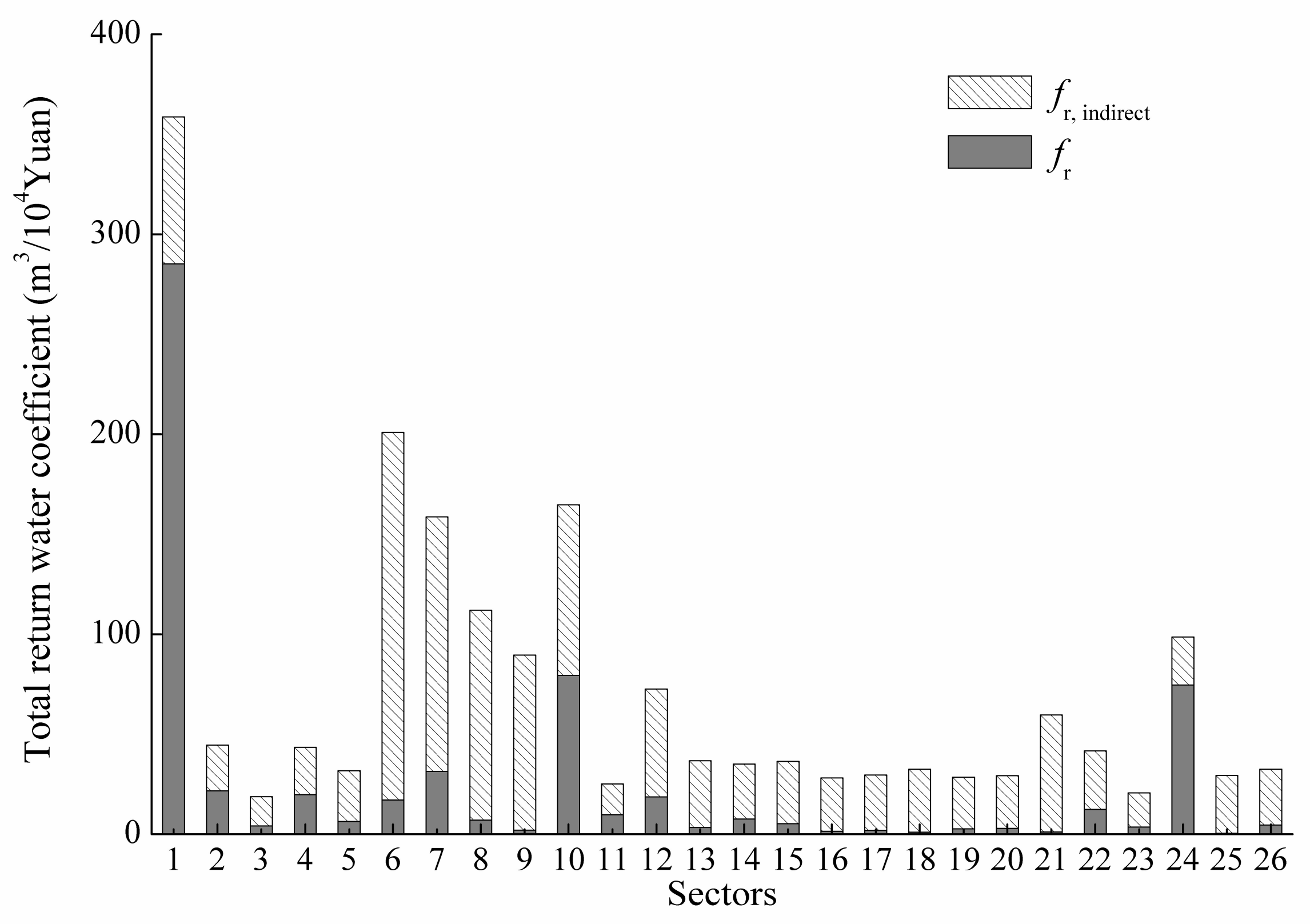
From 2002 to 2012, all sectors had the total return water coefficients decreased, with the decrease rates ranging from −8.8% to −1.3% (Figure 6). The contributions of direct return water coefficient to total return water coefficient varied among sectors. Taking total return water coefficient in 2010 for example (Figure 7), direct return water coefficient in agriculture (sector 1) contributed the greatest, accounting for 80%, followed by that in sector 24 (water production and supply), of which the proportion reached 76%. Sectors that had the proportions of indirect return water coefficient over total return water coefficient over 50% reached 24, accounting for 92% of the total sectors, those over 90% reached 11, accounting for 42% of the total sectors, indicating that most of the virtual return water was produced by the intermediate virtual return water input during the production, i.e., the virtual return water embedded in the raw materials, other than the direct return water. In other words, the accumulated effect of production chain had great impacts on grey water footprint.

Table 5. Change trends of conversion coefficients of sectoral virtual grey water footprint under Grade III water quality standard from 2002 to 2012.

Sectors	Trends	Sectors	Trends	Sectors	Trends	Sectors	Trends	Sectors	Trends
1	0.4%	7	−1.8%	13	−0.7%	19	1.5%	25	3.0%
2	−3.2%	8	−5.1%	14	1.3%	20	−0.1%	26	−1.7%
3	−4.3%	9	−6.8%	15	4.2%	21	−6.3%
4	−0.6%	10	−5.5%	16	−6.5%	22	0.4%
5	−5.9%	11	−5.5%	17	0.6%	23	−4.1%
6	−5.9%	12	−5.0%	18	1.6%	24	−4.1%

shows the change trends of conversion coefficients of sectoral virtual grey water footprint under Grade III water quality standard from 2002 to 2012. It is evident that from 2002 to 2012, most sectors had the conversion coefficients decreased, indicating a water quality improvement of return water during the study period. Therein, conversion coefficient in sector 3 decreased most, followed by that in sector 16 (general and specialized machinery).

Since both total return water coefficient and conversion coefficient of virtual grey water footprint mostly presented decreasing trends, while final demand exhibited an increasing trend as we discussed in Section 3.2, the conclusion is obvious that the decrease effect caused by total return water coefficients and conversion coefficients of virtual grey water footprint is more significant than the increase effect caused by final demand during the study period. Of particular importance, rural residents’ demands for sector 23 (gas production and supply) and urban residents’ demands for sector 11 (petroleum processing and coking) and sector 17 (transport equipment) expanded obviously during the study period.

3.4. External Water Footprint and Water Footprint Export

From 2002 to 2012, the average annual net virtual blue water export was 17.6 billion m³, and the average annual net virtual grey water export was 251.6 billion m³, implying China was a typical net virtual water export country, which was consistent with the result by Zhang et al. [26]. Figure 8 shows the compositions of water footprint export in China from 2002 to 2012. It is obvious that from 2007 to 2010, $W{F}_{\mathrm{export}}$ experienced a dramatic decrease due to the sharp decrease of $W{F}_{\mathrm{export},\mathrm{grey}}$. $W{F}_{\mathrm{export},\mathrm{grey}}$ dominated $W{F}_{\mathrm{export}}$ significantly. WSR and WEF from 2002 to 2012 (

Table 6. Water self-reliance and water export fraction in China from 2002 to 2012.

Year	2002	2005	2007	2010	2012
WSR	100%	100%	100%	100%	100%
WEF	6.7%	11.2%	10.3%	1.3%	6.5%

) indicate that, in terms of virtual water trade, China was self-reliant, the water used for producing the products and services to meet domestic consumption was taken domestically; meanwhile, China exported virtual water to other countries, which aggravated the water stress in China. Overall, China’s water stress is mainly from the water footprint produced by local consumption; water footprint export, especially after 2010, was relatively small.

4. Discussion

The average annual internal water footprint in China was 3.83 trillion m³ in this study, where the blue water footprint was 0.25 trillion m³, and the grey water footprint was 3.58 trillion m³. The internal water footprint is significantly higher and the blue water footprint is significantly lower than the 0.88 trillion m³ estimated by Hoekstra [27]. This is because on the one hand, we considered grey water footprint and distinguished water use and water consumption which Hoekstra did not; on the other hand, we did not consider the green water footprint that Hoekstra considered in calculating their agricultural water consumption. All these differences in data processing mean that the two estimates varied.

Different from blue water footprint and green water footprint, grey water footprint primarily focuses on the water quality variation. Many chemical substances can affect the water quality, so indicators for assessing water quality were various, and types and concentrations of pollutants also differed among different sectors. In this study, we choose NH₃-N and COD as the indexes to assess water quality because they were the most representative index in China’s water quality research. Concentration of background pollutants may also vary among different regions and can affect the estimation of grey water footprint, here we neglect the impact by considering the background pollution as zero. Besides, it is also subjective when we set the maximum allowable pollutant concentration. In this study, we refer to the maximum allowable pollutant concentration for Grade III of water quality defined by China Environmental Quality Standard for Surface Water (GB3838−2002). Based on the above analysis, our estimation of grey water footprint should be lower than the actual value.

5. Conclusions

By using input–output analysis and dilution theory, the internal water footprint, blue water footprint and grey water footprint of China from 2002 to 2012 were estimated, and the consumption structure of water footprint and virtual water trade were analyzed. Conclusions are as follows:

(1)

From 2002 to 2012, the average annual internal water footprint was 3.83 trillion m³ in China, in which grey water footprint took a large proportion of 93% on average. Both internal water footprint and grey water footprint experienced a decreasing trend from 2002 to 2012, except for a dramatic increase in 2010; while blue water footprint did not change significantly.

(2)

The annual average of blue water footprint was 0.25 trillion m³, in which the annual average of $W{F}_{\mathrm{blue},\mathrm{virtual}}$ was 0.22 trillion m³. $W{F}_{\mathrm{blue},\mathrm{virtual}}$ in agriculture (sector 1) was the largest among sectors, accounting for 39.2% of the total virtual blue water footprint. $W{F}_{\mathrm{blue},\mathrm{virtual}}$ in most sectors showed increased trends due to the increase of final demand.

(3)

The average grey water footprint caused by living return water was 0.72 trillion m³, and that caused by virtual return water was 2.14 trillion m³ (conversion with the Grade III water standard). Among sectors, annual $W{F}_{\mathrm{grey},\mathrm{virtual}}$ in tertiary industry (sector 26) was the highest, which accounted for 27.5% of the total $W{F}_{\mathrm{grey},\mathrm{virtual}}$, followed by that in food and tobacco processing (sector 6). $W{F}_{\mathrm{grey},\mathrm{virtual}}$ in most sectors showed decreasing trends due to the decreases of total return water coefficients and conversion coefficients of virtual grey water footprint.

(4)

For water resources, China was self-reliant, the water used for producing the products and services to meet domestic consumption was taken domestically; meanwhile, China exported virtual water to other countries, which aggravated the water stress in China.

References

- Hoekstra, A.Y. Human appropriation of natural capital: A comparison of ecological footprint and water footprint analysis. Ecol. Econ. 2009, 68, 1963–1974. [Google Scholar] [CrossRef]
- Falkenmark, M.; Rockstrom, J. The new blue and green water paradigm: Breaking new ground for water resources planning and management. J. Water Resour. Plan. Manag. 2006, 132, 129–132. [Google Scholar] [CrossRef]
- Feng, K.; Siu, Y.L.; Guan, D.; Hubacek, K. Assessing regional virtual water flows and water footprints in the Yellow River Basin, China: A consumption based approach. Appl. Geogr. 2012, 32, 691–701. [Google Scholar] [CrossRef]
- Yang, H.; Wang, L.; Zehnder, A.J.B. Water scarcity and food trade in the Southern and Eastern Mediterranean countries. Food Policy 2007, 32, 585–605. [Google Scholar] [CrossRef]
- Zhang, Z.; Shi, M.; Yang, H. Understanding Beijing’s water challenge: A decomposition analysis of changes in Beijing’s water footprint between 1997 and 2007. Environ. Sci. Technol. 2012, 46, 12373–12380. [Google Scholar] [CrossRef] [PubMed]
- Zhao, X.; Yang, H.; Yang, Z.; Chen, B.; Qin, Y. Applying the input-output method to account for water footprint and virtual water trade in the Haihe River basin in China. Environ. Sci. Technol. 2010, 44, 9150–9156. [Google Scholar] [CrossRef] [PubMed]
- Hoekstra, A.Y.; Chapagain, A.K. Water footprints of nations: Water use by people as a function of their consumption pattern. Water Resour. Manag. 2006, 21, 35–48. [Google Scholar] [CrossRef]
- Hoekstra, A.Y.; Chapagain, A.K.; Aldaya, M.M.; Mekonnen, M.M. The Water Footprint Manual, State of the Art 2009; Water Footprint Network: Enschede, The Netherlands, 2009. [Google Scholar]
- Munoz Castillo, R.; Feng, K.; Hubacek, K.; Sun, L.; Guilhoto, J.; Miralles-Wilhelm, F. Uncovering the Green, Blue, and Grey Water Footprint and Virtual Water of Biofuel Production in Brazil: A Nexus Perspective. Sustainability 2017, 9, 2049. [Google Scholar] [CrossRef]
- Zhao, D.D.; Tang, Y.; Liu, J.G.; Tillotson, M.R. Water footprint of Jing-Jin-Ji urban agglomeration in China. J. Clean. Prod. 2017, 167, 919–928. [Google Scholar] [CrossRef]
- Wang, Z.; Huang, K.; Yang, S.; Yu, Y. An input-output approach to evaluate the water footprint and virtual water trade of Beijing, China. J. Clean. Prod. 2013, 42, 172–179. [Google Scholar] [CrossRef]
- Zhao, X.; Chen, B.; Yang, Z.F. National water footprint in an input-output framework—A case study of China 2002. Ecol. Model. 2009, 220, 245–253. [Google Scholar] [CrossRef]
- Zhang, Z.; Shi, M.; Yang, H.; Chapagain, A. An Input-Output Analysis of Trends in Virtual Water Trade and the Impact on Water Resources and Uses in China. Econ. Syst. Res. 2011, 23, 431–446. [Google Scholar] [CrossRef]
- Kang, J.; Lin, J.; Cui, S.; Li, X. Water footprint of Xiamen city from production and consumption perspectives (2001–2012). Water Sci. Technol. 2017, 17, 472–479. [Google Scholar] [CrossRef]
- Daniels, P.L.; Lenzen, M.; Kenway, S.J. The Ins and Outs of Water Use—A Review of Multi-Region Input-Output Analysis and Water Footprints for Regional Sustainability Analysis and Policy. Econ. Syst. Res. 2011, 23, 353–370. [Google Scholar] [CrossRef]
- Sun, Y.; Shen, L.; Lu, C. Study on the water footprint and external water dependency of Beijing. Water Sci. Technol. 2016, 16, 1077–1085. [Google Scholar] [CrossRef]
- Ridoutt, B.G.; Pfister, S. A revised approach to water footprinting to make transparent the impacts of consumption and production on global freshwater scarcity. Glob. Environ. Chang. 2010, 20, 113–120. [Google Scholar] [CrossRef]
- Zhao, X.; Liu, J.; Liu, Q.; Tillotson, M.R.; Guan, D.; Hubacek, K. Physical and virtual water transfers for regional water stress alleviation in China. Proc. Natl. Acad. Sci. USA 2015, 112, 1031–1035. [Google Scholar] [CrossRef] [PubMed]
- Hoekstra, A.Y.; Hung, P.Q. Globalisation of water resources: International virtual water flows in relation to crop trade. Glob. Environ. Chang. 2005, 15, 45–56. [Google Scholar] [CrossRef]
- Yang, H.; Wang, L.; Abbaspour, K.C.; Zehnder, A.J.B. Virtual water trade: An assessment of water use efficiency in the international food trade. Hydrol. Earth Syst. Sci. 2006, 10, 443–454. [Google Scholar] [CrossRef]
- Hoekstra, A.Y.; Mekonnen, M.M. The water footprint of humanity. Proc. Natl. Acad. Sci. USA 2012, 109, 3232–3237. [Google Scholar] [CrossRef] [PubMed]
- Liu, W.; Antonelli, M.; Liu, X.; Yang, H. Towards improvement of grey water footprint assessment: With an illustration for global maize cultivation. J. Clean. Prod. 2017, 147, 1–9. [Google Scholar] [CrossRef]
- Zeng, Z.; Liu, J.; Savenije, H.H.G. A simple approach to assess water scarcity integrating water quantity and quality. Ecol. Indic. 2013, 34, 441–449. [Google Scholar] [CrossRef]
- Sun, C.Z.; Han, Q.; Deng, D.F. The spatial correlation of the provincial grey water footprint and its loading coefficient in China. Acta Ecol. Sin. 2016, 36, 86–97. [Google Scholar]
- Van Oel, P.R.; Mekonnen, M.M.; Hoekstra, A.Y. The external water footprint of the Netherlands: Geographically-explicit quantification and impact assessment. Ecol. Econ. 2009, 69, 82–92. [Google Scholar] [CrossRef]
- Zhang, Z.; Yang, H.; Shi, M. Spatial and sectoral characteristics of China’s international and interregional virtual water flows—Based on multi-regional input–output model. Econ. Syst. Res. 2016, 28, 362–382. [Google Scholar] [CrossRef]
- Hoekstra, A.Y.; Chapagain, A.K. Globalization of Water: Sharing the Planets Freshwater Resources; Blackwell: Oxford, UK, 2008. [Google Scholar]
Figure 1.
Calculation flow chart. WF: Water footprint; NVBWI/NVGWI: Net virtual blue/grey water import; TNVBWI/TNVGWI: Total net virtual blue/grey water import; k: Conversion coefficient of grey water footprint; Vc/Vr: Water consumption/Return water; rc/rr: Total water consumption coefficient/Total return water coefficient; P: Expenditure.
Figure 2.
Internal water footprint (WF) of China from 2002 to 2012.
Figure 3.
Blue water footprint of China from 2002 to 2012.
Figure 4.
Change trends of total water consumption coefficients from 2002 to 2012.
Figure 5.
Total water consumption coefficients of different sectors in 2010.
Figure 6.
Change trends of total return water coefficients from 2002 to 2012.
Figure 7.
Total return water coefficients of different sectors in 2010.
Figure 8.
Compositions of water footprint export of China from 2002 to 2012.