Improvement of Two Evapotranspiration Estimation Models Using a Linear Spectral Mixture Model over a Small Agricultural Watershed

Abstract

Accurately measuring regional evapotranspiration (ET) is of great significance for studying global climate change, regional hydrological cycles, and surface energy balance. However, estimating regional ET from mixed vegetation types is still challenging. In this study, the Surface Energy Balance Algorithm for Land (SEBAL) and the Surface Energy Balance System (SEBS) models were applied to estimate surface ET in a small agricultural watershed. Landsat8 satellite images were used as input data to the single-source models. The two models were validated at single point and ecosystem scales. The results showed that both models overestimated ET observations in paddy fields and orange groves but underestimated them in dry farmland. The error was mainly caused by the heterogeneity of the mixed pixels. The linear spectral mixture model and a set of equations were introduced to reduce the simulation error. The revised results showed that the relative precision of SEBAL was improved by 9.87% and 10.06%, respectively. This research is expected to provide new ideas for future development of accurate remote-sensing ET estimations on heterogeneous surfaces.

1. Introduction

Evapotranspiration (ET) is a major component of global hydrological cycles and provides an important nexus between terrestrial water, carbon and surface energy exchange. In addition, ET is inherently difficult to measure and estimate, especially on large spatial scales. Obtaining accurate ET estimates has great significance for understanding regional hydrological cycles and energy balance. Currently, the global water resource situation is becoming more and more serious, and the importance of water resources is becoming increasingly significant. Therefore, the constantly increasing requests for quantitative management of water resource demand have prompted further research on ET estimation.

Traditional methods for estimating ET include the evaporating dish and the Lysimeter [1]. These methods are applicable on a field scale, while the development of remote-sensing technology and the continuous improvement of satellite image resolution provide a reliable guarantee for obtaining periodic regional surface ET values in a timely manner. Unlike traditional methods which estimate ET directly, the remote sensing method calculates ET step-by-step using various inversion algorithms. In recent decades, a large number of remote-sensing regional ET models have been developed and applied. The first type of model is the statistical empirical models which establish relationships between site meteorological observations and ET data associated with remote-sensing parameters (vegetation index, surface temperature, soil moisture) and expand relationships to describe regional ET [2,3,4]. The second type of model is the single-source energy balance models: the Surface Energy Balance Index [5], the Surface Energy Balance Algorithm for Land (SEBAL [6,7,8,9]); the Surface Energy Balance System (SEBS [10]); the Simplified Surface Energy Balance Index [11], and Mapping ET with Internalized Calibration [12]. The third type of model is the two-source energy balance models that distinguish soil and vegetation contributions, including the S-W model [13], the N95 model [14], and the Atmosphere–Land Exchange Inverse model [15].

Among these models, SEBAL and SEBS have been widely used in various countries around the world by many researchers [16,17,18,19,20]. ET is estimated from a single measurement point and then expanded to a regional scale using SEBAL and SEBS. These models break through the limitations of traditional methods, provide a new way of estimating regional ET, and ensure high estimation accuracy. Therefore, remote-sensing methods have an irreplaceable role in estimating ET at the regional scale [21]. Taking advantage of remote-sensing technology to estimate ET and analyze its spatial variation characteristics at the regional scale has far-reaching significance for studying climate change, maintaining balanced ecosystems, and ensuring acceptable utilization efficiency for regional water resources.

Current research is focused on estimating overall ET at the large regional scale. However, it has overlooked the estimation error from mixed pixels of different crop types that occurs at the regional scale, leading to less-than-precise estimations [18,22,23,24]. Freund et al. [25] concluded that averaging over spatial heterogeneity leads to overestimation of ET in large scale Earth system models. Byun et al. [26] also found that SEBS overestimated trends in the estimation of latent heat flux over heterogeneous surfaces in cropland and mixed forest. Surface heterogeneity brings error to regional ET estimation and has greatly restricted the estimation accuracy of single-pixel vegetation ET at the regional scale [27,28].

The objective of this study was to eliminate/reduce this estimation error and to improve the estimation accuracy. Therefore, this paper will focus on single-source model application and the resulting improvements. A small watershed in typical Southern hilly farmland located in Jiangxi Province, China was chosen for this study. Bowen ratio energy balance system, Automatic Weather Station (AWS) and large aperture scintillometer (LAS) observations were used for comparative verification with SEBAL and SEBS at single-point and ecosystem scales. In combination with land-cover type maps of 30 m and 0.5 m resolution, surface evaporation was analyzed under various land-cover types. Finally, the linear spectral mixture model (LSMM) was used to resolve the remote-sensing ET estimation error of mixed pixels at the ecosystem scale in the two models. It is expected that this study will provide new ideas for the future development of remote-sensing ET models. These research results could help people to monitor the water situation of different crops in small agricultural watersheds in a timely and accurate manner, provide scientific evidence to guide crop irrigation, and support management and evaluation of regional water resources.

2. Materials

2.1. Study Area

The study area is a core experimental area (5.5 km × 5.5 km) in a small Sunjia watershed, and is located on the Liujiazhan reclamation farm, Yujiang County, Yingtan City, Jiangxi Province (116°55′ E, 28°15′ N), about 4 km from the Chinese Academy of Red Soil Ecological Experimental Station. The Liujiazhan reclamation farm is composed of low, hilly, red soil, with a surface elevation of 38~55 m above sea level, slowly varying terrain, and a slope of less than 8°. There are three vegetation types in the observation area: double-cropped rice, peanut/sweet potato rotation, and orange groves.

The study area has a subtropical monsoon climate with an average annual precipitation of 1795 mm, and an ET of 1318 mm. The average annual temperature is 18.4 °C, and sunshine duration is 1739.9 h. The rainy season (April–June) accounts for about 50 percent of annual precipitation. ET from July to September is nearly 50 percent of the annual amount.

2.2. Ground Measurements

In the study area, meteorological measurements were taken at two national meteorological stations and three HOBO U-30 (ONSET Inc., Folsom, CA, USA) automatic weather stations (air temperature, precipitation, land-surface temperature, atmospheric pressure, wind speed, relative humidity, sunshine duration, and solar radiation) at a height of 2 m above the ground. ET data at the site scale were obtained by the Bowen ratio energy balance system (Campbell Scientific Inc., Logan, UT, USA), and the vertical gradient observations were 1.5 m and 3 m. Automatic weather stations and Bowen ratio energy balance systems were set up on three different crop types (location are shown in Figure 1c). Regional ET data were obtained by a large-aperture scintillometer (LAS, Kipp & Zonen Inc., Delft, The Netherlands). The LAS effective height was 9 m, and the spatial interval between the transmitter and receiver was 840 m (Figure 1c). Soil heat flux was measured by three soil heat flux plates (HFP-01, Hukse Flux, Delft, The Netherlands) buried in the soil at a depth of 5 cm at the same location as the Bowen ratio energy balance system. Observations were taken every 15 min, on average. The flux contribution source area of LAS was estimated by the footprint model [29,30]. The footprint function can be expressed as

$$f_{LAS}={\displaystyle {\int }_{x_2}^{x_1}{W}_{\left(\mathrm{x}\right)}}f\left(x-x^{\prime },y-y^{\prime },{\mathrm{z}}_{LAS}\right)dx$$

(1)

$$W_{\left(x\right)}=4{\pi }^2{\upsilon }_{LAS}^2{\displaystyle {\int }_0^{\infty }\upsilon \varphi \left(\upsilon \right)}{\sin }^2\left[\frac{{\upsilon }^{2}x(d-x)}{2{\upsilon }_{LAS}d}\right]\times {\left[\frac{2J_1\left(0.5\upsilon D\frac{x}{d}\right)}{0.5\upsilon D\frac{x}{d}}\times \frac{2J_1\left(0.5\upsilon D\left(1-\frac{x}{d}\right)\right)}{0.5\upsilon D\left(1-\frac{x}{d}\right)}\right]}^{2}d\upsilon$$

(2)

where f_LAS is the footprint function, x₁ and x₂ are the positions of the transmitter and receiver, x and y are the propagation distances along the LAS path (m), x’ and y’ are the coordinates of each point in the upwind direction over the LAS path, Z_LAS is the effective measurement height (m), W_(x) is the weight function over the LAS path, d is the path length (m), ${\upsilon }_{LAS}$ is the optical wave number, υ is the turbulence spatial spectrum wave number, D is the aperture diameter of LAS, ϕ(υ) is the three-dimensional spectrum of refractive index fluctuations ($0.033{\upsilon }^{\frac{-11}{3}}$), and J₁(m) is the Bessel function of the first kind of order one.

The LAS resolution of the source area was 30 m, and the date of the footprint weight map was on Day Of Year (DOY) 284, 2015 (encompassing 90% of the flux contribution), as shown in Figure 1c.

2.3. Remote-Sensing Data

The remote-sensing datasets used in this study were derived from Landsat8 data. The input data for SEBAL and SEBS were obtained by clipping a 5.5 km × 5.5 km image for the study area. The used data time is shown in

Table 1. Day of Years (DOYs) of remote-sensing images used in this study.

Year	DOY
2013	134, 182, 214, 278
2014	073, 121, 217, 281, 291
2015	252, 284 *

Note: Images marked with * was the input image used to extract the abundance.

.

The Landsat8 satellite was launched on 11 February 2013, and images the entire Earth’s surface every 16 days. Landsat 8 carries two instruments: OLI (Operational Land Imager) and TIRS (Thermal Infrared Sensor). The OLI consists of nine spectral bands with a spatial resolution of 15 m for panchromatic bands and 30 m spatial resolution for multispectral bands. The approximate scene size is a 185 km cross-track field of view. The TIRS provides two thermal bands; the two bands complement each other and effectively separate surface and atmospheric temperatures as well as compensating for atmospheric effects. The TIRS radiation resolution is higher than the original resolution. The two thermal bands were collected at 100 m but were resampled at 30 m to match the OLI multispectral bands. Landsat8 can provide reliable data for research and applications in agriculture, water resources, forest, urban planning, and environmental studies.

The classification of land-cover types in the study area was based on Pleiades satellite data with a resolution of 0.5 m. Pleiades is a follow-on satellite of SPOT and is composed of Pleiades-1A and Pleiades-1B, two very high-resolution optical Earth-imaging satellites. Pleiades-1A and Pleiades-1B were launched on 17 December 2011 and 2 December 2012, respectively. The Pleiades provide coverage of Earth’s surface with a repeat cycle of 26 days. The Pleiades consist of five spectral bands with spatial resolution of 0.5 m for panchromatic bands and 2 m spatial resolution for the multispectral bands, with a 20-km swath. On one hand, the Pleiades maintain the band set and stereo imaging characteristics of SPOT; on the other hand, they were redesigned for the spatial resolution, observational flexibility, and data acquisition method. Currently, Pleiades is one of a number of Earth observation satellites that offers a high level of technology, observational precision, and timeliness.

3. Methods

3.1. Theoretical Basis of SEBAL

SEBAL, proposed by Bastiaanssen et al. [7,8], is a typical single-source ET model based on the surface energy balance equation. The model is featured in the minimum requirements for near-surface meteorological measurements. There are three steps to compute ET in SEBAL. First, relevant surface parameters (albedo, vegetation index, emissivity, surface temperature) are derived from remote-sensing data under sunny weather conditions. Second, net radiation flux and soil heat flux at the ecosystem scale are computed by combining the surface parameters with the corresponding surface meteorological observation data (air temperature, wind speed, average vegetation height). Third, both sensible and latent heat flux are estimated using the linear relationship between surface temperature and the air–temperature difference between hot and cold pixels within the remote-sensing image, as well as iterative computations, according to the Monin–Obukhov similarity theory. For details of the theory, parameter inputs, and calculations, please refer to Bastiaanssen et al. [6,7,8,9].

3.1.1. Soil Heat Flux in SEBAL

Soil heat flux is the change in heat storage in soil and vegetation due to conduction. In SEBAL, Bastiaanssen’s [9] empirical parametric equation is used to consider the surface albedo, the vegetation index, and the land-surface temperature:

$$G=\frac{T_s-273.15}{\alpha }\left(0.0038\alpha +0.0074{\alpha }^2\right)\left(1-0.98NDV{I}^4\right)R_n$$

(3a)

$$G=0.41R_n-51$$

(3b)

$$G=0.3R_n$$

(3c)

where G is the soil heat flux, R_n is the surface net radiation flux, T_s is the land surface temperature (°C), α is the surface albedo, and NDVI is the Normalized Difference Vegetation Index. Formula (3a) is suitable for vegetated areas, (3b) is suitable for water bodies, and (3c) is suitable for urban bare land.

3.1.2. Sensible Heat Flux in SEBAL

Sensible heat flux is the heat loss/gain to the air by convection due to a temperature difference. The SEBAL model computes sensible heat flux using the following equation:

$$\mathrm{H}=\frac{\rho \times C_p\times dT}{{\mathrm{r}}_{\mathrm{ah}}}$$

(4)

$$r_{ah}=\frac{\ln \left(\frac{{\mathrm{z}}_2}{{\mathrm{z}}_1}\right)-{\psi }_{h\left({\mathrm{z}}_2\right)}+{\psi }_{h\left({\mathrm{z}}_1\right)}}{k^2{u}_{200}}\left[\ln \left(\frac{200}{{\mathrm{z}}_{0m}}\right)-{\psi }_{m(200)}\right]$$

(5)

where $\rho$ is the air density (kg/m³), $C_p$ is the specific heat of air at a constant pressure (1004 J/kg/K), $dT$ is the air temperature difference (T₁ − T₂) (K) between heights ${\mathrm{z}}_1$ and ${\mathrm{z}}_2$, $r_{ah}$ is the aerodynamic resistance (s/m), $u_{200}$ is the wind speed at the blending height (assumed to be 200 m above the ground), $k$ is the Karman constant (0.41), ${\mathrm{z}}_{0m}$ is the surface momentum roughness length for each pixel, ${\psi }_{m(200)}$ is the stability correction function for momentum at 200 m, ${\mathrm{z}}_2$ is 2 m, ${\mathrm{z}}_1$ is 0.1 m, and ${\psi }_{h\left({\mathrm{z}}_2\right)}$ and ${\psi }_{h\left({\mathrm{z}}_1\right)}$ are the stability correction functions for heat transfer at 2 m and 1 m respectively.

In SEBAL, the surface momentum and thermal roughness lengths for each pixel can be calculated by two methods [9]:

$${\mathrm{z}}_{0m}=\exp [(a\times NDVI/\alpha )+b]$$

(6)

$${\mathrm{z}}_{0h}={\mathrm{z}}_{0m}/\exp \left(k{B}^{-1}\right)$$

(7)

where a and b are correlation constants that can be derived from the NDVI and the surface albedo (α) fitted to multiple pixels in the study area. The surface albedo can help to achieve a better distinction between vegetation pixels at different heights that have similar NDVI. Z_0h is the thermal roughness length. kB⁻¹ is an area constant (2.3) in SEBAL.

The SEBAL model computes dT for each pixel by assuming a linear relationship between dT and T_s:

$$dT=a{T}_s+b$$

(8)

where a, b are the correlation coefficients in the SEBAL calculation that chooses cold and hot “anchor” pixels.

SEBAL determines the boundary conditions (zero ET and maximum ET) of the surface energy balance based on hot and cold pixels. Cold pixels are generally selected from well-watered and fully covered agricultural fields, such as paddy fields. They are assumed to have approximately constant near-surface air temperatures and surface temperatures. However, water bodies cannot be chosen as cold pixels, because the soil heat flux in water is greater than that on land. Hot pixels are generally selected from dry and bare agricultural fields where it is assumed that no ET taking place. Both cold and hot pixels must be selected from a uniform surface to reduce errors caused by mixed pixels.

When a wet paddy field is chosen as the cold pixel source, the ET rate is usually about 5% larger than the reference ET. Therefore, the sensible heat flux in cold pixels can be expressed as

$$H_{cold}=R_n-G-1.05\lambda E{T}_r.$$

(9)

If no precipitation has occurred within the four days prior to the image date, then ET_hot is assumed to be zero for a hot (dry) agricultural field having no green vegetation and with a dry soil surface layer. Therefore, the sensible heat flux in hot pixels can be expressed as H_hot = R_n − G. Hence, dT_cold and dT_hot can be determined by

$$d{T}_{cold}=H_{cold}\times r_{ah\_cold}/\left({\rho }_{cold}\times C_p\right),d{T}_{hot}=H_{hot}\times r_{ah\_hot}/\left({\rho }_{hot}\times C_p\right)$$

(10)

and the coefficients a and b can be obtained by

$$a=\frac{d{T}_{hot}-d{T}_{cold}}{T_{hot}-T_{cold}},b=\frac{d{T}_{cold}{T}_{hot}-d{T}_{hot}{T}_{cold}}{T_{hot}-T_{cold}}.$$

(11)

3.1.3. Daily ET in SEBAL

In SEBAL, the latent heat flux is obtained as follows:

λET = R_n − G − H

(12)

where λET is the instantaneous latent heat flux (w/m²).

The hourly ET can be calculated by integrating the instantaneous values of the latent heat fluxes and transforming them in mm/h.

The evaporative fraction (hourly ET/hourly reference ET) is assumed to be constant over a 24 h period. Therefore, daily ET can be calculated by

$$E{T}_{\mathrm{daily}}=\mathsf{\Lambda }\times E{T}_{r\_\mathrm{daily}}$$

(13)

where Λ is the evaporative fraction, and ET_{r_dalily} is the daily reference ET.

3.2. Theoretical Basis of SEBS

SEBS, proposed by Su [10], is an improved version of SEBAL. The model has an improved surface roughness length algorithm for heat and is more adaptable for regional-scale applications and has become more popular [10,31].

SEBS consists of three main modules: (1) SEBAL which uses remote-sensing data to calculate ET; (2) a new algorithm for kB⁻¹ in which the kB⁻¹ scheme proposed by Menenti and Choudhury [5] is used for the fully vegetated area, while the kB⁻¹ scheme proposed by Brutsaert [32] is used for bare soil. A new calculation method for the kB⁻¹ coefficients was applied to accommodate the incomplete vegetation coverage and to more accurately estimate surface roughness length for heat. (3) The measurement height is determined to be either in the atmospheric surface layer (ASL) or in the planetary boundary layer (PBL) based on the height obtained using the Monin–Obukhov Similarity (MOS) theory [33] and the Bulk Atmospheric Boundary Layer Similarity (BAS) theory [32]. For details of the particular theory and input requirements of SEBS, please refer to Su [10].

3.2.1. Soil Heat Flux in SEBS

In SEBS, the soil heat flux is calculated using a relationship between vegetation coverage and net radiation flux:

$${\mathrm{G}=\mathrm{R}}_n\left[{\mathsf{\Gamma }}_c+\left({\mathsf{\Gamma }}_s-{\mathsf{\Gamma }}_c\right)\left(1-f_c\right)\right]$$

(14)

where Γ_c is the soil heat flux ratio for a fully vegetated area, Γ_s is the ground heat flux ratio for bare soil, and f_c is the vegetation fraction. In this study, Γ_c = 0.05 [34], and Γ_s = 0.315 [3].

3.2.2. Sensible Heat Flux in SEBS

Sensible heat flux in SEBS is computed by the following equations:

$$u=\frac{u_{\ast }}{k}\left[\ln \left(\frac{\mathrm{z}-d_0}{{\mathrm{z}}_{0m}}\right)-{\psi }_m\left(\frac{\mathrm{z}-d_0}{L}\right)+{\psi }_m\left(\frac{{\mathrm{z}}_{0m}}{L}\right)\right],$$

(15)

$$L=-\frac{\rho C_p{u}_{\ast }^3{\theta }_v}{kg\mathrm{H}},$$

(16)

$$H=k{u}_{\ast }\rho C_p({\theta }_0-{\theta }_a){\left[\ln \left(\frac{\mathrm{z}-d_0}{{\mathrm{z}}_{0h}}\right)-{\psi }_h\left(\frac{\mathrm{z}-d_0}{L}\right)+{\psi }_h\left(\frac{{\mathrm{z}}_{0h}}{L}\right)\right]}^{-1},$$

(17)

where z is the height above the surface (m), u is the wind speed (m/s), u* is the friction velocity (m/s), ρ is the air density (kg/m³), k is the Karman constant (0.41), d₀ is the zero plane displacement (m), Z_0m is the roughness length for momentum, Z_0h is the roughness length for heat, θ₀ and θ_a are the potential temperatures at the surface and at height z, respectively (K), Ψ_m and Ψ_h are the stability correction factors for sensible heat and momentum transfer, respectively, g is the acceleration due to gravity (m/s), C_p is the specific heat of air at a constant pressure (1004 J/kg/K), H is the sensible heat flux (W/m²), L is the Obukhov length (m), and θ_v is the potential virtual temperature near the surface (K).

The roughness length for heat (Z_0h) varies with land-cover type, atmospheric circulation, and surface thermodynamic characteristics. Based on the work of Massman [35], Su [31] proposed a simple model for the roughness length for heat and an extended model for the residual impedance kB⁻¹:

$${\mathrm{z}}_{0\mathrm{m}}=0.005+0.5{\left[\frac{NDVI}{NDV{I}_{\max }}\right]}^{2.5},$$

(18)

$${\mathrm{z}}_{0h}={\mathrm{z}}_{0m}/\exp \left(k{B}^{-1}\right),$$

(19)

$$k{B}^{-1}=\frac{k{C}_d}{4C_t\frac{u_{\ast }}{u\left(h\right)}(1-e^{-nec/2})}{f}_c^2+2f_c{f}_s\frac{k•\frac{u_{\ast }}{u\left(h\right)}•\frac{{\mathrm{z}}_{0m}}{h}}{C_t^{\ast }}+k{B}_s^{-1}{f}_s^2,$$

(20)

where f_c is the fractional canopy coverage, f_s = 1 − f_c, C_d is the vegetation drag coefficient (0.2), C_t is the heat transfer coefficient of leaves (0.01), C_t^* is the heat transfer coefficient of soil, n_ec is the within-canopy wind speed profile extinction coefficient, u* is the friction velocity, u(h) is the horizontal wind speed at the canopy top. The roughness Reynolds number Re* = h_su*/ν was also proposed, where h_s is the roughness length of the soil and ν is the kinematic viscosity of the air.

3.2.3. Daily ET in SEBS

In SEBS, the estimation of the relative evaporative fraction considers the limiting case in dryness and wetness using Equation (23). In the case of extremely dry surfaces, H reaches its maximum and ET approaches zero, due to the lack of soil moisture. In the case of extremely wet surfaces, ET reaches its potential rate. The relative evaporative fraction is determined by the following equation:

$${\mathsf{\Lambda }}_r=1-\frac{H-H_{wet}}{H_{dry}-H_{wet}}.$$

(21)

The evaporative fraction is expressed as the ratio of ET to available energy at the surface (R_n − G), as follows:

$$\mathsf{\Lambda }=\frac{\lambda E}{H+\lambda E}=\frac{\lambda E}{R_n-G}=\frac{{\mathsf{\Lambda }}_r\times \lambda E_{wet}}{R_n-G}.$$

(22)

When the evaporative fraction is determined, daily ET can be inferred as follows:

$$E{T}_{daily}=8.64\times {10}^7\times \underset{0}{\overset{24}{\mathsf{\Lambda }}}\times \frac{\overline{R_n}-\overline{G_0}}{{\lambda }_{\rho w}}$$

(23)

where ET_daily is the daily ET(mm·d⁻¹), $\underset{0}{\overset{24}{\mathsf{\Lambda }}}$ is the mean daily evaporative fraction estimated by the evaporation ratio constant principle [13], $\overline{R_n}$ and $\overline{G_0}$ are the mean daily net radiation and mean daily soil heat fluxes.

3.3. Theoretical Basis of LSMM

Though SEBAL and SEBS have been widely used, these two energy balance models have also showed some poor performances in areas with mixed vegetation types at the regional scale. There are many sources of error in SEBAL and SEBS ET simulations, for example, errors in the inputs, including air temperature, wind speed, albedo, vegetation index, surface temperature and roughness length. In previous studies, however, there was no agreement regarding which parameters or variables have the greatest impact on the error of ET estimations. Timmermans et al. [36] attributed the error to the parameter of roughness length, the study by Van der Kwast et al. [37] suggested that surface temperature leads to uncertainty in the model, Harman [38] considered the applicability of the atmospheric stability correction method as a source of error, and some other researchers pointed out that the model’s uncertainty is caused by the selected end-members at the hot/cold pixels, the dry/wet limit criteria and the different sizes of area of interest [39,40]. However, most of these studies indicated that the heterogeneity of the flux sites might be the main source of the error in the single-source energy balance model.

LSMM proved to be an effective way of eliminating/reducing the error caused by mixed pixels on non-homogeneous underlying surfaces. In the Amazon, where vegetation is abundant and the structure is complex, LSMM was applied to classify vegetation [41] and to accurately estimate forest and savanna biomass [42]. Musa et al. [43] and Onwuka et al. [44] utilized LSMM to extract the high objectivity of land use and cover change dynamics in Nigeria. Hu et al. [45] improved the accuracy of canopy leaf area index estimation in flux tower sites by LSMM. Weng et al. [46] successfully estimated impermeable surfaces using LSMM. Zhang et al. [47] improved the parameters of a multi-source parallel model with LSMM, and the modified model outperformed the initial model in accuracy for urban ET estimation. The accuracy of linear spectral unmixing has an important impact on the accuracy of ET estimation.

In the LSMM, the pixel reflectance in a spectral band is expressed as a linear combination of each end-member reflectance and a weighting coefficient determined by the proportion of the pixel area reflected [48]. LSMM uses a linear relationship to express the proportions of various land-cover types and their spectral responses within a single pixel in remote-sensing images. The linear spectral mixture model is as follows:

$$R_{\lambda }={\displaystyle \sum _{i=1}^N{f}_i}\cdot R_{i,\lambda }+e_{\lambda },$$

(24)

where R_λ is the reflectance or radiance of a pixel in band λ which contains one or more end-members, R_i,λ is the reflectance or radiance of end-member i in band λ, e_λ is the residual, f_i is the proportion of end-member within the pixel, and ${\displaystyle \sum _{i=1}^N{f}_i=1}$ The f_i of each end-member can be obtained by the least-squares technique [49].

In the current study, the minimum noise fraction (MNF) was used to separate principal components and noise from remote-sensing images to generate each mutually independent spectrum. In most images, the vast majority of the useful information was contained in the first three bands. Since the MNF method for determining the end-member components is imprecise and somewhat approximate, the pixel purity index (PPI) was used as an indicator for further determination of high-purity pixels in remote-sensing images in this study. The PPI is the frequency of the extreme point in each pixel; higher PPI values indicate a higher pixel purity. Next, an iterative calculation was performed to extract pixel points with PPI greater than 3.0 (the larger the PPI value, the purer the pixels). This removes most of the impure points from the original image and greatly reduces the noise of end-member components. N-dimensional visualization tools were then used to analyze the results of N-dimensional divergence. Combined with the investigation of known pure pixels, the two-dimensional scatter plots of the first three bands after MNF transformation were rotated and compared to interpret Landsat8 data in the study area. The end-member components of pure pixels at the top of each edge of a three-dimensional polyhedron were determined, and end-member average spectral curves for double-cropped rice, peanut/sweet potato rotation, and orange groves were extracted and analyzed. Afterwards, several end-member components were extracted and calculated by LSMM, ensuring that pixel abundance values fell between 0 and 1.

In LSMM, three kinds of end-member average spectral curves were extracted for rice, peanuts, and orange groves. Then, the abundances of the three kinds of end-members were obtained. Based on the abundance values for the three land-cover types from 10 clear-sky images in 2013–2015, a set of overdetermined equations was obtained using Equation (27), and the least-squares method was used to obtain approximate solutions.

$$\{\begin{array}{l}{\mathrm{ET}}_{t(rice)}\times \mathrm{X}\times {\mathrm{f}}_{i(rice)}+{\mathrm{ET}}_{t(peanut)}\times \mathrm{Y}\times {\mathrm{f}}_{i(peanut)}+{\mathrm{ET}}_{t(orange)}\times \mathrm{Z}\times {\mathrm{f}}_{i(orange)}={\mathrm{ET}}_{it}\\ {\mathrm{ET}}_{t(rice)}\times \mathrm{X}\times {\mathrm{f}}_{(i+1)(rice)}+{\mathrm{ET}}_{t(peanut)}\times \mathrm{Y}\times {\mathrm{f}}_{(i+1)(peanut)}+{\mathrm{ET}}_{t(orange)}\times \mathrm{Z}\times {\mathrm{f}}_{(i+1)(orange)}={\mathrm{ET}}_{(i+1)t}\\ {\mathrm{ET}}_{t(rice)}\times \mathrm{X}\times {\mathrm{f}}_{(i+2)(rice)}+{\mathrm{ET}}_{t(peanut)}\times \mathrm{Y}\times {\mathrm{f}}_{(i+2)(peanut)}+{\mathrm{ET}}_{t(orange)}\times \mathrm{Z}\times {\mathrm{f}}_{(i+2)(orange)}={\mathrm{ET}}_{(i+2)t}\\ ⋮\\ {\mathrm{ET}}_{t(rice)}\times \mathrm{X}\times {\mathrm{f}}_{(i+n)(rice)}+{\mathrm{ET}}_{t(peanut)}\times \mathrm{Y}\times {\mathrm{f}}_{(i+n)(peanut)}+{\mathrm{ET}}_{t(orange)}\times \mathrm{Z}\times {\mathrm{f}}_{(i+n)(orange)}={\mathrm{ET}}_{(i+n)t}\end{array}$$

(25)

where f_rice, f_peanut, and f_orange are the abundances in each pixel of rice, peanuts, and orange groves, respectively, i indicates a data point, t indicates the image time and X, Y, Z are the contribution rates of rice, peanuts, and orange groves, respectively, to ET in mixed pixel i.

4. Results and Discussion

4.1. Validation of Soil Heat Flux

The flow of heat through a unit area of surface soil is the soil heat flux, which is proportional to the soil’s vertical temperature gradient. The SEBAL and SEBS models use different algorithms to estimate soil heat flux, as shown in Figure 2. The SEBAL model distinguishes between vegetation, water, and urban areas, using R_n, T_s, α, and NDVI to calculate soil heat flux. The SEBS model uses Γ_c, Γ_s, and vegetation coverage to calculate soil heat flux. Figure 2 shows the spatial distribution of instantaneous average soil heat flux from 11 images of Landsat8. In SEBAL, the soil heat flux ranged from 15.5 W/m² to 228.64 W/m², and the average for the study area was 69.34 W/m². In SEBS, the soil heat flux ranged from 23.64 W/m² to 214.85 W/m², and the average for the study area was 70.03 W/m². The soil heat flux distribution trend was roughly the same in both SEBAL and SEBS (Figure 2a,b), with the largest soil heat flux being in dry farmland [50].

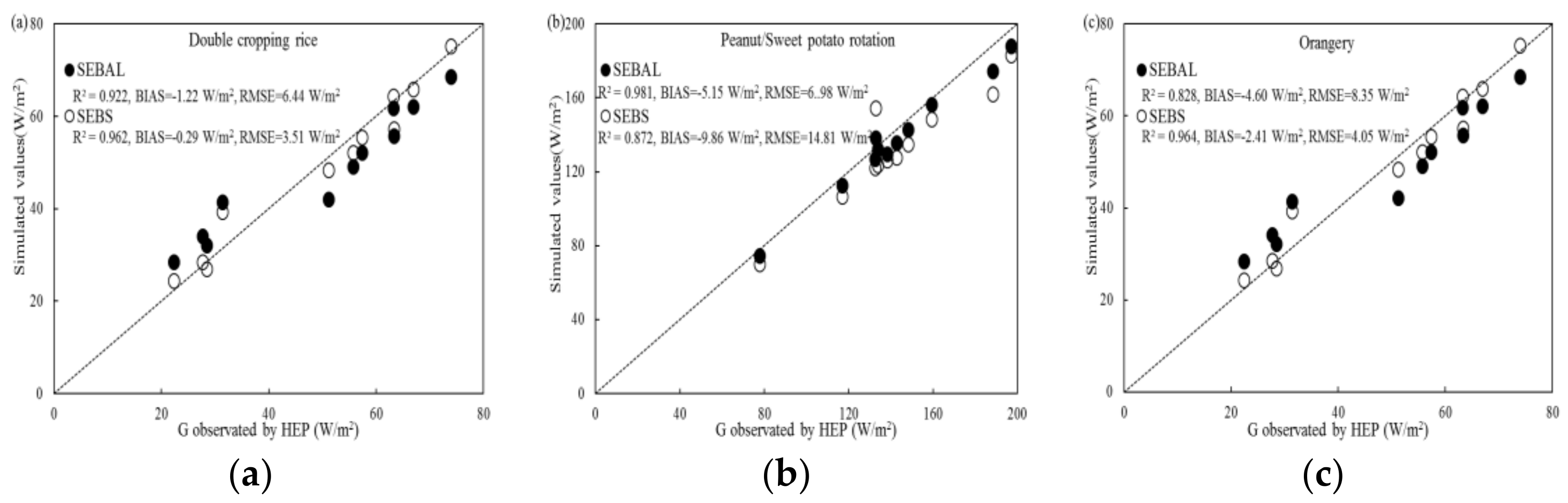
Then, the instantaneous results of the two models with the observed values from three soil heat flux plates on three different crop types were compared (Figure 3). The R², BIAS, and RMSE of the simulation results of SEBAL in the paddy field were 0.922, −1.22 W/m² and 6.44 W/m², respectively, while in SEBS, they were 0.962, −0.29 W/m² and 3.51 W/m², respectively. The R², BIAS, and RMSE of the simulation results of SEBAL in day farmland were 0.981, −5.15 W/m² and 6.98 W/m², respectively, while in SEBS, they were 0.872, −9.86 W/m² and 14.81 W/m², respectively. the R², BIAS, and RMSE of the simulation results of SEBAL in the orange grove were 0.828, −4.60 W/m² and 8.35 W/m², respectively, while in SEBS, they were 0.964, −2.41 W/m² and 4.05 W/m², respectively. Thus, the simulation results of SEBS in the paddy field and orange grove were closer to the observed values than the results using SEBAL (Figure 3a,c). However, the soil heat flux simulated by SEBAL in dry farmland was closer to the observed value (Figure 3b). The comparative results show that the SEBS model is relatively better in areas with high vegetation coverage (paddy field and orange grove), meanwhile SEBAL is better in areas with lower vegetation coverage (dry farmland).

4.2. Validation of Sensible Heat Flux

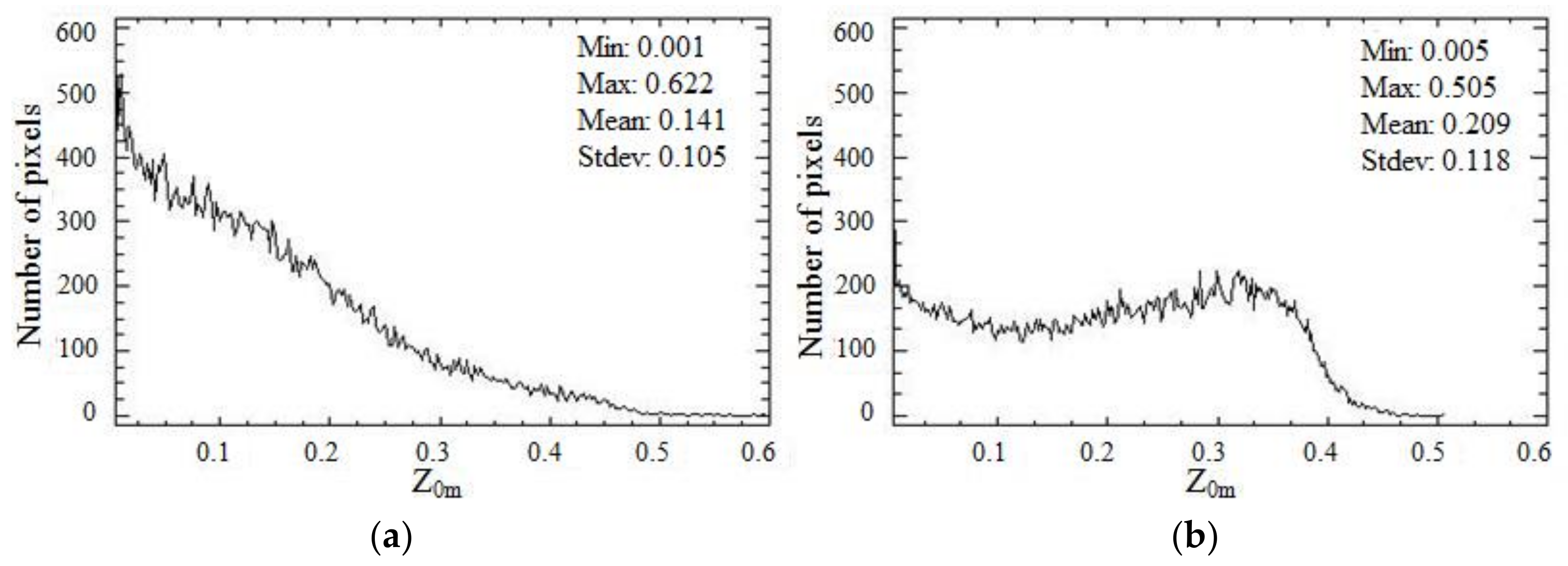
When considering the influence of geomorphic topographic relief over heterogeneous terrain, the surface kinetic parameters used in surface ET research are mainly the roughness length for momentum, z_om, and the zero plane displacement, d₀. As described before, the methods for the surface kinetic parameters are different between SEBAL and SEBS, which led to a significant difference in the distribution of roughness for momentum between SEBAL and SEBS (Figure 4). The number of pixels from the minimum z_om to the maximum z_om decreased progressively in SEBAL. However, in SEBS, the basic distribution pattern of the number of pixels from the minimum z_om to 0.36 showed very little dispersion, but once z_om became greater than 0.36, the number of pixels plummeted.

The sensible heat flux is determined by the temperature gradient between the surface and the atmosphere. The two models used different kinetic parameter calculation methods to estimate H, and they also differed in the selection of atmospheric stability correction methods. This could lead to differences between their sensible heat flux estimates. However, the overall trends for sensible heat flux estimated by the two models were roughly the same (Figure 5). H in dry farmland was larger than for other crop types. This trend is consistent with previous research [51,52]. At the ecosystem scale, the errors between the regional average simulated by the models and the observed value from LAS are mainly caused by the heterogeneity of the surface [53].

4.3. Validation of Daily ET

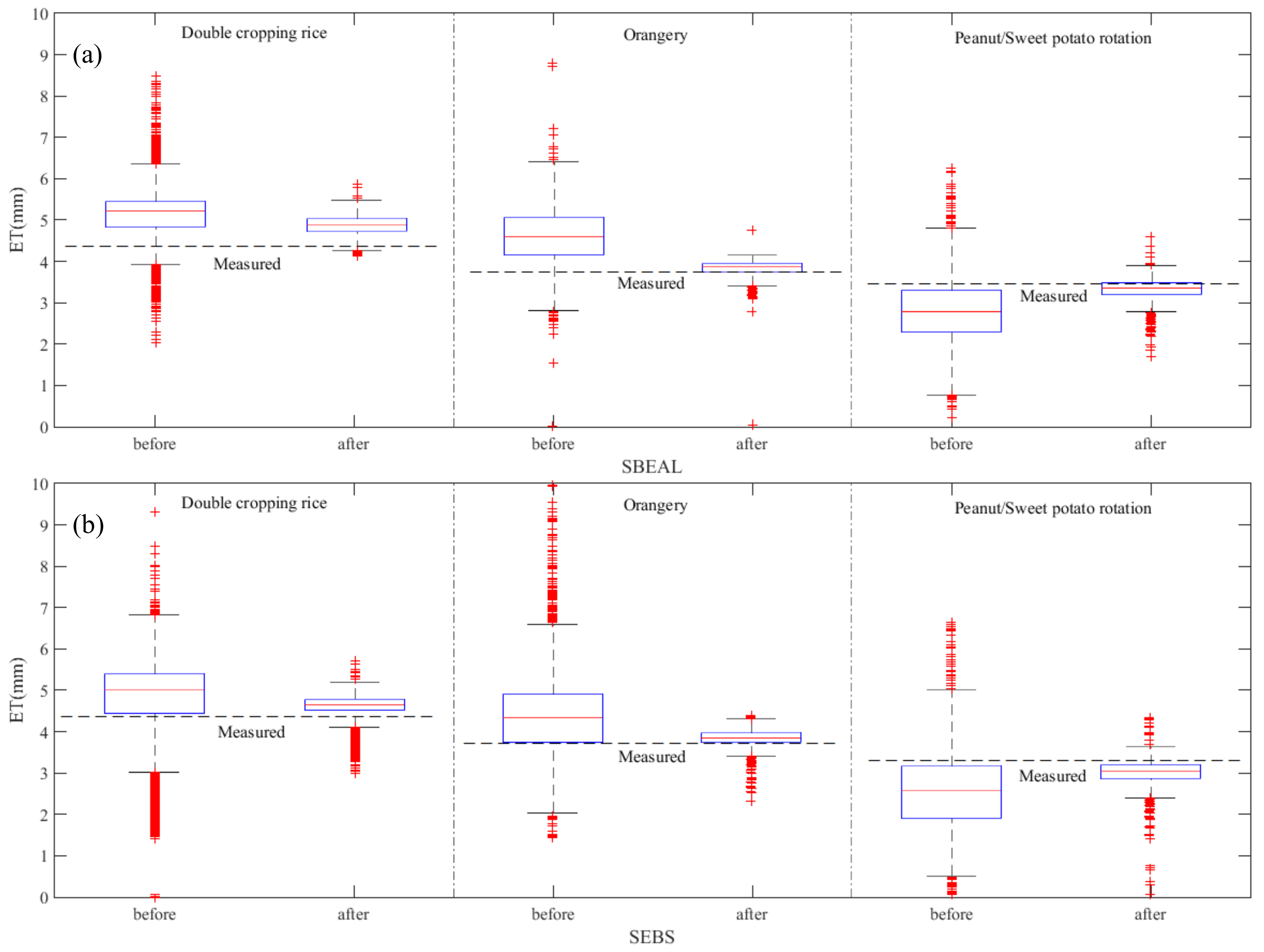
The measured values based on the Bowen/AWS and LAS were used to validate the ET simulated by the two single-source models at both site pixel and ecosystem scales. The results are shown in Figure 6. In SEBAL, the daily ET of each pixel ranged from 0.6 mm to 10.9 mm, the average daily ETs from the paddy field, dry farmland and orange grove were 5.157 mm, 2.861 mm and 4.349 mm, respectively. In SEBS, the daily ET of each pixel ranged from 0.9 mm to 11.5 mm, and the average daily ETs for the paddy field, dry farmland and grove were 4.973 mm, 2.363 mm and 4.212 mm (Figure 6), respectively.

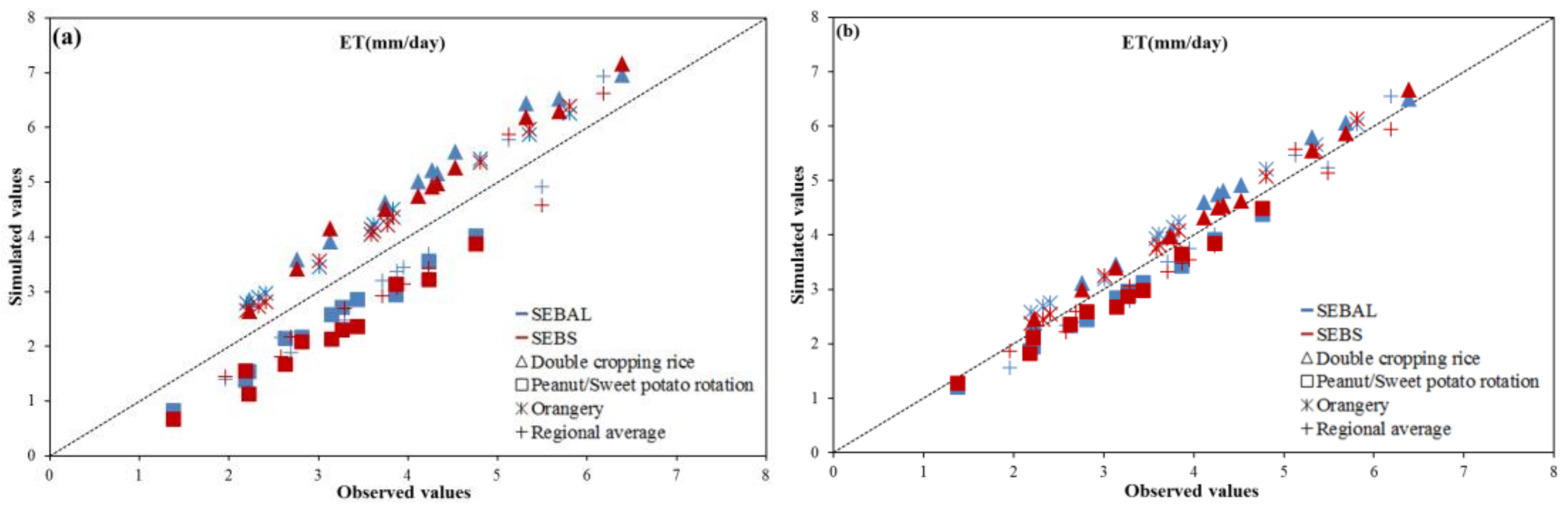
Based on the comparison with the results of the LAS footprint model, the mean absolute percent difference (MAPD) of the regional average daily ET in SEBAL was 15.27%, whereas, in SEBS, the MAPD of the regional average daily ET was 26.07% (Figure 6). The relative precision at the site scale for double-cropped rice, peanut/sweet potato rotation, and orange groves was 119.04%, 83.22%, and 115.08% in SEBAL and 114.80%, 68.73%, and 111.46% in SEBS, respectively. At the ecosystem scale, the relative precision of SEBAL and SEBS weas 86.75% and 79.32%, respectively (Figure 7a).

According to the above validation results, both the SEBAL and SEBS models tended to overestimate actual observations in the paddy field and orange grove pixels but tended to underestimate actual observations in dry farmland (Figure 6 and Figure 7a). Site investigations and the land-cover classification shown in Figure 1a,b revealed that vegetation pixels at a spatial resolution of 30 m exhibited surface heterogeneity due to the influence of planting factors. Therefore, this study assumed that the errors in the results were due to the mixed-pixel problem, which resulted in a substantial decrease in the simulation accuracy of the models and appeared to be the cause of over- and underestimates of various phenomena.

4.4. LSMM Improvements

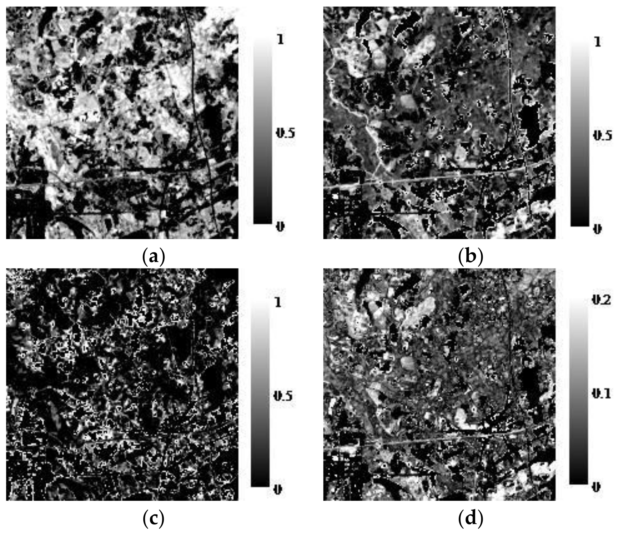
Surface heterogeneity caused by mixed pixels has a significant impact on model simulation. Errors in water and heat flux estimation caused by mixed pixels cannot be neglected. Thus, the LSMM was introduced to minimize errors caused by mixed pixels and to improve the estimation accuracy of the model. First, the mixed pixels in remote-sensing images were decomposed, and abundance values and root mean square errors (RMSE) were obtained for the three land-cover types. The results are shown in Figure 8. The RMSE statistics show that despite the RMSE maximum value of 0.2, approximately 90% of the pixels had RMSE values ranging from 0 to 0.06. The accuracy of linear spectral unmixing meets the requirements.

Then, the abundances of the three kinds of end-member were used as inputs for Equation (27). The ET contribution rates of the three kinds of land-cover type (rice, peanuts, and orange groves) to each mixed pixel were produced. Finally, these contribution rates were used to revise the SEBAL and SEBS simulation results. The pre-improved data simulated by SEBAL and SEBS were more discrete in all kinds of land cover types (Figure 6 and Figure 7a), while the improved results were more significantly concentrated (Figure 6 and Figure 7b). Figure 6 shows both the pre-improved (before) and improved (after) results from SEBAL and SEBS. The ET estimates for paddy fields, dry farmland, and orange groves by SEBAL and SEBS were both significantly improved by applying LSMM. The regional average ET values after applying LSMM were also closer to the measured values. The relative precision of ET estimated by the two models, with and without application of LSMM are given in

Table 2. Statistics of SEBAL and SEBS estimated versus observed ET at single point and ecosystem scales (MAD: mean absolute difference; MAPD: mean absolute percent difference; RMSE: root mean squared error).

Model			Double Cropping Rice	Peanut/Sweet Potato Rotation	Orangery	Regional Average
SEBAL	Relative Precision	Pre-improved	119.04%	83.22%	115.08%	86.75%
		Improved	110.99%	90.98%	109.53%	94.62%
	MAD	Pre-improved	0.834	0.577	0.57	0.524
		Improved	0.476	0.31	0.36	0.213
	MAPD	Pre-improved	16.17%	20.16%	13.11%	15.27%
		Improved	9.90%	9.91%	8.70%	5.70%
	RMSE (mm/day)	Pre-improved	0.86	0.67	0.55	0.62
		Improved	0.37	0.32	0.34	0.31
SEBS	Relative Precision	Pre-improved	114.80%	68.73%	111.46%	79.32%
		Improved	104.73%	86.56%	104.05%	89.38%
	MAD	Pre-improved	0.641	0.687	0.433	0.818
		Improved	0.205	0.462	0.153	0.42
	MAPD	Pre-improved	12.89%	29.07%	10.28%	26.07%
		Improved	4.52%	15.52%	3.89%	11.88%
	RMSE (mm/day)	Pre-improved	0.71	0.91	0.49	0.72
		Improved	0.22	0.32	0.20	0.34

. The relative precision at a site scale for double-cropped rice, peanut/sweet potato rotation, and orange groves were improved by 8.05%, 7.76%, and 5.55% in SEBAL, and 10.07%, 17.83%, and 7.41% in SEBS, respectively. The RMSE at a site scale for double-cropped rice, peanut/sweet potato rotation, and orange groves were improved by 0.49 mm/day, 0.35 mm/day, and 0.21 mm/day in SEBAL, and 0.49 mm/day, 0.59 mm/day, and 0.29 mm/day in SEBS, respectively. At a, ecosystem scale, the mean absolute percent differences (MAPD) of the improved regional average daily ET in both SEBAL and SEBS were much smaller than those for pre-improved conditions. The relative precision of SEBAL and SEBS was improved by 7.87% and 10.06%, respectively. The RMSEs of SEBAL and SEBS were improved by 0.31 mm/day and 0.38 mm/day, respectively. Although the total area of double-cropped rice in the study area was larger than that of peanuts, the area abundance of peanuts was more significant than that of rice in the observation area of the instrument (Figure 8). The orangery area was small, and the distribution was more dispersed. Thus, while both single-source models overestimated rice and orangery ET estimates, the overall relative precision of the regional average ET compared to the LAS observations was low (Table 2).

5. Summary and Conclusions

This study examined ET in a typical small, hilly, agricultural watershed in Yingtan City, Jiangxi Province, China. This agricultural watershed is an agroforestry system including paddy fields, dry farmland, and orange groves. Landsat8 satellite data with a spatial resolution of 30 m were used to invert various energy components and daily ET values for the study area. The differences in various energy components and parameters were investigated by SEBAL and SEBS simulations for three vegetation types (paddy fields, dry farmland, and orange groves). Bowen/AWS and LAS observational data were used to verify ET estimates of the two kinds of single-source energy balance models. This study also introduced the LSMM approach to unmix the images to reduce ET errors due to mixed pixels caused by surface heterogeneity and to improve model estimation accuracy.

The two models were validated at single point and ecosystem scales. The results of the two models showed that paddy field and orange grove pixels were overestimated to varying degrees, whereas dry farmland pixels were underestimated.

The land-cover classification (Figure 1) showed that vegetation pixels at a spatial resolution of 30 m exhibit surface heterogeneity due to the influence of planting factors. Therefore, LSMM was used to unmix the image of the study area and to obtain the abundance of paddy fields, dry farmland, and orange grove in each pixel. The results of the ET simulations with SEBAL and SEBS were then revised by incorporating the flux contribution rate of each end-member, as calculated by the least-squares method according to the overdetermined equations. The revised results show that the problem of over- and underestimation in various pixels in the two models was better solved.

There have been few available Landsat8 clear-sky images for the study area in recent years, and there are discontinuities in the remote-sensing data available for use. Therefore, this study could not improve model precision over time. The authors intend to expand the scope of the research in follow-up studies by developing an improved mixed-pixel decomposition model at multiple sites in China in different seasons and different growth periods. These studies will explore the impact of different time scales on the model and further improve the equations. It is anticipated that LSMM can be used to solve the problem of heterogeneity error at flux sites around the world.

References

- Allen, R.G.; Pruitt, W.O.; Businger, J.A.; Fritschen, L.J.; Jensen, M.E.; Quinn, F.H. Evaporation and Transpiration, in Hydrology Handbook, 2nd ed.; Heggen, R.J., Wootton, T.P., Cecilio, C.B., Fowler, L.C., Hui, S.L., Eds.; American Society of Civil Engineers: New York, NY, USA, 1996; pp. 125–252. [Google Scholar]
- Seguin, B.; Itier, B. Using midday surface temperature to estimate daily evaporation from satellite thermal IR data. Int. J. Remote Sens. 1983, 4, 371–383. [Google Scholar] [CrossRef]
- Kustas, W.P.; Daughtry, C.S.T.; Van Oevelen, P.J. Analytical treatment of the relationships between soil heat flux/net radiation ratio and vegetation indices. Remote Sens. Environ. 1993, 46, 319–330. [Google Scholar] [CrossRef]
- Carlson, T.N.; Capehart, W.J.; Gillies, R.R. A New Look at the Simplified Method for Remote Sensing of Daily ET. Remote Sens. Environ. 1995, 54, 161–167. [Google Scholar] [CrossRef]
- Menenti, M.; Choudhury, B. Parameterization of Land Surface Evaporation by Means of Location Dependent Potential Evaporation and Surface Temperature range; IAHS Publications: Oxfordshire, UK, 1993; pp. 561–568. [Google Scholar]
- Bastiaanssen, W.G.M. Regionalization of Surface Flux Densities and Moisture Indicators in Composite Terrain. Ph.D. Thesis, Wageningen Agricultural University, Wageningen, The Netherlands, 1995. [Google Scholar]
- Bastiaanssen, W.G.M.; Menenti, M.; Feddes, R.A.; Holtslag, A.A.M. A remote sensing surface energy balance algorithm for land (SEBAL): 1. Formulation. J. Hydrol. 1998, 212–213, 198–212. [Google Scholar] [CrossRef]
- Bastiaanssen, W.G.M.; Pelgrum, H.; Wang, J.; Ma, Y.; Moreno, J.F.; Roerink, G.J.; Van der Wal, T. A remote sensing surface energy balance algorithm for land (SEBAL): 2. Validation. J. Hydrol. 1998, 212–213, 213–229. [Google Scholar] [CrossRef]
- Bastiaanssen, W.G.M. SEBAL-based sensible and latent heat fluxes in the irrigated Gediz Basin, Turkey. J. Hydrol. 2000, 229, 87–100. [Google Scholar] [CrossRef]
- Su, Z. The surface energy balance system (SEBS) for estimation of turbulent heat fluexes. Hydrol. Earth Syst. Sci. 2002, 6, 85–99. [Google Scholar] [CrossRef]
- Roerink, G.J.; Su, Z.; Menenti, M. A Simple Remote Sensing Algorithm to Estimate the Surface Energy Balance. Phys. Chem. Earth. 2000, 25, 147–157. [Google Scholar] [CrossRef]
- Allen, R.G.; Tasumi, M.; Trezza, R. Satellite-based energy balance for mapping ET with internalized calibration (METRIC)-model. J. Irrig. Drain. Eng. 2007, 133, 380–394. [Google Scholar] [CrossRef]
- Shuttleworth, W.J.; Gurney, R.J. The Theoretical Relationship between Foliage Temperature and Canopy Resistance in Sparse Crop. Q. J. R. Meteorol. Soc. 1990, 116, 497–519. [Google Scholar] [CrossRef]
- Norman, J.M.; Kustas, W.P.; Humes, K.S. A Two-source Approach for Estimating Soil and Vegetation Energy Fluxes from Observation of Directional Radiometric Surface Temperature. Agric. For. Meteorol. 1995, 77, 263–293. [Google Scholar] [CrossRef]
- Anderson, M.C.; Norman, J.M.; Diak, G.R.; Kustas, W.P.; Mecikalski, J.R. A two-source time-integrated model for estimating surface fluxes using thermal infrared remote sensing. Remote Sens. Environ. 1997, 60, 195–216. [Google Scholar] [CrossRef]
- Kite, G.W.; Droogers, P. Comparing ET estimates from satellites, hydrological models and field data. J. Hydrol. 2000, 229, 3–18. [Google Scholar] [CrossRef]
- Jia, L.; Su, Z.; van den Hurk, B.; Menenti, M.; Moene, A.; De Bruin, H.A.R.; Javier, J.; Yrisarry, B.; Ibanez, M.; Antonio, C. Estimation of sensible heat flux using the surface energy balance system (SEBS) and ATSR measurements. Phys. Chem. Earth. 2003, 28, 75–88. [Google Scholar] [CrossRef]
- Timmermans, W.J.; Kustas, W.P.; Anderson, M.C.; French, A.N. An intercomparison of the Surface Energy Balance Algorithm for Land (SEBAL) and the Two-Source Energy Balance (TSEB) modeling schemes. Remote Sens. Environ. 2007, 108, 369–384. [Google Scholar] [CrossRef]
- Teixeira, A.H.; Bastiaanssen, W.G.M.; Ahmad, M.D.; Bos, M.G. Reviewing SEBAL input parameters for assessing ET and water productivity for the Low-Middle San Francisco River basin, Brazil Part A: Calibration and validation. Agric. For. Meteorol. 2009, 149, 462–476. [Google Scholar] [CrossRef] [Green Version]
- Ning, J.; Gao, Z.Q.; Xu, F.X. Effects of land cover change on evapotranspiration in the Yellow River Delta analyzed with the SEBAL model. J. Appl. Remote Sens. 2017, 11, 016009. [Google Scholar] [CrossRef]
- Vinukollu, R.K.; Wood, E.F.; Ferguson, C.R.; Fisher, J.B. Global estimates of evapotranspiration for climate studies using multi-sensor remote sensing data: Evaluation of three process-based approaches. Remote Sens. Environ. 2011, 115, 801–823. [Google Scholar] [CrossRef]
- Chen, X.; Su, Z.; Ma, Y.; Yang, K. Estimation of surface energy fluxes under complex terrain of Mt. Qomolangma over the Tibetan Plateau. Hydrol. Earth Syst. Sci. 2013, 17, 1607–1618. [Google Scholar] [CrossRef]
- Tang, R.; Li, Z.L.; Jia, Y.; Li, C.; Sun, X.; Kustas, W.P.; Anderson, M.C. An intercomparison of three remote sensing-based energy balance models using Large Aperture Scintillometer measurements over a wheat–corn production region. Remote Sens. Environ. 2011, 115, 3187–3202. [Google Scholar] [CrossRef]
- Sharma, V.; Kilic, A.; Irmak, S. Impact of scale/resolution on evapotranspiration from landsat and modis images. Water Resour. Res. 2016, 52, 1207–1221. [Google Scholar] [CrossRef]
- Byun, K.; Liaqat, U.W.; Choi, M. Dual-model approaches for evapotranspiration analyses over homo- and heterogeneous land surface conditions. Agric. For. Meteorol. 2014, 197, 169–187. [Google Scholar] [CrossRef]
- Rouholahnejad Freund, E.; Fan, Y.; Kirchner, J.W. Averaging over spatial heterogeneity leads to overestimation of ET in large scale Earth system models. In Proceedings of the EGU General Assembly Conference, Vienna, Austria, 23–28 April 2017; Volume 19. [Google Scholar]
- Ershadi, A.; McCabe, M.F.; Evans, J.P.; Chaney, N.W.; Wood, E.F. Multi-site evaluation of terrestrial evaporation models using FLUXNET date. Agric. For. Meteorol. 2014, 187, 46–61. [Google Scholar] [CrossRef]
- Gibson, L.A.; Münch, Z.; Engelbrecht, J. Particular uncertainties encountered in using a pre-packaged SEBS model to derive evapotranspiration in a heterogeneous study area in South Africa. Hydrol. Earth Syst. Sci. 2011, 15, 295–310. [Google Scholar] [CrossRef] [Green Version]
- Mcaneney, K.G.; Green, A.E.; Astill, M.S. Large Aperture Scintillometry: The Homogeneous Case. Agric. For. Meteorol. 1995, 76, 149–162. [Google Scholar] [CrossRef]
- Meijninger, W.M.L.; Hartogensis, O.K.; Kohsiek, W.; Hoedjes, J.C.B.; Zuurbier, R.M.; De Bruin, H.A.R. Determination of area-averaged sensible heat fluxes with a large aperture scintillometer over a heterogeneous surface–Flevoland field experiment. Bound.-Layer Meteorol. 2002, 105, 37–62. [Google Scholar] [CrossRef]
- Su, Z.; Schmugge, T.; Kusta, W.P.; Massman, W.J. An evaluation of two models for estimation of the roughness height for heat transfer between the land surface and the atmosphere. J. Appl. Meteorol. 2001, 40, 1933–1951. [Google Scholar] [CrossRef]
- Brutsaert, W. Aspects of Bulk Atmospheric Boundary Layer Similarity under Free-Convective Conditions. Rev. Geophys. 1999, 37, 439–451. [Google Scholar] [CrossRef]
- Monin, A.S.; Obukhov, A.M. Basic laws of turbulent mixing in the surface layer of the atmosphere. Tr. Akad. Nauk SSSR Geophiz. Inst. 1954, 24, 1963–1987. [Google Scholar]
- Monteith, J.L. Principles of Environmental Physics; Edward Arnold Press: London, UK, 1973; 241p. [Google Scholar]
- Massman, W.J. A model study of kB-1 for vegetated surfaces using “localized near-field” Lagrangian theory. J. Hydrol. 1999, 223, 27–43. [Google Scholar] [CrossRef]
- Timmermans, J.; Su, Z.; van der Tol, C.; Verhoef, A.; Verhoef, W. Quantifying the uncertainty in estimates of surface–atmosphere fluxes through joint evaluation of the SEBS and SCOPE models. Hydrol. Earth Syst. Sci. 2013, 17, 1561–1573. [Google Scholar] [CrossRef]
- Van der Kwast, J.; Timmermans, W.; Gieske, A.; Su, Z.; Olioso, A.; Jia, L.; Elbers, J.; Karssenberg, D.; de Jong, S. Evaluation of the Surface Energy Balance System (SEBS) applied to ASTER imagery with flux-measurements at the SPARC 2004 site (Barrax Spain). Hydrol. Earth Syst. Sci. 2009, 13, 1337–1347. [Google Scholar] [CrossRef]
- Harman, I. The role of roughness sublayer dynamics within surface exchange schemes. Bound.-Layer Meteorol. 2012, 142, 1–20. [Google Scholar] [CrossRef]
- Tang, R.; Li, Z.L. Evaluation of two end-member-based models for regional landsurface evapotranspiration estimation from MODIS data. Agric. For. Meteorol. 2015, 202, 69–82. [Google Scholar] [CrossRef]
- Tang, R.; Li, Z.L.; Chen, K.S.; Jia, Y.; Li, C.; Sun, X. Spatial-scale effect on the SEBAL model for ET estimation using remote sensing data. Agric. For. Meteorol. 2013, 174–175, 28–42. [Google Scholar] [CrossRef]
- Lu, D.; Moran, E.; Batistella, M. Linear mixture model applied to amazonian vegetation classification. Remote Sens. Environ. 2015, 87, 456–469. [Google Scholar] [CrossRef] [Green Version]
- Roberto, D.S.J.; Lacruz, M.; Keil, M.; Kramer, J.M.C. A linear spectral mixture model to estimate forest and savanna biomass at transition areas in Amazonia. In Proceedings of the IEEE International Geoscience and Remote Sensing Symposium IGARSS, Hamburg, Germany, 28 June–2 July 1999; Volume 2, pp. 753–755. [Google Scholar]
- Musa, S.D.; Onwuka, S.U.; Eneche, P.S.U. Geospatial Analysis of Land Use/Cover Dynamics in Awka Metropolis, Nigeria: A Sub-pixel Approach. J. Geo-Environ. Earth Syst. Int. 2017, 11, 1–19. [Google Scholar] [CrossRef]
- Onwuka, S.U.; Eneche, P.S.U.; Ismail, N.A. Geospatial modeling and prediction of land use/cover dynamics in onitsha metropolis, nigeria: A sub-pixel approach. Br. J. Appl. Sci. Technol. 2017, 22, 1–18. [Google Scholar] [CrossRef]
- Hu, B.; Miller, J.R.; Chen, J.M.; Hollinger, A. Retrieval of the canopy leaf area index in the boreas flux tower sites using linear spectral mixture analysis. Remote Sens. Environ. 2004, 89, 176–188. [Google Scholar] [CrossRef]
- Weng, Q.H.; Hu, X.F.; Liu, H. Estimating impervious surfaces using linear spectral mixture analysis with multitemporal aster images. Int. J. Remote Sens. 2009, 30, 4807–4830. [Google Scholar] [CrossRef]
- Zhang, Y.; Li, L.; Chen, L.; Liao, Z.; Wang, Y.; Wang, B.; Yang, X. A modified multi-source parallel model for estimating urban surface evapotranspiration based on aster thermal infrared data. Remote Sens. 2017, 9, 1029. [Google Scholar] [CrossRef]
- Somers, B.; Asner, G.P.; Tits, L.; Coppin, P. Endmember variability in Spectral Mixture Analysis: A review. Remote Sens. Environ. 2011, 115, 1603–1616. [Google Scholar] [CrossRef]
- Shimabukuro, Y.E.; Smith, J.A. The least-squares mixing models to generate fraction images derived from remote-sensing multispectral data. IEEE Trans. Geosci. Remote Sens. 1991, 29, 16–20. [Google Scholar] [CrossRef]
- Inmanbamber, N.G.; Mcglinchey, M.G. Crop coefficients and water-use estimates for sugarcane based on long-term bowen ratio energy balance measurements. Field Crops Res. 2003, 83, 125–138. [Google Scholar] [CrossRef]
- Cain, J.D.; Ptw, R.; Meijninger, W.; Harde, B. Spatially averaged sensible heat fluxes measured over barley. Agric. For. Meteorol. 2001, 107, 307–322. [Google Scholar] [CrossRef]
- Evans, J.G.; Mcneil, D.D.; Finch, J.W.; Murray, T.; Harding, R.J.; Ward, H.C.; Verhorf, A. Determination of turbulent heat fluxes using a large aperture scintillometer over undulating mixed agricultural terrain. Agric. For. Meteorol. 2012, 166–167, 221–233. [Google Scholar] [CrossRef]
- Ezzahar, J.; Chehbouni, A.; Hoedjes, J.; Ramier, D.; Boulain, N.; Boubkraoui, S.; Cappelaere, B.; Descroix, L.; Mougenot, B.; Timouk, F. Combining scintillometer measurements and an aggregation scheme to estimate area-averaged latent heat flux during the amma experiment. J. Hydrol. 2009, 375, 217–226. [Google Scholar] [CrossRef]
Figure 1.
Map of the land cover types and instrument locations. (a) Land cover type (30 m resolution form Landsat8); (b) Land Cover Type (0.5 m resolution form Pleiades); (c) The large aperture scintillometer (LAS) source areas (90% flux contribution) and instrument locations, identical to the areas in the black boxes on (a,b).
Figure 2.
The distribution of soil heat flux (a) Surface Energy Balance Algorithm for Land (SEBAL), (b) Surface Energy Balance System (SEBS).
Figure 3.
Comparison of simulated soil heat flux with the observed values by soil heat flux plates: (a) double cropping rice, (b) peanut/sweet potato rotation, (c) orangery.
Figure 4.
Number of pixels statistics of roughness length for momentum (Z0m) (a) SEBAL, (b) SEBS.
Figure 5.
(a–c) Comparison of simulated sensible heat flux with the observed values by Bowen at a single point: (a) double cropping rice; (b) peanut/sweet potato rotation; (c) orangery; (d) Comparison of the simulated sensible heat flux with the observed values from LAS at the ecosystem scale.
Figure 6.
The evapotranspiration (ET) value contrast before and after improvement: (a) SEBAL, (b) SEBS.
Figure 7.
Comparison of simulated ET with the observed values: (a) The result of the original model; (b) the improved simulation results.
Figure 8.
Abundance distribution of three crop types and the RMSE of mixed pixel decomposition. (a) The abundance in each pixel in double cropping rice; (b) the abundance in each pixel in peanut/sweet potatoes; (c) the abundance in each pixel in orange groves; (d) the RMSE of mixed pixel decomposition.