Probability Analysis of the Water Table and Driving Factors Using a Multidimensional Copula Function

Abstract

The relationship between the water table and driving factors is a reliable theoretical reference for the reasonable planning of surface water resources and the water table. Previous research has neglected the distribution and probabilities of the water table. However, this paper analyzes the relationship between the water table and driving factors from a statistical perspective by correcting the variables and introducing the Kernel Distribution Estimation and the Copula Function. The average data of the buried depth of the phreatic water, annual irrigation volume of the surface water, and precipitation in the Jinghui Irrigation District in China from 1977 to 2013 were adopted. We precisely obtained the two-dimensional (2D) and three-dimensional (3D) Joint Distribution Function of each driving factor and the marginal distribution of the water table, calculate the conditional probability in different ranges, and exactly predict the design value of surface water irrigation giving set conditions. Eventually, we emphasize the importance of probability analysis and prediction in groundwater planning.

1. Introduction

The fluctuation and the consequent prediction of the water table is one of the key problems of hydrological environment management [1]. Reliable prediction methods of the water table play significant roles in terms of groundwater planning and comprehensive management [2]. Over the years, scholars have applied different methods to study the water table, including the Linear Regression Method [3,4], Clustering Method [5], ARIMA Model [6], Genetic Programming Method, Neutral Network Method [7], Wavelet Approach [8], and SVM (Support Vector Machine) method [9], as well as the joint application of several methods [10,11].

These research methods have helped scholars to define the fluctuation of the water table as well as to predict it. However, most of these methods conduct a point prediction instead of finding the probability of an occurrence in ranges, neglecting the specific distribution of variables.

The Copula Function can be viewed as a multivariate probability distribution with uniform marginal in the interval [0,1]. In 2003, the first application of the Copula Function in the field of hydrology was undertaken [12]. In recent years, it has been widely applied to various aspects of hydrological studies [13]. The main applications of the Copula Function include the analysis of: precipitation characteristics [12], the correlation between flood peak and flood volume [14,15], the frequency and recurrence interval of floods [16,17,18], characteristics of storms [19,20], the frequency and recurrence intervals of droughts [21], drought assessment [22], risk assessment [23], and an assessment of environmental hydrological model performance [24]. Due to the specialty of the water table, the establishment of the Copula Function for this purpose is relatively difficult; therefore, no research that uses the Copula Function to analyze the water table has been reported. When considering the flexibility of the Copula Function establishment, this paper proposes that the Copula Function can be used to analyze the relationship between groundwater and driving factors from the perspective of probability.

The Jinghui Irrigation District, formerly known as Zhengguoqu in ancient times, is one of the four water resource projects in China. Its groundwater recharge mainly comes from surface water irrigation and precipitation. The method of surface water irrigation that was adopted in the Jinghui Irrigation District is flooding irrigation. Wheat in this area is irrigated three times a year in times of normal runoff, one time in winter, and two times in spring. In the case of low or high runoff, the irrigation frequency of the wheat can be adjusted as needed. Winter irrigation is conducted around the middle ten days of December. Spring irrigation is divided into three stages: the jointing stage, heading stage, and the filling stage. In terms of the irrigation volume, the fixed irrigation volume of winter irrigation is 9 × 10⁴ m³/km² to 10.5 × 10⁴ m³/km², and that of the spring irrigation is 6 × 10⁴ m³/km² to 7.5 × 10⁴ m³/km². The total annual irrigation volume is less than 18 × 10⁴ m³/km² to 22.5 × 10⁴ m³/km². Corn in this area is irrigated one to two times in wetter years, and three to four times in dry years. The irrigation period is from July to September, and the fixed irrigation volume is 6 × 10⁴ m³/km² to 7.5 × 10⁴ m³/km². The total annual irrigation volume of the corn is less than 19.5 × 10⁴ m³/km² to 27 × 10⁴ m³/km². However, the actual irrigation varies according to the different situations each year. Recharging from the irrigation water infiltration is the major source of replenishment of the groundwater. Research data has indicated that, in the 1980s, the water irrigation infiltration volume utilized at least 30% of the surface water diversion; in the 1990s, the percentage dropped to about 25%; and, from 1997 to 2009, it dropped to less than 20%. After 2010, the percentage began to slowly increase again. In addition to surface water diversion, precipitation infiltration is another way to recharge groundwater. However, the effects of the latter are obviously smaller than those of the former [25]. The Jinghui Irrigation District plays an important role in Chinese national economic life. Therefore, it has frequently been the target of research. However, this research has mainly focused on qualitative analysis and water quality. Research on the water table of the Jinghui Irrigation District is relatively rare, but it includes the research by Liu Y. (2010), who analyzed the dynamic transformation of the groundwater of the Jinghui Irrigation District from 1977 to 2005 using the Multivariate Linear Regression Method [4]. This indicated that, ceteris puribus, if the annual precipitation of the district varies by 10 mm, the buried depth of the groundwater will vary by 3.5 cm approximately; similarly, for every million m³ of surface water irrigation volume in the district, the average buried depth of the groundwater varies 2.4 cm consequently, and for every million m³ of groundwater mining, the average buried water table in the Jinghui Irrigation District varies by ±0.53 mm. Obviously, when compared with the amount of groundwater mining, the irrigation volume of the surface water and precipitation are two significant factors that affect the buried depth of the phreatic water. Additionally, due to the data collection method, the data regarding of the amount of groundwater mining is not stable enough. Given the same conditions, the more groundwater mining that there is, the smaller the buried depth of the groundwater is, which is contrary to what occurs in reality. Although the amount of groundwater mining is a relatively important factor that affects the buried depth of the phreatic water, unstable data may lead to incorrect conclusions. Therefore, given the fixed conditions of the present amount of groundwater mining (140 ± 4 million m³), this paper analyzes the relatively stable data of the buried depth of the phreatic water, the annual irrigation volume of the surface water, and the precipitation through the Copula Function from a statistical perspective.

In order to make explicit the probabilistic relations between the water table and the driving factors, so that these can be used to offer more reliable references for the planning and management of water resources, this paper mainly focuses on the following: (1) Estimating the marginal distribution function of each driving factor through the Kernel distribution method. (2) Establishing the two-dimensional (2D) Copula Function of each driving factor and the marginal distribution of the water table through the 2D Copula Function, and analyzing the response of each driving factor to the buried depth of groundwater. The 2D Copula Function can be built directly, and its fitting results are satisfactory. (3) Since the buried depth of the phreatic water is negatively correlated with the annual precipitation and annual irrigation volume of the surface water, the fitting results of the three-dimensional (3D) Copula Function—which is directly built through the 3D Symmetric Archimedean Copula Function—are not satisfactory. Therefore, in undertaking a real application, this paper corrects the variables first, which consequently leads to an acceptable fitting result. Again, the 3D Copula Function is applied to comprehensively analyze the response of the irrigation volume of the surface water and the annual precipitation to the buried the depth of the phreatic water when the two factors, respectively, vary. In addition, the results are compared with those of the 2D Copula Function. (4) This paper also calculates the conditional probability values. Given fixed conditions, we calculate the probability of the water table falling into different ranges, together with the volume of surface water irrigation that should lead to the expected water table.

2. Materials and Methods

2.1. Study Area and Data

2.1.1. Introduction of the Irrigation Area

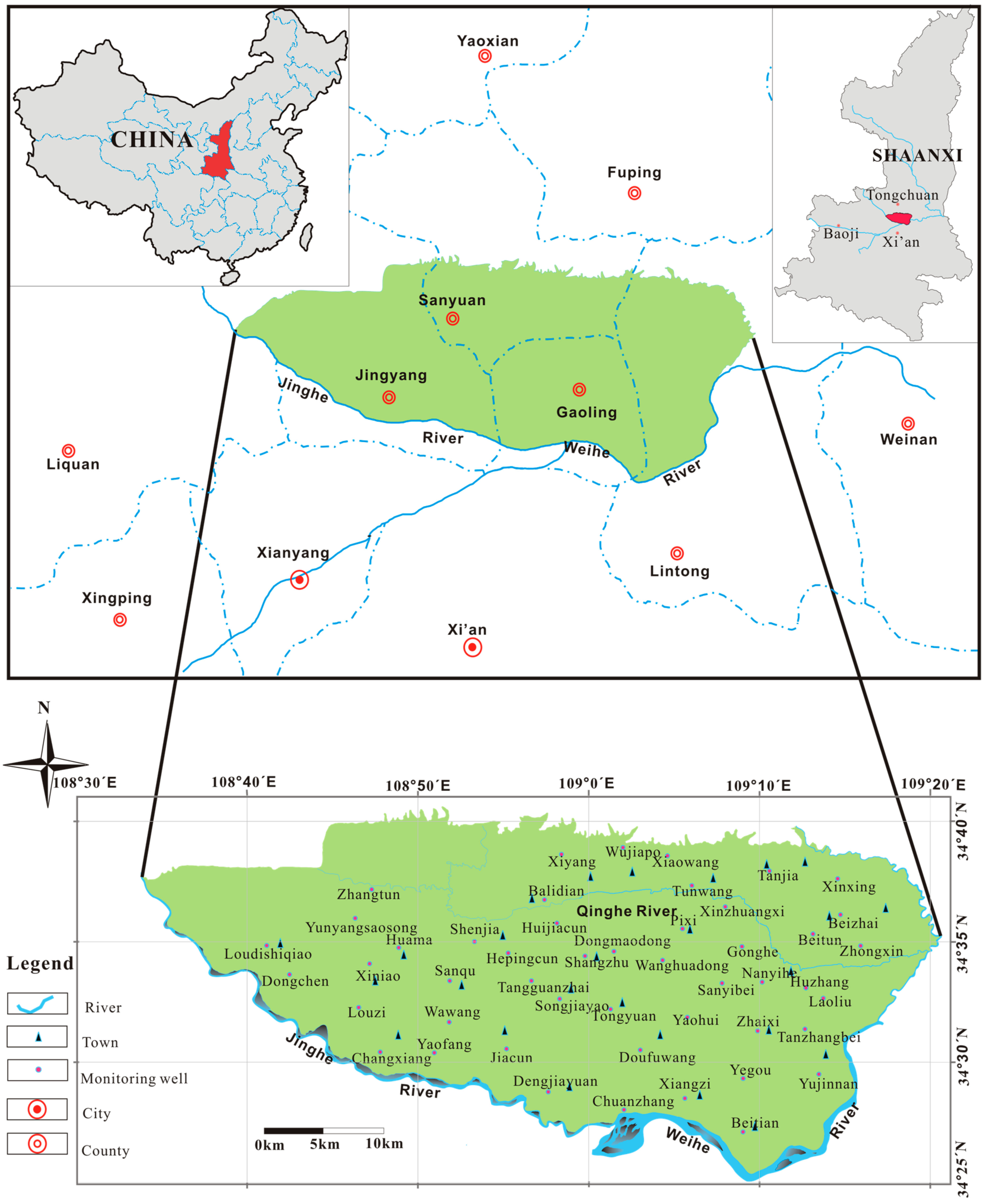
The Jinghui Irrigation District is a gravity irrigation project that draws water from the Zhongshan Mountain Pass, Jinghe River, Jingyang County, Shaanxi Province. It is located in the center of the Guanzhong Plain, 34°25′20″ to 34°41′40″ N, 108°34′34″ to 109°21′35″ E (see Figure 1). To the east of the irrigation district lies the Shichuan River; to the west, the Jinghe River; to the south, the Weihe River; and, to the north, the Weibei Loess Platform. The elevation of the district is between 350 m and 450 m. The district is located in the continental semi-arid climate zone; therefore, high temperatures and concentrated precipitation occur in summer. Almost 60% of the annual precipitation happens from June to September. However, in the winter, it is cold and dry, and there is less precipitation. The annual evaporation capacity is approximately 1212 mm. The average temperature of the district is 13.6 °C; the maximum air temperature ever recorded was 42 °C (1996), and the lowest air temperature that has been recorded was −24 °C (1955). The length of the irrigation district from east to west is approximately 70 km, the width from south to north is approximately 20 km, the total area of the district is about 1180 km², the designated irrigation area of the district is 9.7102 km², and the active area is 9102 km² [26]. Soil in the district is fertile and rich, and crops that are planted in the district include wheat, corn, cotton, and vegetables, with a multiple crop index that is greater than 1.85. All of these factors make the district one of the main grain-producing areas in the Shaanxi Province. Occupying 2.4% of the provincial farmland, the Jinghui Irrigation District once produced 5.7% of the grain in the Shaanxi Province [4]. The buried depth of the phreatic water in the district directly affects its agricultural production and hydrogeological environment, while the irrigation volume of the surface water and precipitation directly affect the buried depth of the phreatic water in the district. Therefore, it is necessary to study the relationships between them.

2.1.2. Data

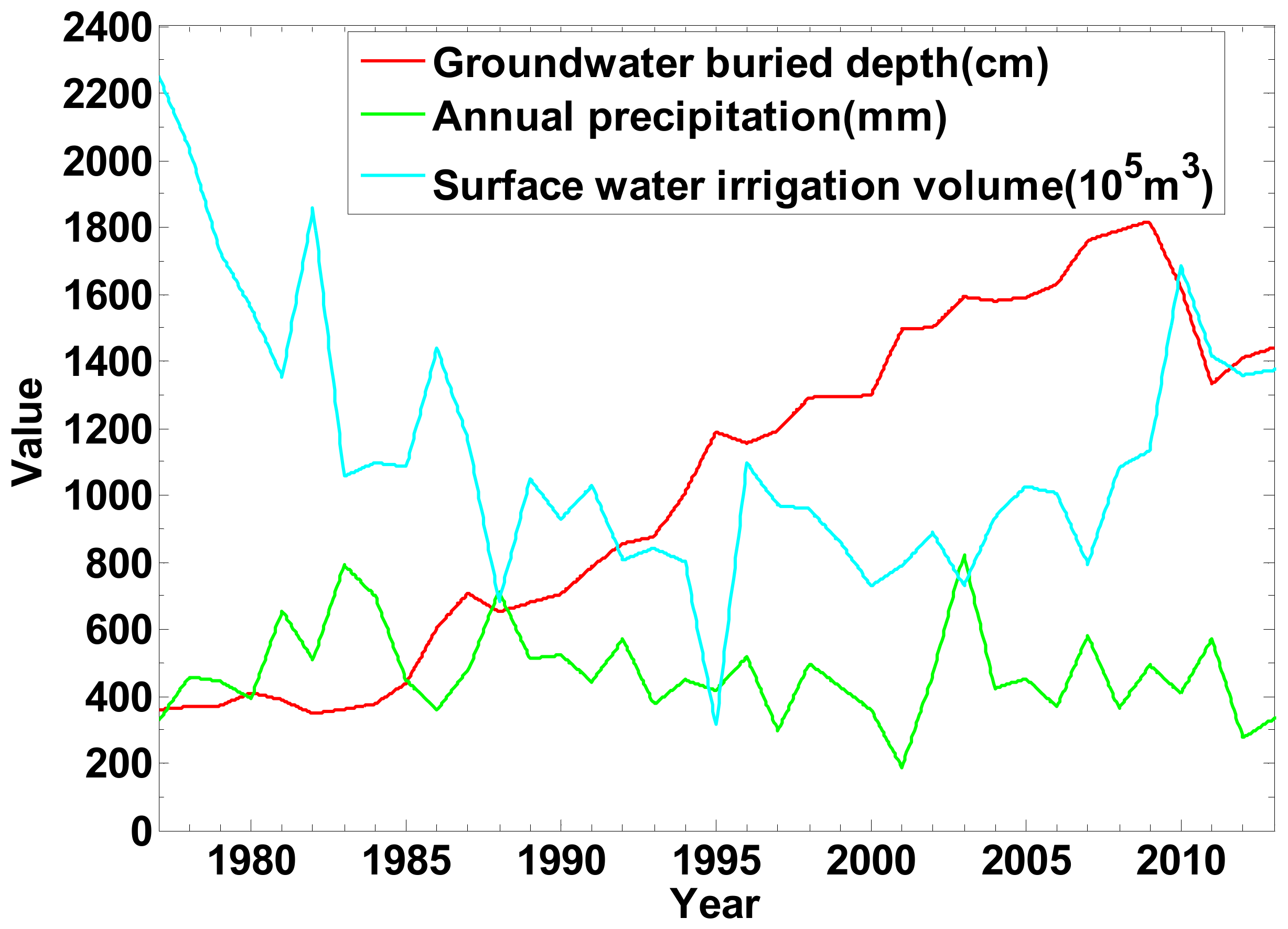
The data of the phreatic water buried depth used in the paper came from the monitoring data from January 1977 to December 2013 from 48 wells in the Jinghui Irrigation District. The frequency of monitoring for this dataset is once a month. We obtained the annual average water level of each well through calculating the arithmetic average of the monitoring data from January to December each year. Combining this with the control area of each well, we then computed the annual average water level of the district through a weighted average calculation. The locations of the wells are shown in Figure 1. For the data of the surface water irrigation volume, we adopted the annual total irrigation volume of the district. The data of the phreatic water buried depth and the surface water irrigation volume were taken from the monitoring and statistical data of the Shaanxi Jinghuiqu Administration. Due to the relatively small area of the district, there is only one monitoring point for annual precipitation. Therefore, the data of annual precipitation was obtained through the summation of precipitation data from January to December each year recorded by the monitoring point, which was obtained from the Shaanxi Provincial Meteorological Bureau. Figure 2 shows the development of the three variables over time.

2.2. Methodology

2.2.1. Theory of the Copula Function

Copula Function was first utilized by Sklar (1959) in the 1950s [27]. It can structure the multidimensional joint distribution function through a marginal distribution and correlation structure. The Copula function models the nonlinearity, symmetry, or asymmetry of the dependence structure of the variables [28]. Sklar’s theorem states that $X_1, X_2,\cdots , X_n$ are random variables, $F_1\left(x_1\right), F_2\left(x_2\right),\cdots ,F_n\left(x_n\right)$ are its marginal distribution function, F is the joint probability distribution function of the n-dimension, therefore, there must exist the Copula Function $\mathrm{C}{\left[0,1\right]}^n\to \left[0,1\right]$, which makes the following formula true:

$$F\left(x_1,x_2,\cdots ,x_n\right)=C\left[F_1\left(x_1\right),F_2\left(x_2\right),\cdots ,F_n\left(x_n\right)\right]$$

(1)

In the formula, C represents the Copula Function.

If the marginal distribution function $F_1\left(x_1\right),F_2\left(x_2\right),\cdots ,F_n\left(x_n\right)$ are continuous, then the Copula Function will be unique [27].

Commonly used 2D Copula Functions in the hydrological field include three Archimedean Copula Functions: Gumbel-Hougaard (GH), Clayton, and Frank, as shown in

Table 1. 2D Archimedean Copula Functions.

Copulas	CDF	Parameters
Gumbel-Hougaard	$\exp \{-{[(-\ln u){}^{\theta }+\left(-\ln v{)}^{\theta }\right)]}^{1/\theta \}}$ }	$\theta >0$
Clayton	${(u^{-\theta }+v^{-\theta }-1)}^{-1/\theta }$	$\theta \ge 1$
Frank	$-\frac{1}{\theta }\ln$ (1+ $\frac{\left(e^{-\theta u}-1\right)\left(e^{-\theta v}-1\right)}{e^{-\theta }-1}$ )	$\theta \ne 0$

Note: $\theta$ is the parameter of Copula Function.

[28,29].

The Archimedean Copula Model with two variables can effectively establish the joint distribution function of the buried depth of the groundwater and irrigation volume of the surface water, and the 2D joint distribution of the marginal distribution of the groundwater’s buried depth and the annual precipitation. However, there is more than one main driving factor that affects the groundwater buried depth. Due to the simple structure and the convenient application of the Symmetric Archimedean Copula Function with a single parameter, this paper adopts the typical 3D Symmetric Archimedean Copula Function to conduct further analysis.

The 3D Symmetric Archimedean Copula Function includes the Gumbel-Hougaard Copula, Clayton Copula, and Frank Copula, whose distribution functions are listed in

Table 2. Three-dimensional (3D) Symmetric Archimedean Copula Functions.

Copulas	CDF	Parameters
Gumbel-Hougaard	$\exp \{-{[(-\ln u_1){}^{\theta }+(-\ln u_2){}^{\theta }+(-\ln u_3){}^{\theta }]}^{1/\theta }\}$	$\theta \ge 1$
Clayton	${(u_1{}^{-\theta }+u_2{}^{-\theta }+u_3{}^{-\theta }-2)}^{-1/\theta }$	$\theta >0$
Frank	$-\frac{1}{\theta }\ln [\frac{\left(e^{-\theta u_1}-1\right)\left(e^{-\theta u_2}-1\right)\left(e^{-\theta u_3}-1\right)}{{(e^{-\theta }-1)}^2}]$	$\theta \ne 0$

[28,29,30,31].

2.2.2. Marginal Probability Distribution

The correctness of the marginal distribution directly affects the correctness of the joint distribution function. Commonly used methods that use samples to estimate the probability density function of the ensemble include the parametric estimation method and the non-parametric estimation method. The parametric estimation method requires the ensemble to be subjected to a certain known distribution, and then estimates the parameters through samples. However, some commonly used density functions are unable to reflect the probability distribution characteristics of actual data, thus making the results unsatisfactory.

This paper adopts the Kernel Density Estimation (KDE) method to estimate the probability density function of the ensemble [32].

If we assume that $X_1,X_2,\dots X_n$ are the samples of a one-dimension continuous ensemble $X$, then the Kernel Density of the probability density function $f\left(x\right)$ of $X$ is defined as:

$$\widehat{f_h}\left(x\right)=\frac{1}{nh}{\displaystyle \sum }_{i=1}^{n}K\left(\frac{x-X_i}{h}\right)$$

(2)

In this equation, h represents the bandwidth and K (·) represents the Kernel Function. Since the Kernel Density Estimation is insensitive to the selection of the Kernel Function, the Gaussian Kernel Function is adopted [33,34]:

$$K\left(x\right)=\frac{1}{\sqrt{2\pi }}\exp \left(-\frac{1}{2}{x}^2\right)$$

(3)

In the Kernel Density Estimation, the values of the bandwidth h will affect the smoothness of the Kernel Density Function $\widehat{f_h}\left(x\right)$; if the value of h is relatively large, then the image of $\widehat{f_h}\left(x\right)$ will be smoother, however, it will lose certain information that is contained in the data. On the contrary, if the value of h is relatively small, the image of $\widehat{f_h}\left(x\right)$ will be composed of rough break lines, but it can more accurately reflect the information that is contained in each data point. It can be concluded that the appropriate value of the bandwidth h is therefore of great importance. Thus, we adopt the method used by Shimazaki and Shinomoto based on the Mean Integrated Square Error (MISE) principle to obtain the optimum bandwidth [35]. The Kolmogorov-Smirnov goodness-of-fit test (K-S) (Yevjevich, 1972) is applied to check the Marginal Probability Distribution model [36].

K-S Test:

$H_0$: Assume the totality we took the sample from is subjected to a certain distribution.

$H_1$: Assume the totality we took the sample from is not subjected to a certain distribution.

The test statistic D of the K-S Test is expressed as follows:

$$D=\max \left\{\left|F_n\left(x\right)-F\left(x\right)\right|\right\}$$

(4)

In the above equation, $F_n\left(x\right)$ is the empirical distribution function and $F\left(x\right)$ is the theoretical distribution function.

If $D>d_{\partial }$, then the original assumption is rejected, otherwise it is accepted. $d_{\partial }$ is the critical value when the significance level is $\partial$, and $\partial$ is the significance level. The value of $d_{\partial }$ can be obtained using Monte Carlo techniques [37,38].

2.2.3. Estimation of Parameters and Model Checking of the Copula Function

The parameters of the 2D and 3D Copula Functions are estimated using the Maximum Likelihood Estimation Method [39]. The R Copula package was used for the goodness-of-fit test [40,41]. The Akaike Information Criterion (AIC) was used to select the Copula Function with the best fit [30,42].

AIC Method:

The formula of the AIC is expressed as follows:

$$\mathrm{AIC}=n\ln \left(\mathrm{MSE}\right)+2m$$

(5)

In this formula, MSE represents the mean square error, n represents the number of samples, and m is the number of independently adjusted parameters.

2.2.4. Conditional Distribution

For 2D variables, the marginal distributions of X and Y are, respectively [28,37]:

$$F_X\left(x\right)=P\left(X\le x\right)=u,{\mathrm{F}}_Y\left(y\right)=P\left(Y\le y\right)=v$$

(6)

The conditional probability of an event taking place is:

$$P\left(y_1<Y<y_2|x_1<X<x_2\right)=\frac{P\left(x_1<X<x_2，y_1<Y<y_2\right)}{P(x_1<X<x_2)}=\frac{C\left(u_2,v_2\right)-C\left(u_1,v_2\right)-C\left(u_2,v_1\right)+C\left(u_1,v_1\right)}{\left(u_2-u_1\right)}$$

(7)

In this equation C represents the Copula Function.

For 3D variables, the conditional probability of two equivalent events is:

$$P\left(Z<z|X=x,Y=y,\right)=\frac{\frac{{\partial }^{2}C\left(u_1,u_2,u_3\right)}{\partial u_1\partial u_2}}{\frac{{\partial }^{2}C\left(u_1,u_2\right)}{\partial u_1\partial u_2}}$$

(8)

3. Results and Discussion

3.1. The Establishment of the Marginal Distribution

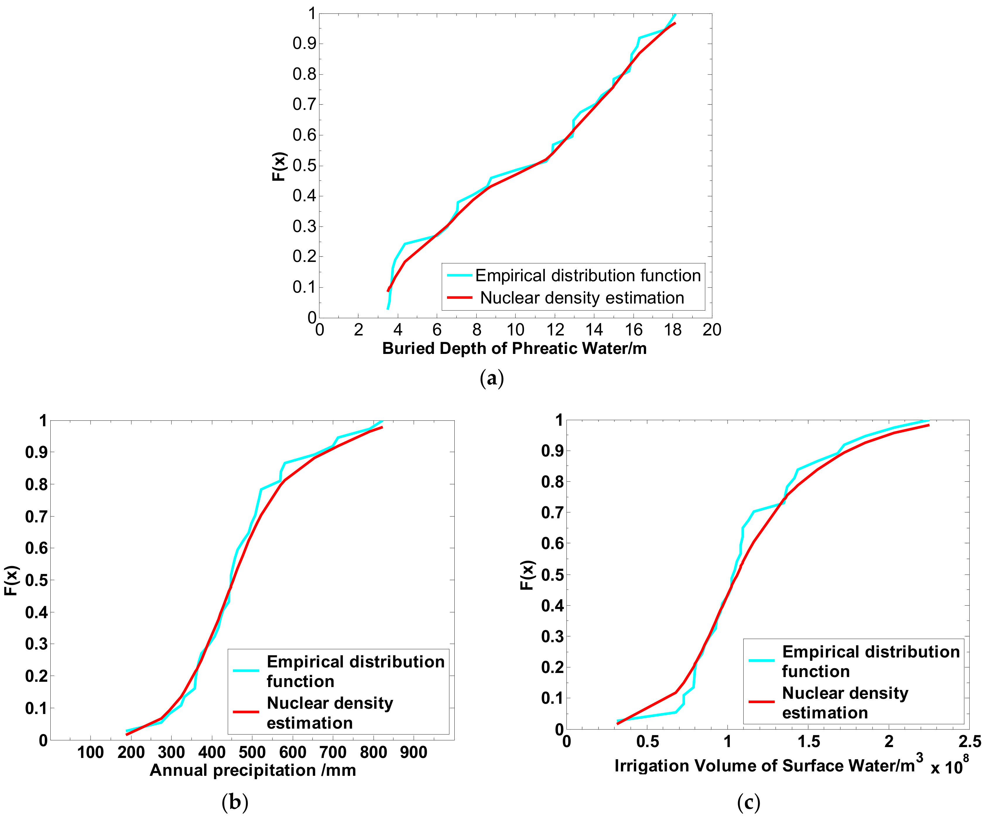
The marginal functions of the driving factors are estimated through the Kernel Distribution method. The fitting results are listed in

Table 3. Fitting results of marginal distribution functions.

Parameters	D1	P1	S1
D	0.0860	0.0804	0.1100
d0.05	0.1123	0.1257	0.1798

Note: D1 is the buried depth of the phreatic water (unit: m); P1 is the annual precipitation (unit: mm); S1 is the annual irrigation volume of the surface water (unit: 10⁸ m³); and, D is the statistic of the K-S checking test.

, and the images of the distribution functions are shown in Figure 3.

Referring to Table 3, all of the computed values of the test statistic D are lower than the critical values. It can therefore be concluded that all of the distribution functions that are estimated through the Kernel Distribution can undergo the tests. It can be inferred from Table 3 and Figure 3 that the Kernel Distribution Method can properly estimate the distribution functions of the driving factors.

3.2. Analysis of 2D Copula Function

3.2.1. The Establishment of 2D Joint Distribution Functions

Since the Gumbel and Clayton Copula can be used to describe the positive dependence between variables, the Frank Copula can therefore be used to describe the negative dependence between variables. The Kendall rank coefficients between pairs of variables were calculated and the Kendall independence test was undertaken. The results for the pairs of variables D1-S1, D1-P1, and P1-S1 were –0.28 (p-value: 0.013), –0.168 (p-value: 0.047) and 0.151 (p-value: 0.062), respectively. The Kendall rank coefficients pass the tau test at the 0.1 significance level. Therefore, combined with the marginal distribution demonstrated in Figure 3, we adopt the Frank Copula to fit the joint distribution function between the marginal distribution of the phreatic water buried depth and the marginal distribution of the surface water irrigation volume in the Jinghui Irrigation District. Then, the joint marginal distribution function fits between the marginal distribution of the phreatic water buried depth and the marginal distribution of the annual precipitation. The parameter of θ is estimated through the Maximum Likelihood Estimation Method. The R Copula package was used to test the goodness-of-fit. The values of the parameters and the model checking results are listed in

Table 4. Parameters of the Frank Copula Function and the fitting test results.

	θ	p-value	AIC
D1-S1	−3.0065	0.4856	−250.77
D1-P1	−1.9058	0.4254	−300.26

Note: The meanings of D1, S1 and P1 are the same as in Table 3.

.

It can be inferred from Table 4 that the Frank Copula Function could not be rejected at the selected significance level (0.05). Therefore, the Frank Copula is able to model the joint distribution function between marginal distributions.

Furthermore, it can be inferred from Table 1 and Table 4 that the joint distribution function of the marginal distribution of the groundwater buried depth and the annual irrigation volume of the surface water is as follows:

$$C_1\left(u_1，u_2\right)=\frac{1}{3.0065}\ln [1+\frac{\left(e^{3.0065u_1}-1\right)\left(e^{3.0065u_2}-1\right)}{(e^{3.0065}-1)}]$$

(9)

In this equation, $u_1=P\left(X\le x\right)$, $u_2=P\left(Y\le y\right)$, $X$ is the buried depth of the phreatic water, and $Y$ is the annual irrigation volume of the surface water.

The joint distribution function of the marginal distribution of the groundwater buried depth and annual precipitation in the Jinghui Irrigation District is as follows:

$$C_2\left(u_1，u_3\right)=\frac{1}{1.9058}\ln [1+\frac{\left(e^{1.9058u_1}-1\right)\left(e^{1.9058u_3}-1\right)}{(e^{1.9058}-1)}]$$

(10)

In the above equation, the meaning of $u_1$ is similar to in Equation (9), $u_3=P\left(Z\le z\right)$ and $Z$ is the annual precipitation.

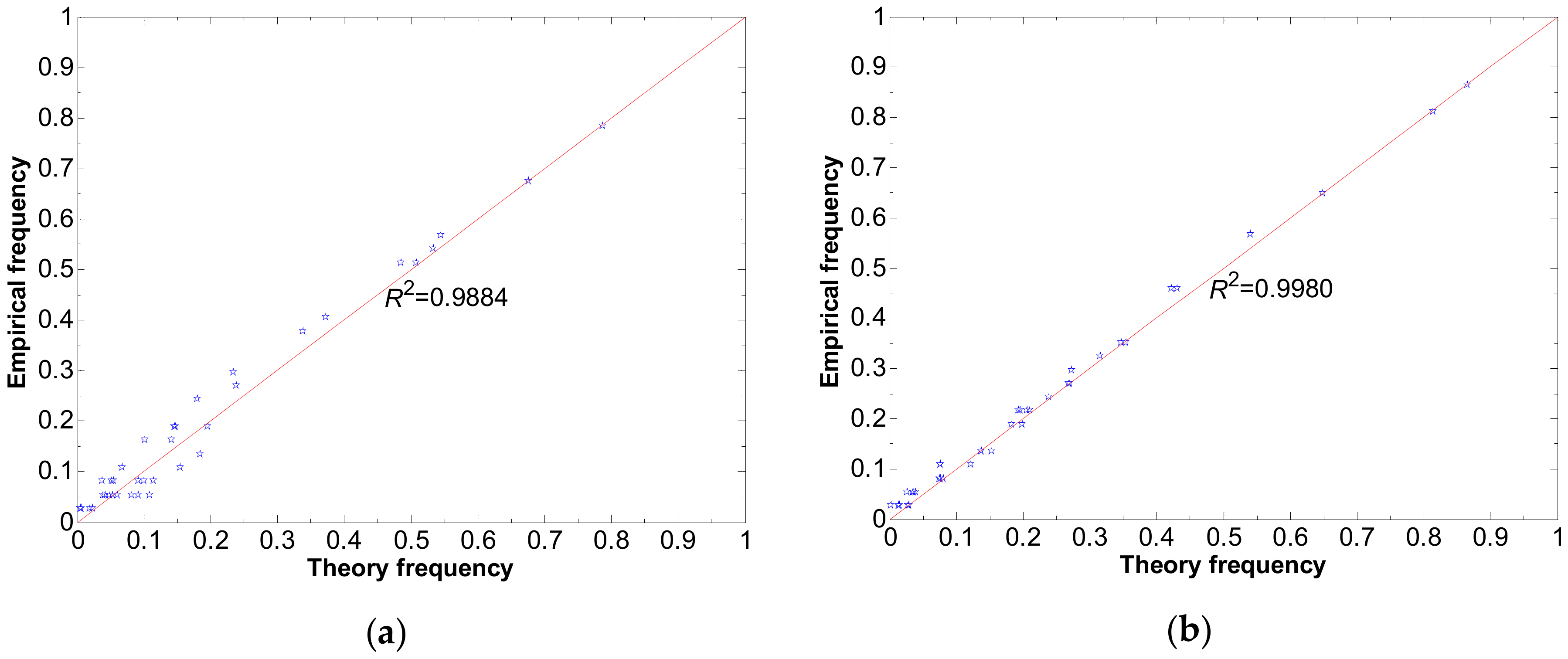
The correlation between the empirical frequency and theoretical frequency, and the image of the distribution function is shown in Figure 4.

The value of the correlation coefficient (R²) in Figure 4a,b is greater than 0.95. Therefore, when combining the results of Table 4 and Figure 4 we can conclude that the 2D Frank Copula Function can correctly describe the correlation between the buried depth of the phreatic water and the precipitation of Jinghuiqu and the correlation between the buried depth of the phreatic water and the irrigation volume of the surface water.

3.2.2. Calculation and Analysis of Conditional Probability

First, we divided the value variation into three ranges according to the data of the phreatic water buried depth, annual precipitation, and annual irrigation volume of the surface water over 37 years in the Jinghui Irrigation District. To prevent the effect of range length that is impacting on probability, the ranges are equally divided. Then, we adopt Equations (7), (9) and (10) to calculate the different conditional probability values. The results are listed in

Table 5. Conditional probability of buried depth falling into different ranges given the condition of the surface water irrigation volume in different ranges.

P(C1 < D1 < C2/C3 < S1 < C4)	0.31 < S1 < 0.96	0.96 < S1 < 1.61	1.61 < S1 < 2.25
3.60 < D1 < 8.46	0.1888	0.4538	0.6729
8.46 < D1 < 13.31	0.2653	0.2908	0.2103
13.31 < D1 < 18.17	0.5459	0.2554	0.1168

Note: C1, C2, C3, and C4 are random constants. The meanings of D1 and S1 are the same as in Table 3. P is the probability.

and

Table 6. Conditional probability of buried depth falling into different ranges given the condition of annual precipitation in different ranges.

P(C1 < D1 < C2/C3 < P1 < C4)	187.0 < P1 < 399.3	399.3 < P1 < 611.6	611.6 < P1 < 823.9
3.60 < D1 < 8.46	0.2377	0.4073	0.5659
8.46 < D1 < 13.31	0.2662	0.2809	0.2444
13.31 < D1 < 18.17	0.4961	0.3118	0.1897

Note: The meanings of D1 and P1 are the same as in Table 3; P, C1, C2, C3 and C4 are the same as in Table 5.

.

It can be inferred from Table 5 that, regardless of other factors, when the volume of the surface water irrigation falls into the maximum range (1.61 × 10⁸ m³ to 2.25 × 10⁸ m³), then the probability of the buried depth of the phreatic water falling into the minimum range (3.60 m to 8.46 m) reaches the maximum value (0.6729), which indicates that the lager the irrigation volume of the surface water, the bigger the probability of the phreatic water buried depth falling into the minimum range. Similarly, the smaller the irrigation volume of the surface water, the smaller the probability of the phreatic water buried depth falling into the minimum range of values.

Table 6 indicates that, regardless of other factors, when the annual precipitation falls into the maximum range (611.6 mm to 823.9 mm), the probability of the buried depth of the phreatic water falling into the minimum range (3.60 m to 8.46 m) reaches the maximum value (0.5659), which demonstrates that the larger the value for the annual precipitation, the greater the probability of the phreatic water buried depth falling into the minimum range of values. Similarly, the smaller the value for the annual precipitation, the smaller the probability of the phreatic water buried depth falling into the minimum range of values.

The aforementioned results agree with the results of previous qualitative analyses. The most important finding is the probability values of the buried depth of phreatic water falling into different value ranges when the precipitation and surface water diversion fall into different range values qualitatively, from the statistical perspective. Furthermore, we qualitatively validated the correlation between precipitation, surface water irrigation volume, and the buried depth of the phreatic water in the Jinghui Irrigation District.

3.3. 3D Copula Function Analysis

3.3.1. Establishment of the 3D Copula Function

The buried depth of the phreatic water is relevant to several factors in the Jinghui Irrigation District. Thus, the analysis of a single variable has limitations, for instance, being unable to reflect the mutual variation correlation between multiple factors. In order to predict the surface water diversion volume that is required by a certain probability given a certain level of precipitation in the district, we adopt a 3D Symmetric Archimedean Copula Function to fit the joint distribution functions of the marginal distribution of the buried depth of the phreatic water, annual irrigation volume of the surface water, and the annual precipitation in.

However, due to the negative correlation between the buried depth of the phreatic water and annual precipitation, and the buried depth of the phreatic water and the annual irrigation volume of the surface water, the commonly used 3D Symmetric Archimedean Copula Functions are unable to properly fit the joint distribution functions of buried depth, annual precipitation, and annual irrigation of the surface water. Therefore, we first corrected the buried depth variable. We chose a constant and subtracted the buried depth, calling this the relative elevation of water table, then fits the joint distribution functions of marginal distribution of the relative elevation of the water table, annual precipitation, and annual irrigation volume of the surface water. Such fitting results are satisfactory. Since the fitting result shares no correlation with the constant that is used while correcting the variable, its value can be zero for convenience. At this time, the relative elevation of the water table equals the negative buried depth of the phreatic water. However, Symmetric Copulas can be used in cases when the investigated variables are exchangeable. Therefore, a test of exchangeability that is provided by the R Copula package was carried out. Moreover, the test results for the pairs of variables ND1-S1, ND1-P1, and S1-P1 were 0.032 (p-value: 0.34), 0.026 (p-value: 0.52), and 0.028 (p-value: 0.48), respectively. This indicates that the Symmetric Copula Functions, which have one parameter to model the dependence among three variables, seems reasonable. The fitting results are listed in

Table 7. Different Archimedean Copula Function parameters and the fitting test results.

Parameters	Gumbel	Frank	Clayton
θ	1.1331	0.9889	0.2685
p-value	0.8632	0.7786	0.1816
AIC	−256.47	−258.98	−254.28

.

It can be inferred from Table 7 that the three Archimedean models could not be rejected at the selected significance level (0.05). Therefore, the three Copula Functions are all able to describe the correlations between variables. However, the AIC value of the Frank Function is the smallest, so we adopt the Frank Copula as the joint distribution function.

It can be seen from Table 2 and Table 7 that the joint distribution function of the marginal distribution of the negative buried depth of the phreatic water, annual irrigation volume of the surface water, and annual precipitation in the Jinghui Irrigation District is as follows:

$$C_3\left(u_1,u_2,u_3\right)=-\frac{1}{0.9889}\ln [1+\frac{\left(e^{-0.9889u_1}-1\right)\left(e^{-0.9889u_2}-1\right)(\left(e^{-0.9889u_3}-1\right)}{{(e^{-0.9889}-1)}^2}]$$

(11)

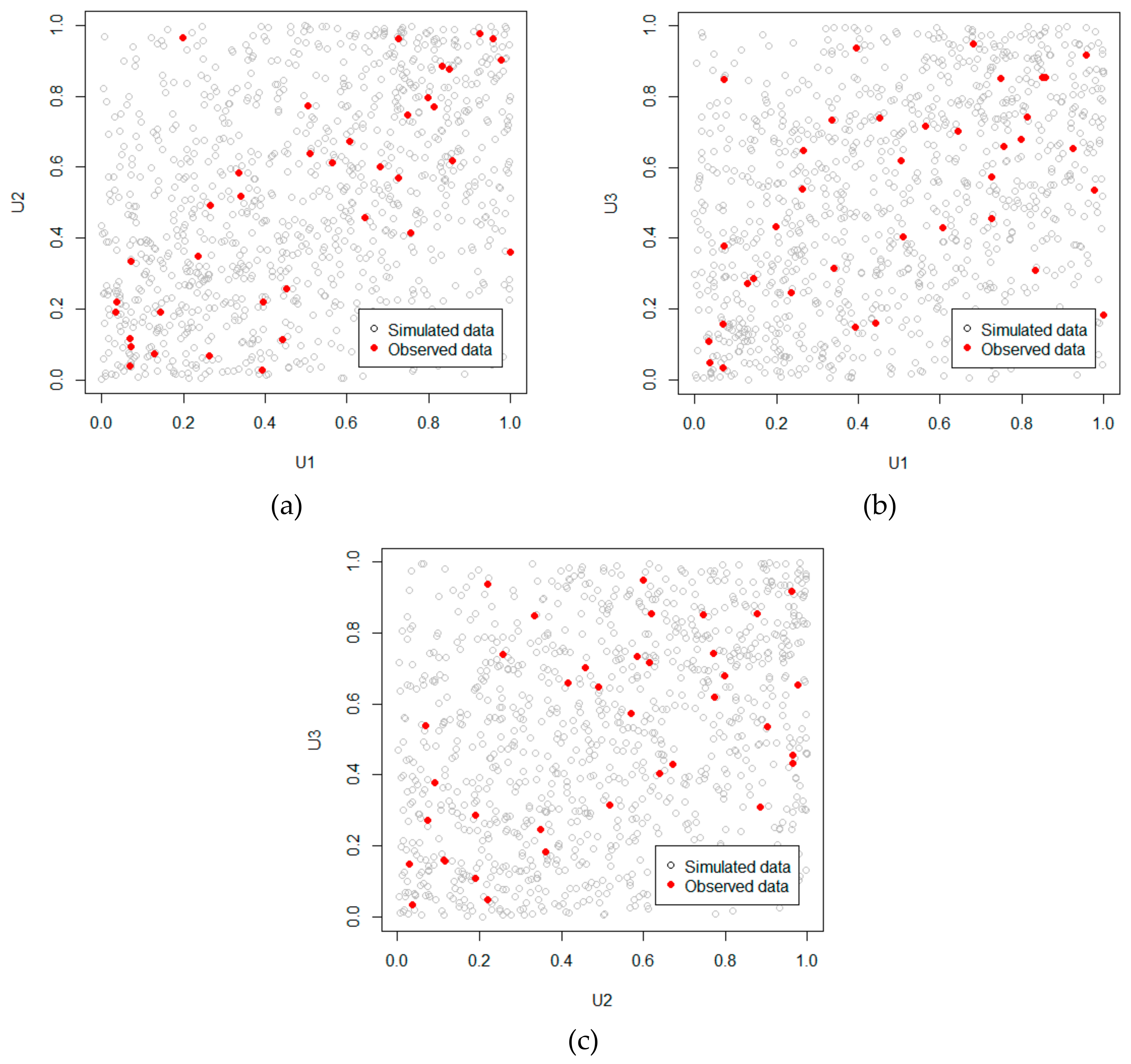
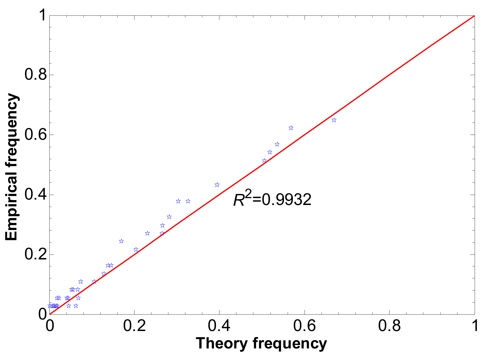
In the above equation, $u_1=P\left(X\le x\right)$, $u_2=P\left(Y\le y\right)$, $u_3=P\left(Z\le z\right)$, $X$ is the negative buried depth of the phreatic water, $Y$ is the annual irrigation volume of the surface water, and $Z$ is the annual precipitation. Plots of all the pairs of the simulated and observed data are shown in Figure 5. Q-Q (Quantile-Quantile) plots of the theoretical frequency and empirical frequency of the Frank Copula Function are shown in Figure 6.

When combining Table 7, Figure 5 and Figure 6, the 3D Symmetric Frank Copula Function can accurately describe the correlations among the negative buried depth of the phreatic water, annual surface water irrigation volume, and annual precipitation.

3.3.2. Calculation and Analysis of Conditional Probability

Similarly to the 2D Distribution Function, we also divide the reference historical data of the annual irrigation volume of the surface water and annual precipitation into three ranges, and calculate the probabilities of the groundwater buried depth falling into different ranges given that the irrigation volume of the surface water and precipitation fall into different ranges.

By comparing with the data shown in Table 6 and

Table 8. Probabilities of the groundwater buried depth falling into different ranges given that the irrigation volume of the surface water and precipitation fall into different ranges.

P(C1 < D1 < C2/C3 < S1 < C4,C6 < P1 < C5)		0.31 < S1 < 0.96	0.96 < S1 < 1.61	1.61 < S1 < 2.25
	3.60 < D1 < 8.46	0.2852	0.3151	0.3334
187.0 < P1 < 399.3	8.46 < D1 < 13.31	0.2674	0.2724	0.2743
	13.31 < D1 < 18.17	0.4474	0.4125	0.3923
	3.60 < D1 < 8.46	0.3206	0.4250	0.4925
399.3 < P1 < 611.6	8.46 < D1 < 13.31	0.2730	0.2748	0.2653
	13.31 < D1 < 18.17	0.4064	0.3002	0.2423
	3.60 < D1 < 8.46	0.3469	0.5066	0.6059
611.6 < P1 < 823.9	8.46 < D1 < 13.31	0.2750	0.2628	0.2351
	13.31 < D1 < 18.17	0.3781	0.2306	0.1590

Note: The meanings of D1, P1 and S1 are the same as in Table 3, P is the same as in Table 5.

, it can be inferred that, regardless of the irrigation volume of the surface water, given the condition that precipitation falls into the range of 187.0 mm to 399.3 mm, the conditional probability of the buried depth of the groundwater falling into the range of 3.60 m to 8.46 m is 23.77%. However, if taking the mutual effects of precipitation and irrigation volume of the surface water on the buried depth of the groundwater into consideration, then the first line in Table 8 indicates that at the same time that precipitation falls into the range of 187.0 mm to 399.3 mm, and the irrigation volume of the surface water falls into the range of 0.31 × 10⁸ m³ to 0.96 × 10⁸ m³, the conditional probability of the buried depth of the groundwater falling into the range of 3.60 m to 8.46 m becomes 28.52%, and the value continues to grow as the precipitation remains the same and the irrigation volume of the surface water grows. Table 6 also indicates that, regardless of the irrigation volume of the surface water, given the condition of precipitation being between 187.0 mm and 399.3 mm, the conditional probability of the buried depth of the groundwater falling into 13.31 m to 18.17 m (deeper) is 49.61%; however, if the mutual effects of precipitation and the irrigation volume of the surface water on the buried depth of the groundwater are considered simultaneously, the third line in Table 8 demonstrates that all of the calculated results are less than the value, while the probability value continues to decrease as the irrigation volume of the surface water increases. It is the negative correlation between the irrigation volume of the surface water and the buried depth of the groundwater that leads to such results.

Hence, it is obvious that the 2D Copula Function can reveal the relationship between the buried depth of the groundwater and each driving factor to some degree; however, the 3D Copula Function can take more driving factors into consideration simultaneously, which allows for it to reveal the mutual variation relationships between the buried depth of the groundwater and each driving factor in a more systematic and specific way.

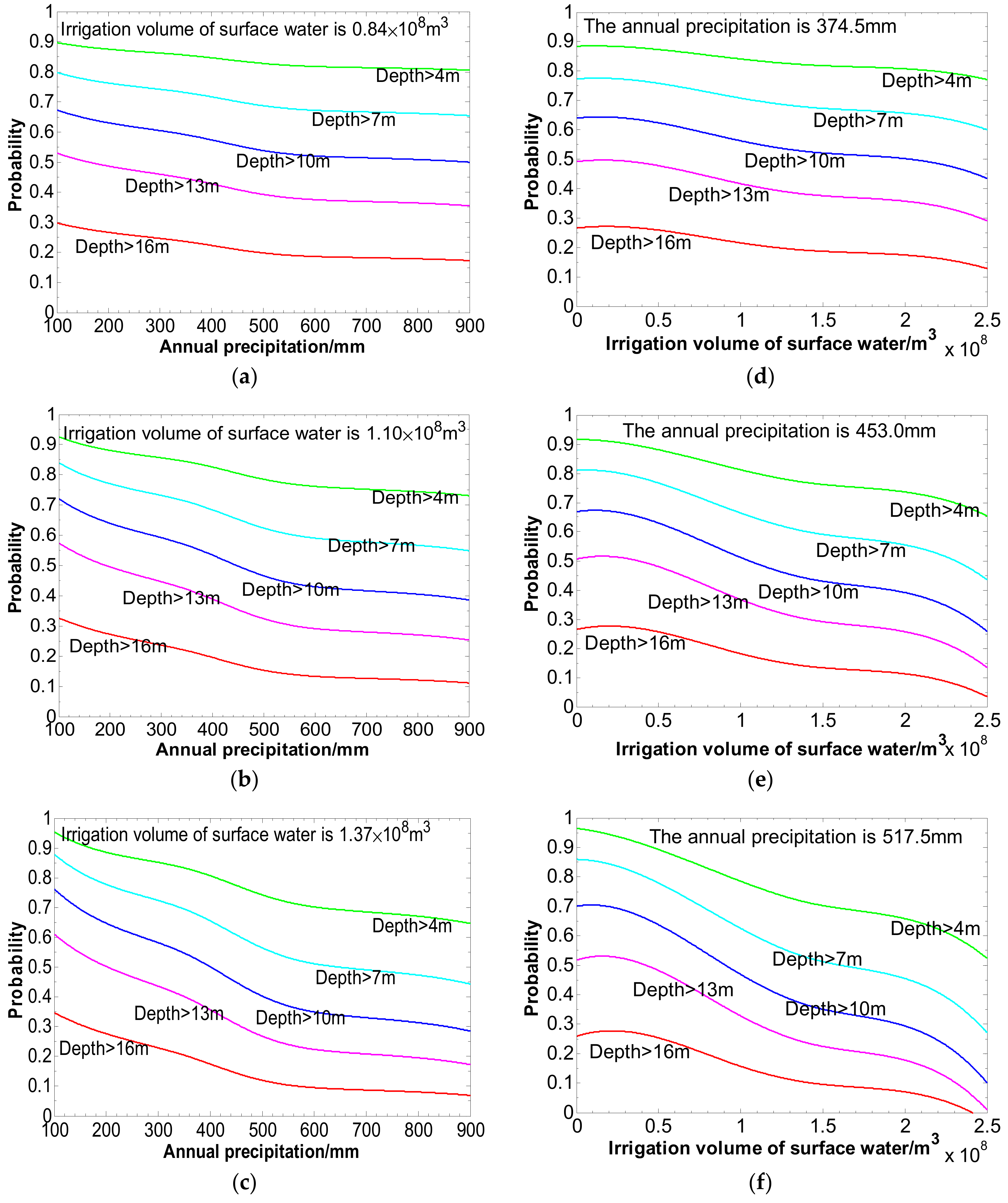
In practical applications, the buried depth of the groundwater under the condition of fixed precipitation and irrigation volume of the surface water requires further consideration. Therefore, we assigned the values of the surface water irrigation volume as low 0.84 × 10⁸ m³, normal 1.10 × 10⁸ m³, and high 1.37 × 10⁸ m³, and drew the conditional probability graph of the groundwater buried depth falling into different ranges given different precipitation levels, as seen in Figure 7a–c. Next, we assigned the precipitation levels as low 374.5 mm, normal 453.0 mm, and high 517.5 mm, and drew the conditional probability graph of the groundwater buried depth falling into different ranges given different irrigation volumes of the surface water, as Figure 7d–f indicate.

It can be inferred from Figure 7a–c that given a fixed irrigation volume of the surface water, the level of precipitation and the probability of the groundwater buried depth being greater than a certain value are negatively correlated; in other words, given a fixed irrigation volume of the surface water, the greater the value of the precipitation, the smaller the probability of the groundwater buried depth being greater than a certain value. The aforementioned result is in agreement with the conclusion of the 2D Copula Function. In addition, it is obvious that, as the surface water diversion grows, the slope of the curve increases as well, indicating that as the irrigation volume of the surface water grows, each growth of precipitation per unit will make the probability of the groundwater buried depth being greater than a certain value increase. Similarly, it can be inferred from Figure 7d–f, that given a fixed level of precipitation, the surface water diversion and the probability of the groundwater buried depth being greater than a certain value are negatively correlated. In other words, given a fixed level of precipitation, the larger the irrigation volume of surface water, the smaller the probability of the groundwater buried depth being greater than a certain value. Additionally, it is obvious that as the precipitation increases, the slope of the curve increases as well, indicating that as the precipitation level increases, each increase in the irrigation volume of the surface water per unit will make the probability of the groundwater buried depth being greater than a certain value increase. The results indicate that the level of precipitation and the irrigation volume of the surface water mutually promote this effect on the water table.

Figure 7 also showed the quantitative variation of the buried depth of the groundwater given the condition of typical precipitation and surface water diversion. In reality, more conditional probabilities can be calculated as needed with distribution functions, and the value calculated quantitatively is what we needed to regulate and control the water table. Figure 7a–c also indicates that regardless of high, low, or normal runoff of the surface water diversion, the probability that the buried depth of the groundwater greater than 16 m (deeper) decreases, the probability that the buried depth of the groundwater is smaller than 4 m increases, and the probability of the buried depth of the groundwater being between 4 m and 16 m remains relatively stable. Figure 7d–f also indicates that, regardless of high, low, or normal runoff of precipitation, as the irrigation volume of the surface water increases, the probability that the buried depth of the groundwater is greater than 16 m (deeper) is always decreasing, the probability that the buried depth of the groundwater is less than 4 m (shallower) is always increasing, and the probability that the buried depth of the groundwater is between 4 m and 16 m is unchanged.

Meanwhile, in practical applications, if the precipitation of a certain year needs to be predicted, the buried depth of the phreatic water can be controlled in the needed range through different irrigation volumes of the surface water. For instance, if the precipitation of a certain year is 453 mm and there is a 70% probability that the buried depth of the phreatic water will be less than 11 m, then the designated irrigation volume of the surface water should be no less than 1.70 × 10⁸ m³ (it is estimated that the average annual amount of water that can be diverted from Jinghuiqu is about 5.64 × 10⁸ m³ from 1977 to 2013, which has not changed much in recent years. Even if the rainfall in irrigation area is relatively low, sufficient water can be ensured for surface water irrigation.).

3.3.3. Discussion

Theoretically, a 3D Symmetric Copula Function with a single parameter can only describe the correlation between symmetric variables. In this paper, the correlations between parameters are not strictly in symmetry with each other, however, such a case is relatively common in practical applications. Although Asymmetric Copula functions with multiple parameters are able to describe the non-symmetric correlations between variables, this should never be adopted separately from the structure of asymmetric functions. If the asymmetric model departs form the actual correlation between variables, then the results will be unsatisfactory some of the time. Furthermore, the addition of unknown parameters will increase the difficulty of solving the model. It can be inferred from the model test results that are presented in this paper that a 3D Symmetric Frank Copula with a single parameter is already able to satisfactorily describe the correlations among the buried depth of the phreatic water, annual surface water irrigation volume and annual precipitation. Whether the fitting results of asymmetric models with multiple parameters are better is discussed in our following paper. The Archimedean Copula is not the only model that can describe the correlations among the buried depth of the phreatic water, annual surface water irrigation volume, and annual precipitation, however. The application of other Copula Functions still requires further study.

In terms of the actual situation of the Jinghui Irrigation District, although the influence of the amount of groundwater mining on the water level is less than the influence of the surface irrigation water volume, its role is greater than that of precipitation and other factors, therefore the amount of groundwater mining should also be a relatively important influencing factor on the water level. The more groundwater mining that occurs, the deeper the buried depth of the phreatic water. On the contrary, the less that groundwater mining occurs, the shallower the buried depth of the phreatic water. Therefore, if the amount of groundwater mining is increased in a certain year, if maintaining a shallower buried depth of the phreatic water within a certain range of probability is still required, then the actual diversion and the irrigation volume of the surface water should be correspondingly larger than the designated irrigation volume of the surface water calculated in this paper. We also suggest that the relevant departments can adjust the data collection method to collect more precise statistical data of the amount groundwater mining occurring, so that we can assess the water table of the Jinghui Irrigation District in more detail.

4. Conclusions

The paper introduces a 2D and 3D Frank Copula Function to analyze the responsiveness of different driving factors to the buried depth of the phreatic water. Consequently, the fitting results are satisfactory. Furthermore, the paper compared the results of the 3D Copula Function and 2D Copula Function, jointly analyzes the responsiveness of multiple varying driving factors on the buried depth of the phreatic water, and predicts the design volume of surface water irrigation given definite precipitation. This paper adopts data from the Jinghui Irrigation District to measure and to make the relevant calculations, and draws the following conclusions:

(1) We precisely obtained the 2D and 3D joint distribution functions of the marginal distribution of the water table and the marginal distribution of each driving factor, as well as exactly calculating the probabilities of water table variation that was caused by the variation of driving factors.

(2) We utilized conditional probability equations precisely calculated the conditional probability values. Given fixed conditions, we calculated the probability of the water table falling into different ranges.

(3) The greater the level of precipitation, the shallower the buried depth of the phreatic water is. The larger the irrigation volume of surface water, the shallower the buried depth of the phreatic water. The level of precipitation and irrigation volume of the surface water can mutually promote the variation of the phreatic water buried depth.

Due to the high flexibility of the Copula Function application, it has significant advantages when establishing complicated functions of the water table and its driving factors and calculating the relevant probabilities. When compared with other methods, such as linear regression and ARIMA, the Copula Function method emphasizes the specific distribution of variables and finds the probability of an occurrence in ranges. While regulating and controlling the water level of the Jinghui Irrigation District, precipitation and the irrigation volume of the surface water are the driving factors that matter the most. This paper utilizes a multidimensional Copula Function to establish the joint distribution functions of the marginal distribution of precipitation, irrigation volume of the surface water, and the buried depth of the groundwater, and calculates the probabilities of the buried depth falling into different ranges given the different precipitation levels and irrigation volumes of the surface water. This study has provided key information regarding the relationship between the water table and its driving factors and the effective regulation and control of the water level. According to the results of this study, combined with the actual situation in the Jinghui Irrigation District, in which in recent years the groundwater buried depth has been deeper than is typical, we recommend that the administration increase the volume of surface water irrigation to adjust the groundwater level to a suitable range.

This study only focuses on the annual variation of the average groundwater level in the Jinghui Irrigation District. Studies on seasonal fluctuations and regional fluctuations of the groundwater level in the Jinghui Irrigation District will be explored in the future.

References

- Rakhshandehroo, G.; Akbari, H.; Igder, M.A.; Ostadzadeh, E. Long-Term Groundwater-Level Forecasting in Shallow and Deep Wells Using Wavelet Neural Networks Trained by an Improved Harmony Search Algorithm. J. Hydrol. Eng. 2018, 23, 180–196. [Google Scholar] [CrossRef]
- Mohanty, S.; Madan, K.; Jha, A.; Kumar, K.; Sudheer, P. Artificial neural network modeling for groundwater level forecasting in a river island of eastern India. Water Resour. Manag. 2010, 24, 1845–1865. [Google Scholar] [CrossRef]
- Mogaji, K.A.; Lim, H.S.; Abdullah, K. Modeling of groundwater recharge using a multiple linear regression (MLR) recharge model developed from geophysical parameters, a case of groundwater resources management. Environ. Earth Sci. 2015, 73, 1217–1230. [Google Scholar] [CrossRef]
- Liu, Y. Dynamic variation characteristics and cause analysis of undergroundwater level In Jinghui Irrigation District. Yangize River 2010, 41, 100–103. [Google Scholar]
- Chaudhuri, S.; Ale, S. Long-term trends in groundwater levels in Texas: Influences of soils, landcover and water use. Sci. Total Enviro. 2014, 490, 379–390. [Google Scholar]
- Mirzavand, M.; Ghazavi, R. A Stochastic Modelling Technique for Groundwater Level Forecasting in an Arid Environment Using Time Series Methods. Water Resour. Manag. 2015, 29, 1315–1328. [Google Scholar] [CrossRef]
- Hong, Y.M. Feasibility of using artificial neural networks to forecast groundwater levels in real time. Landslides 2017, 14, 1815–1826. [Google Scholar] [CrossRef]
- Zhou, T.; Wang, F.X.; Yang, Z. Comparative Analysis of ANN and SVM Models Combined with Wavelet Preprocess for Groundwater Depth Prediction. Water 2017, 9, 781. [Google Scholar] [CrossRef]
- Ebrahimi, H.; Rajaee, T. Simulation of groundwater level variations using wavelet combined with neural network, linear regression and support vector machine. Glob. Planet. Chang. 2017, 148, 181–191. [Google Scholar] [CrossRef]
- Sahoo, S.; Jha, M.K. Groundwater-level prediction using multiple linear regression and artificial neural network techniques, a comparative assessment. Hydrogeol. J. 2013, 21, 1865–1887. [Google Scholar] [CrossRef]
- Yan, Q.; Ma, C. Application of integrated ARIMA and RBF network for groundwater level forecasting. Environ. Earth Sci. 2016, 75, 1–13. [Google Scholar] [CrossRef]
- De Michele, C.; Salvadori, G. A generalized Pareto intensity-duration model of storm rainfall exploiting 2-Copulas. J. Geophys. Res. Atmos. 2003, 108, 4067. [Google Scholar] [CrossRef]
- De Michele, C.; Salvadori, G.; Canossi, M.; Petaccia, A.; Rosso, R. Bivariate Statistical Approach to Check Adequacy of Dam Spillway. ASCE J. Hydrol. Eng. 2005, 10, 50–57. [Google Scholar] [CrossRef]
- Salvadori, G.; de Michele, C. Statistical characterization of temporal structure of storms. Adv. Water Resour. 2006, 29, 827–842. [Google Scholar] [CrossRef]
- Shafaei, M.; Fakheri-Fard, A.; Dinpashoh, Y.; Mirabbasi, R.; de Michele, C. Modeling flood event characteristics using D-vine structures. Theor. Appl. Climatol. 2017, 130, 713–724. [Google Scholar] [CrossRef]
- Salvadori, G.; de Michele, C. On the use of Copula in hydrology: Theory and practice. ASCE J. Hydrol. Eng. 2007, 12, 369–380. [Google Scholar] [CrossRef]
- De Michele, C.; Salvadori, G.; Rosso, R. Discussion of “Bivariate Flood Frequency Analysis Using the Copula Method” by L. Zhang and V.P. Singh. ASCE J. Hydrol. Eng. 2008, 13, 286287. [Google Scholar] [CrossRef]
- De Michele, C.; Salvadori, G.; Passoni, G.; Vezzoli, R. A multivariate model of sea storms using copulas. Coast. Eng. 2007, 54, 734–751. [Google Scholar] [CrossRef]
- Salvadori, G.; de Michele, C.; Durante, F. Mutivariate design via Copulas. Hydrol. Earth Syst. Sci. 2011, 8, 5523–5558. [Google Scholar] [CrossRef]
- Salvadori, G.; de Michele, C.; de Michele, C. Multivariate return period calculation via survival functions. Water Resour. Res. 2013, 49, 2308–2311. [Google Scholar] [CrossRef]
- De Michele, C.; Salvadori, G.; Vezzoli, R.; Pecora, S. Multivariate assessment of droughts: Frequency analysis and dynamic return period. Water Resour. Res. 2013, 49. [Google Scholar] [CrossRef]
- Salvadori, G.; de Michele, C. Multivariate real-time assessment of droughts via copula-based multi-site Hazard Trajectories and Fans. J. Hydrol. 2015, 526, 101115. [Google Scholar] [CrossRef]
- Salvadori, G.; Durante, F.; de Michele, C.; Bernardi, M.; Petrella, L. A Multivariate copula-based framework for dealing with hazard scenarios and failure probabilities. Water Resour. Res. 2016. [Google Scholar] [CrossRef]
- Vezzoli, R.; Salvadori, G.; de Michele, C. A distributional approach for assessing performance of climate-hydrology models. Sci. Rep. 2017, 7, 12071. [Google Scholar] [CrossRef] [PubMed]
- Zhang, P.P. Study on the Agricultural Water Resources Allocation and Groundwater Conservation in Jinghuiqu Irrigation District. Master’s Thesis, Chang’an University, Chang’an, China, 2015. [Google Scholar]
- Li, H.; Zhou, W.B.; Ma, C.; Liu, B.Y.; Song, Y. Research on Regulating Capacity of Groundwater in Jinghui Irrigation District. Arid Zone Res. 2015, 32, 828–833. [Google Scholar]
- Sklar, A. Fonction de répartition à n dimensionset leurs marges. Publ. Inst. Stat. Univ. Paris 1959, 8, 229–231. [Google Scholar]
- Song, S.B.; Nie, R. Asymmetric Archimedean Copulas for multivariate hydrological drought frequency analysis. J. Hydroelectr. Eng. 2011, 30, 20–29. [Google Scholar]
- Meintanis, S.G.; Ngatchou-Wandji, J.; Taufer, E. Goodness-of-fit tests for multivariate stable distributions based on the empirical characteristic function. J. Multivar. Anal. 2015, 140, 171–192. [Google Scholar] [CrossRef]
- Singh, V.P.; Zhang, L. Bivariate flood frequency analysis using the Copula method. J. Hydrol. Eng. 2006, 11, 150–164. [Google Scholar] [CrossRef]
- Singh, V.P.; Zhang, L. Bivariate rainfall frequency distributions using Archimedean Copulas. J. Hydrol. 2007, 332, 93109. [Google Scholar]
- Parzen, E. On estimation of a probability density function and mode. Ann. Math. Stat. 1962, 33, 1065–1076. [Google Scholar] [CrossRef]
- Genest, C.; Rivest, L.P. Statistical Inference Procedures for Bivariate Archimedean Copulas. J. Am. Stat. Assoc. 1993, 88, 1034–1043. [Google Scholar] [CrossRef]
- Altman, N.S. An introduction to kernel and nearest neighbor nonparametric regression. Am. Stat. 1992, 46, 175–185. [Google Scholar]
- Shimazaki, H.; Shinomoto, S. Kernel Bandwidth Optimizationin SpikeRate Estimation. J. Comput Neurosci. 2010, 29, 171–182. [Google Scholar] [CrossRef] [PubMed]
- Yevjevich, V. Probability and Statistics in Hydrology, 1st ed.; Water Resources Publications: Fort Collins, CO, USA, 1972; Volume 23, ISBN 509541. [Google Scholar]
- Liu, H.; He, W. Kernel density estimation of stock return distribution and Monte Carlo simulation test—A comparative study of the data before and after the introduction of the system. J. World Econ. Papers. 2010, 2, 46–55. [Google Scholar]
- Song, S.; Cai, H.; Jin, J.; Kang, Y. The Copula Function and Its Application in Hydrology; Science Press: Beijing, China, 2012; ISBN 9787030340955. [Google Scholar]
- Nelsen, R.B. An Introduction to Copulas, 2nd ed.; Elsevier Science: New York, NY, USA, 1983. [Google Scholar]
- Kojadinovic, I.; Yan, J. Modeling Multivariate Distributions with Continuous Margins Using the copula R Package. J. Stat. Softw. 2010, 34, 13461352. [Google Scholar] [CrossRef]
- R Copula Package: Program R. R Version 3.4.3. Available online: https://cran.r-project.org/mirrors.html (accessed on 30 November 2017).
- Akaike, H. IEEE Xplore abstract-a new look at the statistical model identification. IEEE Trans. Autom. Control. 1974, 19, 716–723. [Google Scholar] [CrossRef]
Figure 1.
Location of the study site and groundwater monitoring wells.
Figure 2.
Graph of the development of the groundwater buried depth, annual precipitation, and surface water irrigation volume over time.
Figure 3.
Estimation image of the Kernel Distribution of the groundwater buried depth, annual precipitation, and irrigation volume of the surface water. (a) Marginal distribution of the phreatic water buried depth; (b) marginal distribution of the annual precipitation; and, (c) marginal distribution of the irrigation volume of the surface water.
Figure 4.
Q-Q (Quantile-Quantile) plots of two-dimensional (2D) Empirical Copula Functions and 3D plots of the Frank Copula Function. (a) Q-Q plots of the joint distribution function of the marginal distribution of the buried depth and surface water irrigation volume; and, (b) Q-Q plots of the joint distribution function of the marginal distribution of the buried depth and precipitation.
Figure 5.
Plots of all the pairs of the simulated and observed data. (a) Plots of the pair (U1, U2); (b) plots of the pair (U1, U3); and, (c) plots of the pair (U2, U3).
Figure 6.
Q-Q plots of the Theoretical frequency and empirical frequency of the 3D Distribution Function.
Figure 7.
Conditional probability graph of the 3D Copula Function. (a) The value of the surface water irrigation volume is 0.84 × 10⁸ m3; (b) the value of the surface water irrigation volume is 1.10 × 10⁸ m3; (c) the value of the surface water irrigation volume is 1.37 × 10⁸ m3; (d) the annual precipitation is 374.5 mm; (e) the annual precipitation is 453.0 mm; and, (f) the annual precipitation is 517.5 mm.