Article

New Analysis Method for Continuous Base-Flow and Availability of Water Resources Based on Parallel Linear Reservoir Models

by
Jesús Mateo-Lázaro
1,*,
Jorge Castillo-Mateo
2,
José Ángel Sánchez-Navarro
1,
Víctor Fuertes-Rodríguez
3,
Alejandro García-Gil
4 and
Vanesa Edo-Romero
1
1
Department of Earth Sciences, University of Zaragoza, Pedro Cerbuna 12, 50009 Zaragoza, Spain
2
Department of Mathematics, University of Zaragoza, Pedro Cerbuna 12, 50009 Zaragoza, Spain
3
Department of Geography and Territorial Planning, University of Zaragoza, Pedro Cerbuna 12, 50009 Zaragoza, Spain
4
Geological Survey of Spain (IGME), C/Manuel Lasala n° 44, 9° B, 50006 Zaragoza, Spain
*
Author to whom correspondence should be addressed.
Water 2018, 10(4), 465; https://doi.org/10.3390/w10040465
Submission received: 23 March 2018 / Revised: 6 April 2018 / Accepted: 9 April 2018 / Published: 11 April 2018
(This article belongs to the Section Water Resources Management, Policy and Governance)

Abstract

:
Water flows in the hydrosphere through a tangled and tortuous labyrinth of ways that is the hydrological cycle. Flow separation models are an attempt to group such complexity of paths into a few components of flow and storage so as to reflect the overall behaviour of a basin. A new method of analysis and separation of flow components, based on equations of dynamic relations between Linear Reservoirs connected in Parallel (PLR models), is developed in this article. A synthesis of models based on mathematical filter equations is carried out in order to make comparisons with the proposed model. Reference is also made to the methodology of adjustment and calibration of the PLR models based on the recession curves of the real hydrographs. The models are tested with the continuous register of a basin located in the northeast of Spain. The simulations are carried out with two reservoir models (2R models), three reservoirs (3R models) and with a mathematical filter model to compare the results. With the results of the models, flow duration curves (FDCs) and storage duration curves (SDCs) were elaborated, thus allowing assessment of the origin of the water resources of the basin, a guarantee of their regulation and availability, the dynamic storage in the catchment, residence times and other features.

1. Introduction

The generation of runoff is surely the most visible process of those that make up the hydrological cycle. Discharge is an integrated signal over a larger region, unlike precipitation, which is a point measurement that suffers from spatial sampling error and gauge undercatch [1]. In rivers with big watershed areas, rivers with a low fluctuation regime throughout the year and for estimations of the continuous or annual contribution of a river, better efficiencies are obtained with the direct measurement of the flow using gauging stations; however, this is not always true, especially in rivers that show a very irregular regime [2]. The processes that make up the hydrological cycle maintain marked connectivity relations. There are many processes that depend on the generation of runoff, such as erosion and sedimentation [3,4,5,6]. The runoff itself circulates through different interconnected environments, such as the River-Aquifer-Spring relationships [7].
Reservoir models have been traditionally used in hydrology to represent different watershed features. References [8,9,10] synthesize several works in this area of research. The base flow in streams and springs has been studied for more than a century [11,12]. The characterization and prediction of the base flow rate is necessary in hydrology to determine the possibilities for storing and exploiting surface water resources and to determine the impact of contamination provoked by spills [13,14,15,16]. Reference [17] proposes a set of coupled analytical models and makes predictions for the water balance of the canopy, root zone, saturated zone and catchment system. Each of the processes is represented as a conceptual nonlinear store.
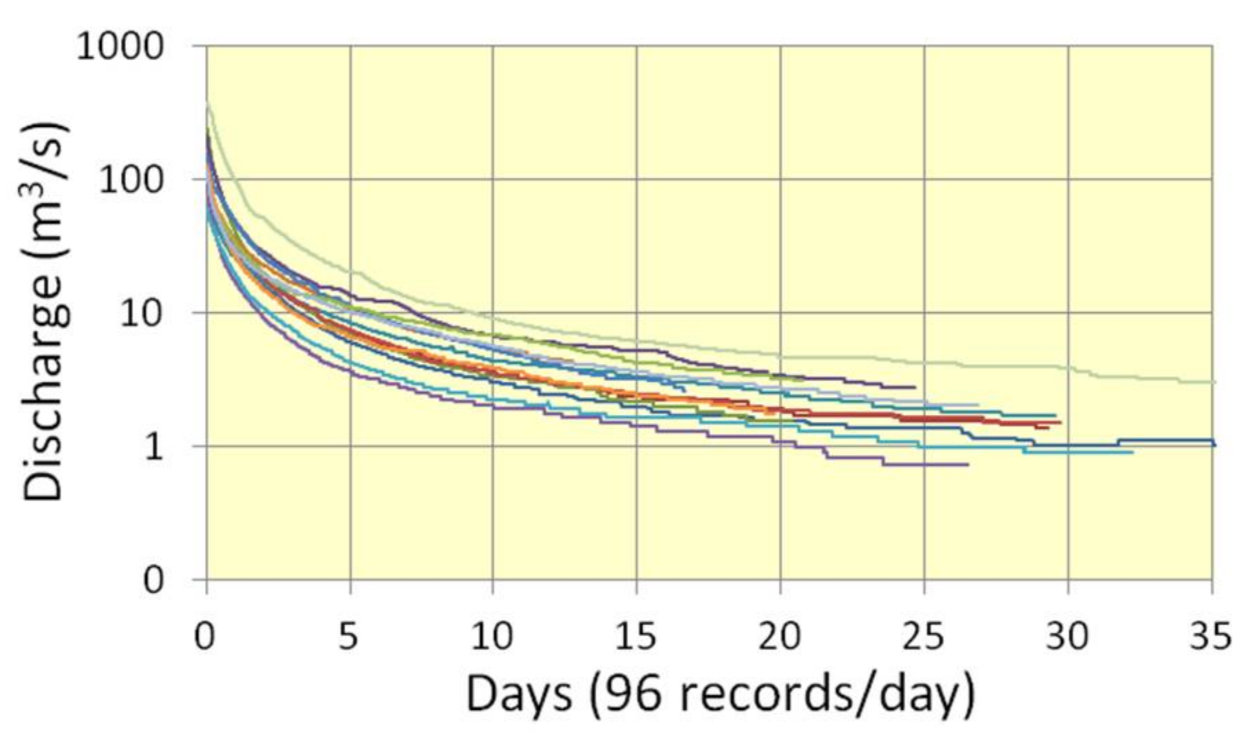
The study of hydrograph recession curves provides data regarding the structure and functions of different reservoirs present in a watershed [18,19,20,21]. Reference [22] uses non-linear reservoir algorithms supported by an analytical derivation. Reference [23] presents a new method for the analysis of the recession limb of a hydrograph, which differs from previous methods in that the time increment from which the slope is estimated is not held constant over the entire recession curve. Instead, the time step for each observation is properly scaled to the observed drop in discharge. Reference [24] performs a comparison between commonly used techniques for hydrograph recession analysis and a new approach based on wavelet transform and concludes that direct flow and the location of the base-flow component are easily determined through the wavelet maps.
Since 1930, rainfall-runoff models based on a combination of linear and non-linear reservoirs have been used in hydrology research. The linear reservoir model of Reference [25] is one of the oldest and simplest models to simulate the rainfall–runoff relation. The linear reservoir model constitutes the basis for many conceptual models [26]. However, Reference [27] proposed a conceptual model composed of a cascade of linear reservoirs with equivalent storage coefficients. Reference [28] extended Nash’s model to include the transition effect between the flow and accounts for the concept of a linear canal. Because it is not easy to obtain an explicit expression for the UIH when establishing the rainfall distribution in the complex geomorphology of watersheds, simplified models have been proposed, such as the models in series (cascade) linear reservoirs presented by References [29,30].
There are numerous studies on hydrograph decomposition, recession behaviour and the distribution of recharge [31,32]. The recent work of Reference [33] are worth highlighting, as they introduce a quantitative approach to spring hydrograph decomposition by combining analytical and numerical solutions for diffusive flux and simulated spring hydrographs of synthetic karst systems. Early recession behaviour of spring hydrographs is investigated in Reference [34], who conclude that the exponential recession function represents a long-term approximation of analytical solutions for the flow in fissured matrix blocks. Also, an interpretation of the shape of several recession curves is provided by a more general fractal approach, which assumes that the catchment is composed of blocks of different sizes. Reference [35] develops a quantitative approach of the temporal distribution of recharge in karst systems based on spring hydrographs and provides a time-continuous approach for the estimation of inflow into the conduit system of a karst aquifer, which consists of the sum of direct recharge and flow from the fissured matrix blocks into the conduit system. Examples of a geomorphological approach for recession curves analysis are described in References [36,37], in which an attempt is made to estimate the water storage in the Basin. Reference [38] proposes a new method for base-flow separation and recession analysis—the bump and rise method (BRM) through tracers. The advantage of the BRM is that it specifically simulates the shape of the base-flow or pre-event component as shown by tracers.
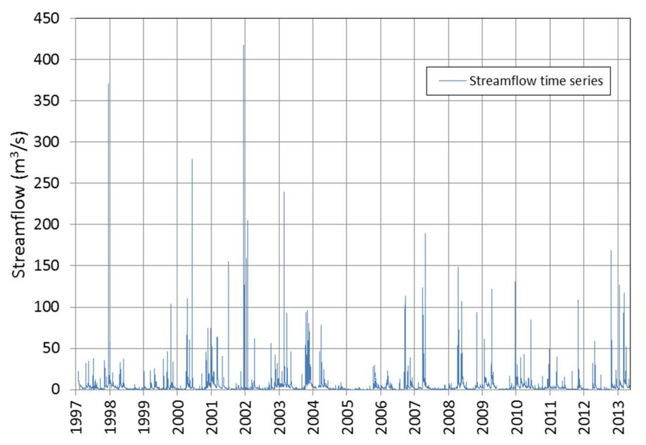
A new methodology for the separation of streamflow time series into flow components is developed in this article. The method is based on the Parallel Linear Reservoir models (PLR) and, more specifically, on the Dynamic Relations Equation (DRE) proposed in Reference [39], which has three highlights: (1) The proposed equation facilitates the calibration stage that, by using least squares adjustments, determines a single and optimal solution, unlike other methods that find compatible solutions but with the intervention of the user to obtain the parameters of the model. Such would be the case with logarithmic or graphical adjustments of the cell models; (2) Usually a two-component flow separation is established, quick and slow; but with PLR models there may be intermediate components that sometimes represent the actual reservoirs of the basins well; (3) Unlike other methodologies, with this one, if a flow component or the total discharge is known, the DRE allows the deduction of the other flow components as a single solution, without having to make estimates of flow sharing. This last feature makes PLR models useful for the simulation of certain hydrological processes, such as rainfall-runoff transformation and routing, at different parts of the basin. The separation of the flow components—the aim of the present article—will be framed within this last process.
The formulation originates from two classic equations—the discharge or storage equation and the continuity or water balance equation. In this article, an adaptation of this formulation is made to be applied to the separation of the base-flow from the continuous time series of total streamflow.
The main objective of this work is to present the PLR model as suitable for carrying out the base-flow separation from the time series of total discharge. For this purpose, the methodological development for the PLR modelling is presented based on the recession curves of the real hydrographs. Subsequently, the application of the model to a basin in the northeast of Spain is presented. In this work, the results of the PLR models are compared with the results of other models already diffused and accepted as those based on the Mathematical Digital Filtering Method. The work was performed using software developed by the authors of this article in the Department of Earth Sciences at the University of Zaragoza. The SHEE (Simulation of Hydrological Extreme Events) package is an adaptation of traditional hydrological models to DEMs and databases. It has resulted in several publications, including those related to hydrology [2,39,40,41,42,43,44,45,46], and it uses powerful libraries (e.g., OpenGL, GDI, GDAL, Proj4) for the management and display of DEM and datasets. Additionally, its interface provides rapid and high quality OPENGL graphics, in both RASTER and VECTOR formats.

2. Materials and Methods

2.1. Mathematical Digital Filtering Method

Mathematical Digital Filtering is a recursive digital filter method commonly used in signal analysis. Reference [47] proposes Equation (1), subject to Ft ≤ Qt. Reference [48] adapted the method for stream flow partitioning, making the assumption that low frequency base-flow could be distinguished from high frequency high flows and proposed Equation (2). References [49,50], with the collaboration of other authors, provide a fruitful trajectory on algorithms based on Digital Filters, with Equations (3) and (4) being two of the most widespread. The base-flow index (BFI) is the ratio of the base-flow volume (calculated from Ft) to the volume of streamflow (Qt) over a specified period. Reference [51] proposed the general form (Equation (5)) of a digital filter considering a digital filter parameter and BFImax (maximum value of long term BFI over a specified period).
F t = α   F t 1 +   1 α 2   ( Q t + Q t 1 )
F t = α   F t 1 +   1 + α 2   ( Q t Q t 1 )
F t = 3 α 1 3 α   F t 1 +   2 3 α   ( Q t α   Q t 1 )
F t = α 2 α   F t 1 +   1 α 2 α   Q t
F t = ( 1 BFI max )   α   F t 1 + ( 1 α ) BFI max   Q t 1 α   BFI max
where Ft is the quick-flow response at the tth sampling instant, Qt is the original streamflow at the tth sampling instant and α is the parameter that enables the shape of the separation to be modified.
B t = Q t F t
where Bt is the base-flow at the tth sampling instant. The filter is generally run through multiple times per dataset. For example, three passes are commonly used—forward, backward and forward.

2.2. Parallel Linear Reservoir Models

In the PLR models, for a given instant, the dynamic relations between the different deposits that compose a model are controlled by some of the forms of Equation (7) [39], where nr is the number of reservoirs (at other times they are known as cells and as deposits) that make up the model (usually works with models of 2 or 3 reservoirs); Qi is the discharge of the reservoir I, and Si is the storage. For a model of two reservoirs, one is the quick-flow and the other is the base-flow.
( Q 1 Q 01 ) 1 α 1 =     = ( Q i Q 0 i ) 1 α i =     = ( Q nr Q 0 nr ) 1 α nr
( S 1 S 01 ) 1 α 1 =     = ( S i S 0 i ) 1 α i =     = ( S nr S 0 nr ) 1 α nr
Q0i and αi are parameters of the model that are determined from the recession curves of the hydrographs. The αi parameter is called a depletion or recession coefficient and is also known as the response factor. Q0i is the flow for a given instant, being the same instant for all the Q0i. To be precise, there are nr-1 equations and since we are trying to find nr unknowns, another equation is needed—the mass conservation equation (Equation (8)).
Q t = i = 1 nr Q i
Once the model is calibrated, that is, once the parameters Q0i and αi are already known based on the streamflow records (Qt) of the time series, figuring out the Qi values of each reservoir through Equations (7) and (8) is needed, thus separating the quick-flow and the base-flow. Therefore, it is possible to propose a unique equation dependent on the discharge of one of the reservoirs (Equation (9)) with a single unknown, Q1.
Q t = i = 1 nr [ Q 0 i ( Q 1 Q 01 ) α i α 1 ]
Since it is a nonlinear equation, it can be solved by successive iterations by applying Taylor’s development to linearize the equation and solve it using the Newton-Raphson method (see Appendix A). Once Q1 is obtained through the set of Equation (7), the remaining Qi values can be obtained.
For a given instant, once the distribution of the discharge of each reservoir is known, Equation (10) can determine the storage (S) or natural water reserves of the entire basin and the available water reserves in each reservoir.
S t = i = 1 nr S i   = i = 1 nr Q i α i

2.3. Calibration of the Parallel Linear Reservoir Models

In order to be able to use the methodology described in the previous section, it is necessary to establish the Linear Reservoir Model, that is, to adjust the parameters Q0i and αi to the actual recession curves of the time series of total streamflow.
The recession curves are therefore hydrograph sections conditioned by the release of water from natural reservoirs, that is, they are the result of the sum of the multiple contributions from natural reservoirs. To calibrate the model (i.e., to obtain the Q0i and αi parameters), segments from the recession curve are selected from an actual hydrograph. These segments can be individually or collectively analysed to understand the processes that generate the flow. To obtain a solution for these segments, a graphical approach is traditionally adopted. However, recently analysis has involved the definition of an analytical solution or a mathematical model that can properly fit the recession segments. Reference [39] developed a completely automatic method that is based on adjustment via the least squares method, combining the Reference [12] equation with Equation (7) of this paper.

2.4. Case Study of the Continuous Streamflow Time Series of a Catchment

The application of the described methodology was carried out with the streamflow time series (Figure 1) of the Alcanadre River in the stream gauge A033 of the Spanish Hydrological Information Automatic System (SAIH). The records of the series were set every 15 min, beginning on 27 January 1997 and ending on 14 May 2013, which accounts for about 568,000 records.
The Alcanadre river basin is a part of two geological domains: the Pyrenean domain of the Jaca-Pamplona syncline to the north and the domain of the middle basin of the Ebro River to the south, separated by an important tectonic structure called the Surpirenaic frontal thrusts system. The most abundant materials of the Pyrenean domain in the basin are the Miocene conglomerates and clays, Eocene sandstones and the limestone and outcrops of upper Cretaceous limestones. These materials are folded and have faults, mainly in the N-S direction. In the Ebro basin, we find conglomerates, sandstones and marls and, in the South, Gypsum of the Miocene with valley bottoms of conglomerates, gravels and clays of the Quaternary. These materials have a practically horizontal layout.
The main materials that constitute aquifers in the Alcanadre river basin are the limestones and conglomerates of the Miocene and Eocene that appear in the Sierra de Guara and the conglomerates of the marginal zone of the Ebro basin While being less important than the previous aquifers, it is possible to emphasize the existence of quaternary aquifers created from alluvial deposits of the rivers and the extensive and low-thickness deposits of gravels and clays that constitute glacis.
In Figure 2, the catchment is presented with its water divide and a geological synthesis, the altimetry distribution and the isohyets of annual precipitation. As can be seen, the northern zone is the main zone for the recharge of aquifers, due to it being the one with the highest precipitation and where calcareous formations—which represent the origin of the main aquifers of the basin—outcrop. In Table 1, some characteristics of the basin are presented.
In relation to this basin, there are important antecedents among which we highlight the work of Reference [52], which performed an analysis of the recession curves of the rivers Alcanadre and Guatizalema to perform a hydrodynamic characterization of carbonated aquifers. This is related to the dynamic volume of the basin with the streamflow of the rivers, which allows us to make its corresponding streamflow recession theoretical curve.

3. Results

3.1. Setting PLR Models

To set the Reservoir Models, the 14 recession curves shown in Figure 3 were selected. The adjustment methodology applied resulted in the parameters shown in Table 2 and Table 3 for the 14 curves. The adjustment has been made for two models, a two reservoirs model (2R model) and a three reservoirs model (3R model).
Figure 4 shows the parameters obtained in the 14 recession curves, expressed in logarithmic scales, −Ln(α) versus −Ln(Q0). In the case of the 3R model, the parameters of the 14 recession curves are aligned. Each model is the best fit for a particular recession curve but it is necessary to establish a generic model applicable to the complete time series. The mean of all the parameters of each model is the result yielding the best fit by the least squares method and approaching the regression line. Table 2 and Table 3 show the parameters for the generic 2R model and the 3R model, respectively. The squared Pearson’s correlation coefficient (R2), with respect to the linear regression line, is 0.789 for the 2R Model and 0.934 for the 3R model.

3.2. Flow Separation with PLR Models

With the Q0 y α parameters of the generic models described in Table 2 and Table 3, flow separation in each reservoir for the continuous time series of the stream gauge A033 was performed. The series extends temporarily from 1987 to 2013, with data recorded every 15 min. In Figure 5 and Figure 6, six stretches of the hydrograph of the time series are represented.
The base-flow predicted by the 3R model is smaller than that of the 2R model but the 3R model takes into account an intermediate reservoir that has a notable influence on the regulation of the basin. From a purely mathematical point of view, both the 2R and 3R models can be adjusted to the real recession curves with great performance, but in terms of conventional concepts of base flow separation, the 3R model appears to be more plausible than the 2R model in this particular catchment due to its characteristics and especially due to the development of a karst area in the head zone. This basin could be described with three flow components: a fast one, corresponding to the superficial flow, which possesses great relevance during the river floods; an intermediate flow, which corresponds mainly to the circulation of the larger karstic galleries; and a third, slow flow, which would correspond to the circulation through the joints, fissures, smaller diaclases and to the aquifers developed in granular soils in the alluvial terraces of the river.

3.3. Flow Separation with Mathematical Digital Filter

Simulations were performed with the Mathematical Digital Filter models of Equations (1)–(5) and it has been verified that the differences between them are not as relevant as the differences between the PLR models. This is the reason why only one single Digital filter model was represented, the one corresponding to the equation in Reference [49], due to it being one of the most widespread. Figure 7 shows the flow separation results for the six stretches. The digital filter model only allows separation of the base stream without considering an intermediate flow.

3.4. Efficiency Analysis

In order to compare the proposed reservoir models, a benchmarking analysis of the base flow obtained with the classic filter model and with the 2R model has been carried out. The results of this study for the six stretches are in Table 4.
Several indices have been used: the Nash–Sutcliffe efficiency coefficient [53], the index of agreement (IOA), the correlation coefficient of the Pearson product between the observed and calculated data (R), the coefficient of determination (R2), the root mean square error (RMS, RMSE or EMC), the ratio of absolute error of peak flow (RAE), the Nash–Sutcliffe efficiency coefficient with logarithmic values (lnNSE), the Relative efficiency criteria of the Nash–Sutcliffe coefficient (NSErel), the Relative efficiency criteria of the index of agreement (IOArel), the weighted coefficient of determination (wR2) and the percent bias (pBIAS). The meaning of these parameters and their equations can be found in Reference [39] and for pBIAS in Reference [54].
On the other hand, in order to compare these results with similar studies, Reference [55] made a benchmarking with the NSE and pBIAS indices, with the results obtained with baseflow separation methods, versus physically based models. The study is carried out with eight main scenarios where two kinds of terrain, sandy and silt-sandy, three different states of the groundwater level and the presence of several water pumping scenarios from the aquifer are contemplated. The results obtained have a high range of variation. For NSE, they obtained values between 0.1 and 0.9. In our study, we obtained 0.344 for stretch 1 and values of around 0.8 for the other stretches. With pBIAS, these authors obtained values between −16% and +34%. In our case, we obtained negative values in stretches 3, 4 and 6, with a minimum value of −5.1% and a maximum value of 25.5% in Section 1.

4. Discussion

The equation of Dynamic Relations between deposits (Equation (7), [39]) allows for the establishment of continuous streamflow separation models in two or more flow components, quick-flow, base-flow and intermediate flows for other cases. These models are calibrated with very few parameters (Q0i and αi), thus they are parsimonious models, which fit the recession curves of the real hydrographs of the streamflow time series.
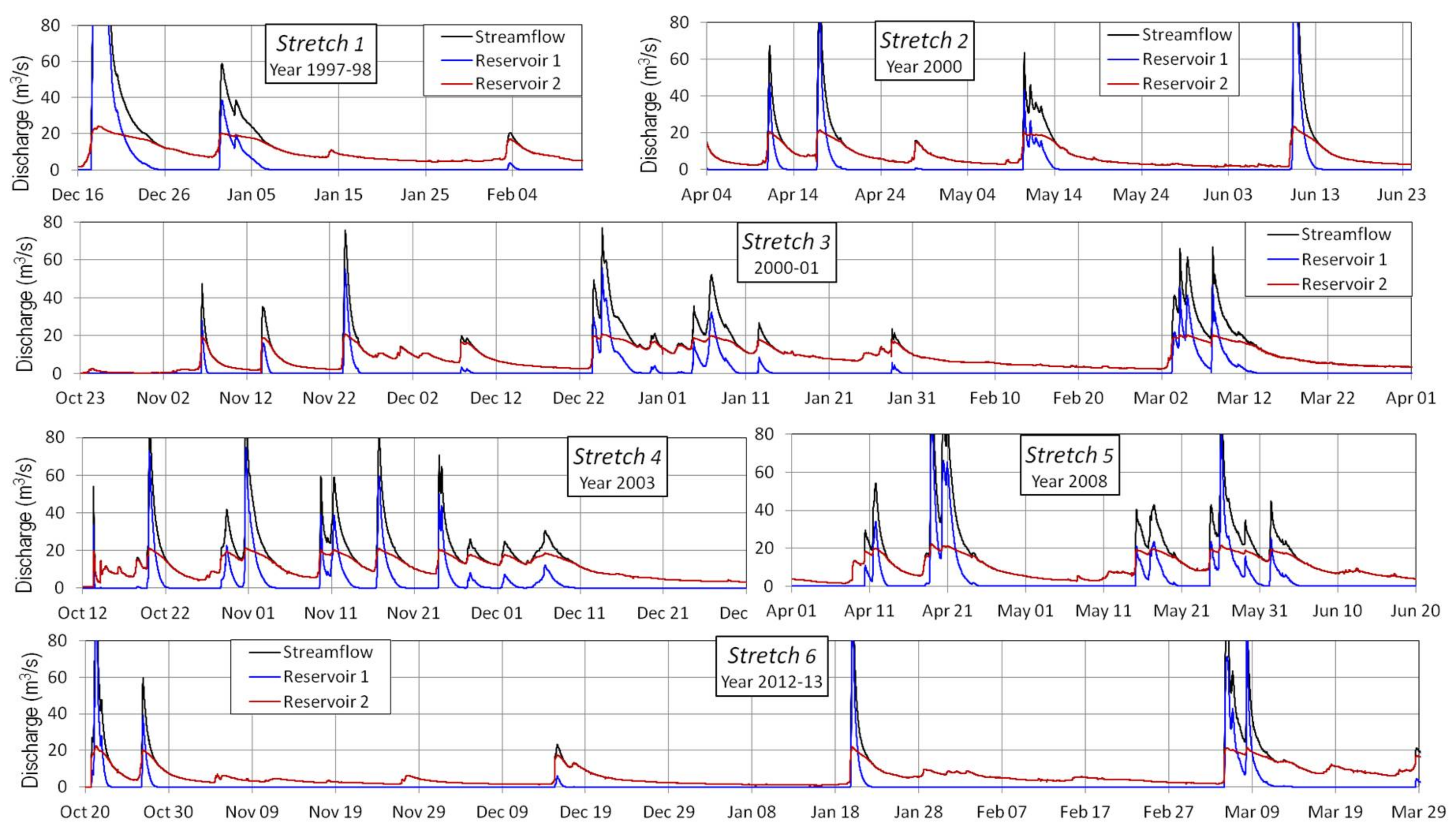
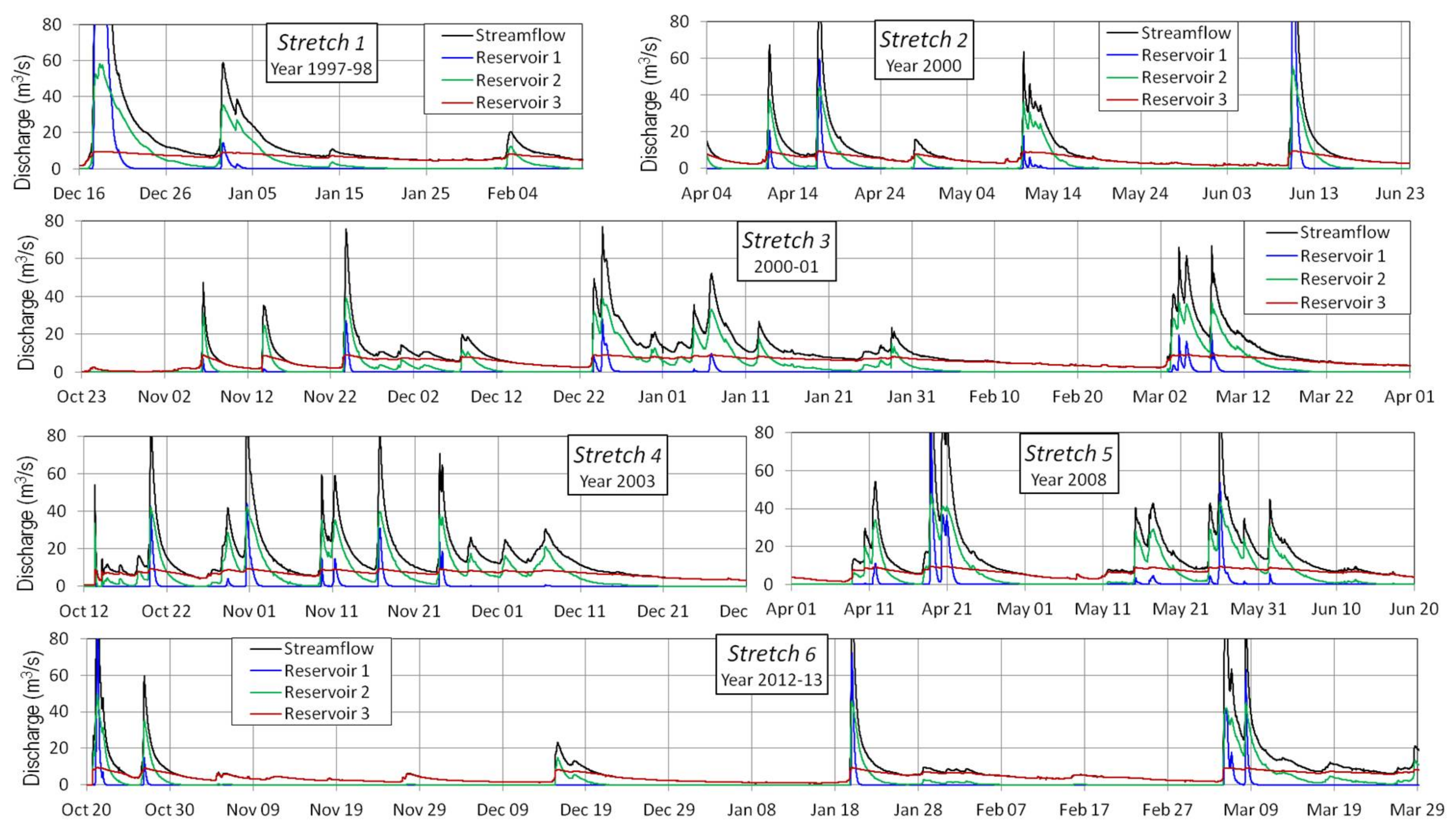
 Figure 5 and Figure 6 show the flow separation results for the 2R and 3R models and Figure 7 describes the results for the filter model of Reference [49].

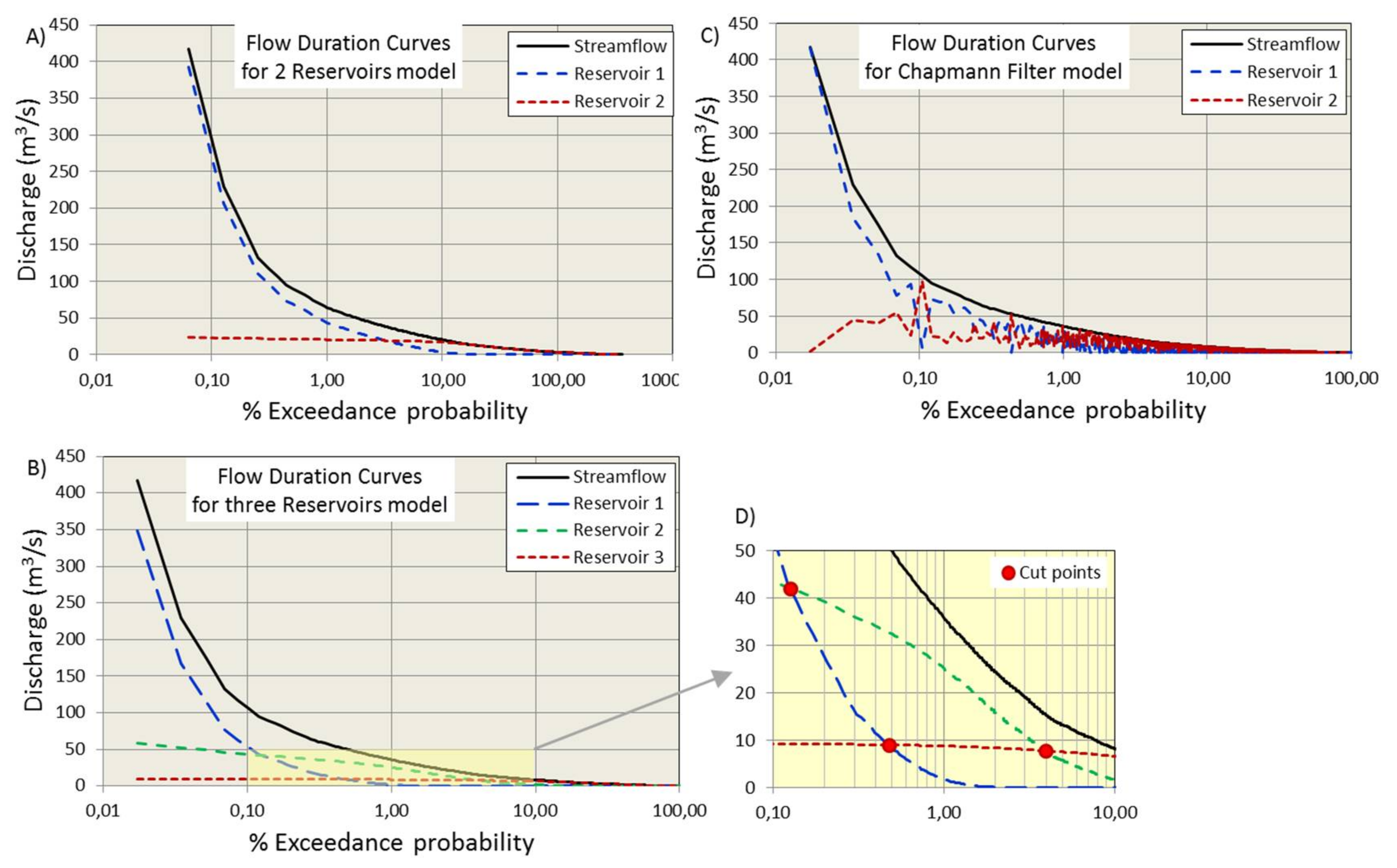
4.1. Flow Duration Curves

Based on the complete time series and the flow separation results, Figure 8 shows the Flow Duration Curves (FDCs) for the three models, which are cumulative frequency curves that show the percentages of time during which specified discharges were equal or were exceeded in given periods (exceedance probability). FDCs represent the flow characteristics of a stream throughout its range of variation [38]. FDCs can also be determined for the separated stream components, thus allowing the assessment of the characteristics of each flow component and therefore the characteristics of the natural deposits of the basin assigned to each stream.
In order to establish the FDCs, the streamflow values were ordered from highest to lowest and accompanied by the flow components associated with each streamflow value. As can be seen, for the mathematical filter model, the values of the associated flows do not keep a good correlative distribution in terms of order.
On the other hand, flow duration curves for streamflow, base-flow, quick-flow and intermediate flow all follow a decreasing distribution. The differences between the curves of each flow component are evident. The quick-flow duration curve (QFDC) decreases very quickly compared to the base-flow duration curve (BFDC), which decreases more slowly. The QFDC has very high values at the beginning but most of the time presents values lower than those of the BFDC. The curves of each component are cut at certain points—at one point for the 2R model and at three points for the 3R model.
Figure 8D shows the cut-off points for the 3R model in detail and Table 5 presents the cut-off values for the two PLR models. Within a 0.13% to 3.94% range (0.46 to 14.39 days/year), the intermediate reservoir is the one contributing the most to the total streamflow of the river. Only at 0.46 days/year and coinciding with flood episodes of the river, it is the quick reservoir that contributes the bigger discharge. However, it is the base-flow reservoir that contributes more for most of the time—about 350 days/year.

4.2. Contribution of Each Flow Component to the Total Streamflow

If FDCs are integrated, the water volume supplied by each flow component to the total streamflow can be obtained. Table 6 shows the results expressed as average annual volume and as a percentage of each reservoir over the total streamflow. For the 3R model it follows that, for the Alcanadre river at the A033 gauging station, the annual average streamflow is 117 hm3/year, of which 8 hm3 circulate through the quick reservoir, 33 hm3 circulate through the intermediate reservoir and 76 hm3 flow through the base flow reservoir.
With all these data, the importance of the slow reservoir for two aspects is highlighted: the first aspect is regarding the annual volume of water circulating for the basin—76 hm3—which represents 65% of the total streamflow, while the second aspect refers to the capacity of regulation of the water resource available in the basin and distributed during most of the time, which for 350 days/year represents the main contribution to surface water.

4.3. Availability of Water Resources in the Catchment and Residence Time

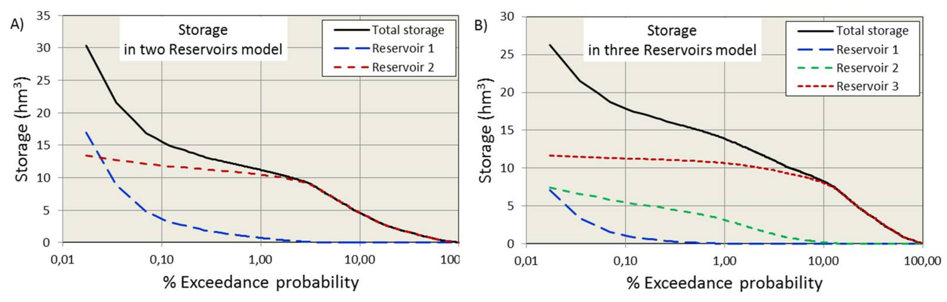
In addition to the FDCs discussed above, Equation (10) also provides Storage Duration Curves (SDCs), which represent cumulative frequency curves that show the percentage of time during which specified availability of water resources were equalled or exceeded in given periods (exceedance probability). Figure 9 shows these curves for the two PLR models and, from them, interesting information can be extracted. The storage in the slow reservoir has two well-differentiated phases, one characterized by the other reservoirs being active and the other one, a longer one, when the other reservoirs have no influence.
Table 7 shows the maximum, minimum and mean values of discharge and storage for each reservoir. The volume of water stored in a watershed that is susceptible to influence the flow of the river is known as dynamic storage (DS) and can be estimated as the difference between the maximum and minimum storage. For the 3R model, the DS is 23 hm3, with a distribution of 7.1, 7.3 and 8.7 hm3 respectively for quick, middle and slow reservoirs, respectively.
Water availability in each deposit varies with time. During flood episodes, reservoir recharge occurs and when the rains cease, the reservoirs discharge at different velocities. The total storage for each time step is different for each model because it is the sum of the storage of each reservoir and is calculated by Equation (10) from the discharge (Qi) of each reservoir.
The mean storage (MS) represents the average availability of the water resource along the complete time series. The 3R model has a mean storage of 0.01, 0.13 and 2.91 hm3 for reservoirs 1, 2 and 3, respectively, which again indicates that the main water guarantee comes from the slow reservoir.
The mean discharge (MD) represents the average flow throughout the year and is calculated as the continuous flow for a year required for discharging the annual volume. Note that mean storage and mean discharge do not correlate between models, with the maximum value of the mean storage for the slow reservoir of the 3R model being 2.91 hm3 and the maximum value of mean discharge for the slow reservoir of the 2R model being 3.05 m3/s.
Residence time (RT) or removal time can be calculated from the above variables with Equation (11) and represents the average amount of time spent by the flow of water in each reservoir.
RT   ( days ) = MS   ( m 3 ) MD ( m 3 / day )  
So, for the 3R model, the residence time is 0.24, 1.45 and 14.03 days for the reservoirs quick to slow, respectively.
The storage for each reservoir can also be calculated from the FDCs, as shown in Table 8. Note that at the cut-off points, in two of the tanks, the same flow rate is discharged but the storage differs considerably.

5. Conclusions

In this work, a new method for base-flow separation based on Parallel Linear Reservoir models is proposed. The Dynamic Relations equation sets up a single and optimal solution for the parameters that govern the Parallel Linear Reservoir models. With these models, more than two flow components can be established to assess the water routing through the basin. The Flow Duration Curves allow evaluation of the dynamic relations between flow components that circulate through the labyrinths of the hydrological cycle of the basin. The Storage Duration Curves allow assessment of the temporary availability of the water resources in the basin.
This article demonstrates the suitability of the PLR models and the equations that describe them, to elaborate models of continuous development for the separation of different flows from the total streamflow recorded in gauged stations. Based on the assessment of the results of the PLR models, through flow duration curves (FDCs) and other techniques, evaluations can be made about the dynamic relations between different components of the flow, the recharge of aquifers and the state of the water resources of the basins.
The developed methodology has interesting specific characteristics and a series of properties that makes it suitable for such purposes, among which we can highlight the following:
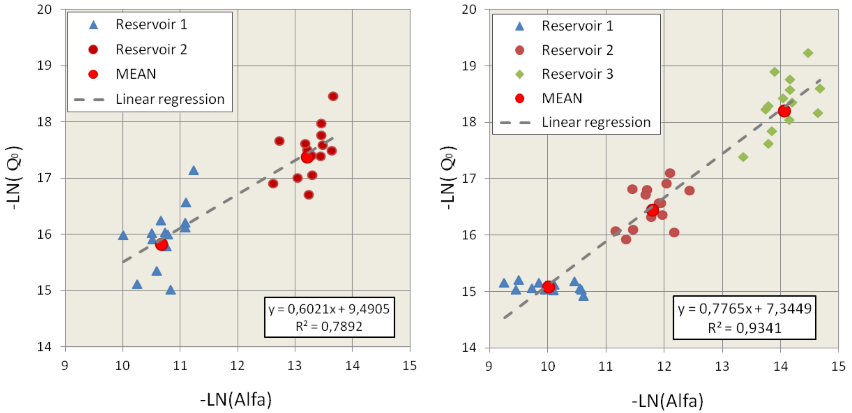
Calibration of model parameters, based on actual recession curves recorded in the hydrographs of gauging stations. The proposed formulation allows adjustment of the parameters of the models with a single optimal solution, derived from a least squares adjustment, unlike other techniques in which it is necessary to manually intervene in the adjustment. This makes the results of the PLR models conform to the real hydrographs, especially in the recession stretches, as demonstrated in the study of actual episodes carried out in Reference [39].
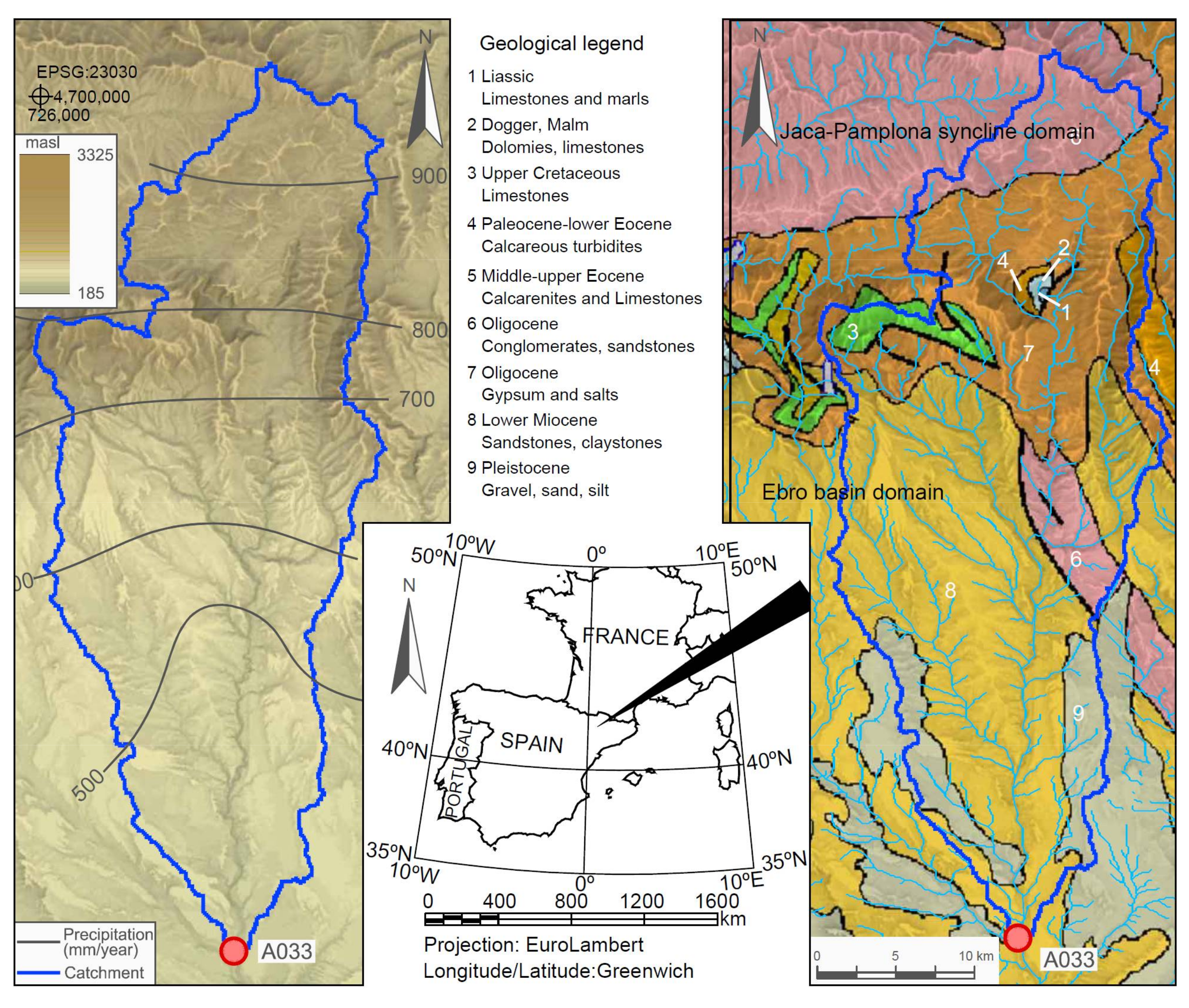
Models with more than two flow components can be established. In the example proposed for the Alcanadre River in Spain, three components better reflect the actual response of the basin, in the upper zone of which a large karst system is developed. In this area, the main recharge of fracturing aquifers developed in the carbonate formations (ages between the upper Cretaceous and the Eocene) that outcrop in the more elevated parts of the catchment takes place.
In addition to the separation between the different flow components, the PLR models with the proposed formulation allow the investigation and evaluation of the dynamic relations between the different components and also the drawing of conclusions about their state in each moment, the volumes stored in each reservoir, the discharges over time, the water reserves in each reservoir and the entire basin, the detractions of the aquifer flow and its recharge, the average residence time of the water volume, the volume of contribution of each type of reservoir, and so forth.
Special mention must be made of the state of water resources in the basin. In the example of the Alcanadre River in Spain, relevant information has been obtained, which can be used for watersheds in other places by following the methodology set out in this paper. For example, the importance of the slow reservoir in terms of water supply, which accounts for 65% of the total contribution, is considered quantitatively and, in terms of water reserves and water-regulation guarantee, is equivalent to a reservoir with 26 hm3 of capacity.

Acknowledgments

This work has been partially subsidized by the Research Group, “Analysis of Continental Sedimentary Basins” of the Government of Aragon and FEDER Funds for which we are grateful.

Author Contributions

All authors conceived and designed the experimental work, with special mention to J. Castillo-Mateo for having completed the mathematical development allowing its applicability to the real cases of the Alcanadre River.

Conflicts of Interest

The authors declare no conflict of interest.

Appendix A

The equation to be solved is Equation (9), with a single unknown, Q1. In order to simplify the equation, the terms with constant values are grouped:
f ( Q 1 )   = Q t +   i = 1 nr m i Q 1 p i
were
p i = α i α 1
and
m i = Q 0 i Q 01 p i
The first derivative of the function is:
f ( Q 1 )   =   i = 1 nr p i m i Q 1 p i 1
And, therefore, for iteration k, the corrected value is as follows:
Q 1 k = Q 1 k 1   f ( Q 1 k 1 ) f ( Q 1 k 1 )
and so, through successive iterations, we arrive at the solution.

References

  1. Fekete, B.M.; Looser, U.; Pietroniro, A.; Robarts, R.D. Rationale for Monitoring Discharge on the Ground. J. Hydrometeorol. 2012, 13, 1977–1983. [Google Scholar] [CrossRef]
  2. Mateo-Lázaro, J.; Sánchez-Navarro, J.A.; García-Gil, A.; Edo-Romero, V. Flood Frequency Analysis (FFA) in Spanish catchments. J. Hydrol. 2016, 538, 598–608. [Google Scholar] [CrossRef]
  3. Lacasta, A.; Morales-Hernández, M.; Murillo, J.; García-Navarro, P. GPU implementation of the 2D shallow water equations for the simulation of rainfall/runoff events. Environ. Earth Sci. 2015. [Google Scholar] [CrossRef]
  4. Guo, W.; Wang, C.; Zeng, X.; Ma, T.; Yang, H. Quantifying the spatial variability of rainfall and flow routing on flood response across scales. Environ. Earth Sci. 2015, 74. [Google Scholar] [CrossRef]
  5. Beskow, S.; de Mello, C.R.; Vargas, M.M.; De Lima-Correa, L.; Caldeira, T.L.; Duraes, M.; Sanchonete-Aguilar, M. Artificial intelligence techniques coupled with seasonality measures for hydrological regionalization of Q90 under Brazilian conditions. J. Hydrol. 2016, 541. [Google Scholar] [CrossRef]
  6. Rahmati, O.; Haghizadeh, A.; Stefanidis, S. Assessing the Accuracy of GIS-Based Analytical Hierarchy Process for Watershed Prioritization; Gorganrood River Basin, Iran. Water Resour. Manag. 2016, 30, 1131–1150. [Google Scholar] [CrossRef]
  7. Barberá, J.A.; Andreo, B. River-spring connectivity and hydrogeochemical interactions in a shallow fractured rock formation. The case study of Fuensanta river valley (Southern Spain). J. Hydrol. 2017, 547, 253–268. [Google Scholar] [CrossRef]
  8. Moore, R.D. Storage-outflow modelling of streamflow recessions, with application to a shallow-soil forested catchment. J. Hydrol. 1997, 98, 260–270. [Google Scholar] [CrossRef]
  9. Griffiths, G.A.; Clausen, B. Streamflow recession in basins with multiple water storages. J. Hydrol. 1997, 190, 60–74. [Google Scholar] [CrossRef]
  10. Dewandel, B.; Lachassagne, P.; Bakalowicz, M.; Weng, P.H.; Al-Malki, A. Evaluation of aquifer thickness by analysing recession hydrographs. Application to the Oman ophiolite hard-rock aquifer. J. Hydrol. 2003, 274, 248–269. [Google Scholar] [CrossRef]
  11. Boussinesq, J. Essai Sur la Theories des Eaux Courantes; Memoires presentes par divers savants a l’Academic des Sciences de l’Institut National de France: Paris, France, 1877. [Google Scholar]
  12. Maillet, E. Essais D’hydraulique Souterraine et Fluviale; Librairie Science Hermann Paris: Paris, France, 1905. [Google Scholar]
  13. Thomas, M.P.; Cervione, M.A. A proposed streamflow data program for Connecticut. Conn. Water Resour. Bull. 1970, 23. [Google Scholar]
  14. Tasker, G.D. Estimating low flow characteristics of streams in southeastern Massachusets from maps of groundwater availability. US Geol. Surv. Prof. Pap. 1972, 800, 217–220. [Google Scholar]
  15. Parker, G.W. Methods for Determining Selected Flow Characteristics for Streams in Maine; US Geological Survey Open-File Reports; USGS: Reston, VA, USA, 1977; pp. 78–871.
  16. Vogel, R.M.; Kroll, C.N. Regional geohydrologic-geomorphic relationships for the estimation of low-flow statistics. Water Resour. Res. 1992, 28, 2451–2458. [Google Scholar] [CrossRef]
  17. Woods, R. The relative roles of climate, soil, vegetation and topography in determining seasonal and long-term catchment dynamics. Adv. Water Resour. 2003, 26, 295–309. [Google Scholar] [CrossRef]
  18. Mijatovic, B. Détermination de la transmissivité et du coefficient d’emmagasinement par la courbe de tarissement dans les aquifêres karstiques. Int. Assoc. Hydrogeol. 1974, 10, 225–230. [Google Scholar]
  19. Brutsaert, W.; Nieber, J.L. Regionalized drought flow hydrographs from a mature glaciated plateau. Water Resour. Res. 1977, 34, 233–240. [Google Scholar] [CrossRef]
  20. Troch, P.; De Troch, F.; Brusaert, W. Effective water table depth to describe initial conditions prior to storm rainfall in humid regions. Water Resour. Res. 1993, 29, 427–434. [Google Scholar] [CrossRef]
  21. Szilagy, J.; Parlange, M.B.; Albertson, J.D. Recession flow analysis for aquifer parameter determination. Water Resour. Res. 1998, 37, 1851–1857. [Google Scholar] [CrossRef]
  22. Wittenberg, H. Baseflow recession and recharge as nonlinear storage processes. Hydrol. Process. 1999, 13, 715–726. [Google Scholar] [CrossRef]
  23. Rupp, D.E.; Selker, J.S. Information, artifacts, and noise in dQ/dt—Q recession analysis. Adv. Water Resour. 2006, 29, 154–160. [Google Scholar] [CrossRef]
  24. Sujono, J.; Shikasho, S.; Hiramatsu, K. A comparison of techniques for hydrograph recession analysis. Hydrol. Process. 2004, 18, 403–413. [Google Scholar] [CrossRef]
  25. Zoch, R.T. On the relation between rainfall and streamflow. Mon. Weather Rev. 1934, 62, 315–322. [Google Scholar] [CrossRef]
  26. Chow, V.T.; Maidment, D.R.; Mays, L.W. Applied Hydrology; McGraw-Hill: New York, NY, USA, 1988. [Google Scholar]
  27. Nash, J.E. The form of the instantaneous unit hydrograph. IASH Publ. 1957, 45, 114–121. [Google Scholar]
  28. Dooge, J.C.I. A general theory of the unit hydrograph. J. Geophys. Res. 1959, 64, 241–256. [Google Scholar] [CrossRef]
  29. Wang, G.T.; Chen, S. A linear spatially distributed model for a surface rainfall–runoff system. J. Hydrol. 1996, 185, 183–198. [Google Scholar] [CrossRef]
  30. Jeng, R.I.; Coon, G.C. True form instantaneous unit hydrograph of linear reservoirs. J. Irrig. Drain. Eng. ASCE 2003, 129, 11–17. [Google Scholar]
  31. McCuen, R.H. Hydrologic Analysis and Design; Prentice Hall: Upper Saddle River, NJ, USA, 1989; pp. 355–360. [Google Scholar]
  32. Arnold, J.G.; Allen, P.M. Validation of automated methods for estimating baseflow and groundwater recharge from stream flow records. J. Am. Water Resour. Assoc. 1999, 35, 411–424. [Google Scholar] [CrossRef]
  33. Kovács, A.; Perrochet, P. A quantitative approach to spring hydrograph decomposition. J. Hydrol. 2008, 352, 16–29. [Google Scholar] [CrossRef]
  34. Birk, S.; Hergarten, S. Early recession behaviour of spring hydrographs. J. Hydrol. 2010, 387, 24–32. [Google Scholar] [CrossRef]
  35. Geyer, T.; Birk, S.; Liedl, R.; Sauter, M. Quantification of temporal distribution of recharge in karst systems from spring hydrographs. J. Hydrol. 2008, 348, 452–463. [Google Scholar] [CrossRef]
  36. Biswal, B.; Marani, M. ‘Universal’ recession curves and their geomorphological interpretation. Adv. Water Resour. 2014, 65, 34–42. [Google Scholar] [CrossRef]
  37. Biswal, B.; Kumar, N. Estimation of ‘drainable’ storage—A geomorphological approach. Adv. Water Resour. 2015, 77, 37–43. [Google Scholar] [CrossRef]
  38. Stewart, M.K. Promising new baseflow separation and recession analysis methods applied to streamflow at Glendhu Catchment, New Zealand. Hydrol. Earth Syst. Sci. 2015, 19, 2587–2603. [Google Scholar] [CrossRef]
  39. Mateo-Lázaro, J.; Sánchez-Navarro, J.A.; García-Gil, A.; Edo-Romero, V. A new adaptation of linear reservoir models in parallel sets to assess actual hydrological events. J. Hydrol. 2015, 524, 507–521. [Google Scholar] [CrossRef]
  40. Mateo-Lázaro, J.; Sánchez-Navarro, J.A.; García-Gil, A.; Edo-Romero, V. Developing and programming a watershed traversal algorithm (WTA) in GRID-DEM and adapting it to hydrological processes. Comput. Geosci. 2013, 51, 418–429. [Google Scholar] [CrossRef]
  41. Mateo-Lázaro, J.; Sánchez-Navarro, J.A.; García-Gil, A.; Edo-Romero, V. Sensitivity analysis of main variables present on flash flood processes. Application in two Spanish catchments: Arás and Aguilón. Environ. Earth Sci. 2014, 71, 2925–2939. [Google Scholar] [CrossRef]
  42. Mateo-Lázaro, J.; Sánchez-Navarro, J.A.; García-Gil, A.; Edo-Romero, V. 3D-geological structures with digital elevation models using GPU programming. Comput. Geosci. 2014, 70, 147–153. [Google Scholar] [CrossRef]
  43. Mateo-Lázaro, J.; Sánchez-Navarro, J.A.; García-Gil, A.; Edo-Romero, V.; Castillo-Mateo, J. Modelling and layout of drainage-levee devices in river sections. Eng. Geol. 2016, 214, 11–19. [Google Scholar] [CrossRef]
  44. García-Gil, A.; Vázquez-Suñé, E.; Sánchez-Navarro, J.A.; Mateo-Lázaro, J. Recovery of energetically overexploited urban aquifers using Surface water. J. Hydrol. 2015, 531, 602–611. [Google Scholar] [CrossRef]
  45. García-Gil, A.; Vázquez-Suñé, E.; Sánchez-Navarro, J.A.; Mateo-Lázaro, J.; Alcaraz, M. The propagation of complex flood-induced head wavefronts through a heterogeneous alluvial aquifer and its applicability in groundwater flood risk management. J. Hydrol. 2015, 527, 402–419. [Google Scholar] [CrossRef]
  46. García-Gil, A.; Epting, J.; Garrido, E.; Vázquez-Suñé, E.; Mateo-Lázaro, J.; Sánchez Navarro, J.A.; Huggenberger, P.; Marazuela Calvo, M.A. A city scale study on the effects of intensive groundwater heat pump systems on heavy metal contents in groundwater. Sci. Total Environ. 2016, 572, 1047–1058. [Google Scholar] [CrossRef] [PubMed]
  47. Lyne, V.D.; Hollick, M. Stochastic Time-Variable Rainfall-Runoff Modeling. In Proceedings of the Hydrology and Water Resources Symposium, Perth, Australia, 10–12 September 1979; pp. 89–92. [Google Scholar]
  48. Nathan, R.J.; McMahon, T.A. Evaluation of Automated Techniques for Baseflow and Recession Analysis. Water Resour. Res. 1990, 26, 1465–1473. [Google Scholar] [CrossRef]
  49. Chapman, T.G. Comment on “Evaluation of automated techniques for base-flow and recession analyses” by R. J. Nathan and T. A. McMahon. Water Resour. Res. 1991, 27, 1783–1784. [Google Scholar] [CrossRef]
  50. Chapman, T.G.; Maxwell, A. Baseflow Separation—Comparison of Numerical Methods with Tracer Experiments. In Proceedings of the 23rd Hydrology and Water Resources Symposium, Hobart, Australia, 21–24 May 1996; pp. 539–545. [Google Scholar]
  51. Eckhardt, K. How to construct recursive digital filters for base flow separation. Hydrol. Process. 2005, 19, 507–515. [Google Scholar] [CrossRef]
  52. Sánchez, J.A.; Martínez, F.J.; De Miguel, J.L.; San Román, J. Los acuíferos carbonatados del macizo de Guara, análisis e interpretación de la curvas de recesión de caudales de los ríos que drenan. Rev. Acad. Cienc. Zaragoza 1988, 213–222. [Google Scholar]
  53. Nash, J.E.; Sutcliffe, J.V. River flow forecasting through conceptual models. Part I: A discussion of principles. J. Hydrol. 1970, 10, 282–290. [Google Scholar] [CrossRef]
  54. Gupta, H.V.; Sorooshian, S.; Yapo, P.O. Status of automatic calibration for hydrologic models: Comparison with multilevel expert calibration. J. Hydrol. Eng. 1999, 4, 135–143. [Google Scholar] [CrossRef]
  55. Partington, D.; Brunner, P.; Simmons, C.T.; Werner, A.D.; Therrien, R.; Maier, H.R.; Dandy, G.C. Evaluation of outputs from automated baseflow separation methods against simulated baseflow from a physically based, surface water-groundwater flow model. J. Hydrol. 2012, 458–459, 28–39. [Google Scholar] [CrossRef]
Figure 1. Time series of the A033 stream gauge of the Alcanadre River.
Water 10 00465 g001
Figure 2. Study area with the water divide of the catchment, altimetry shade with Ski View Factor algorithm, geological synthesis and drainage network.
Water 10 00465 g002
Figure 3. Recession curves (14) selected for the calibration of parameters.
Water 10 00465 g003
Figure 4. Calibration parameters, Q0 and α, of the 14 recession curves for the 2R and 3R models.
Water 10 00465 g004
Figure 5. Calibration Flow separation for the six stretches selected of the time series with the 2R model.
Water 10 00465 g005
Figure 6. Flow separation for the six stretches selected of the time series with the 3R model.
Water 10 00465 g006
Figure 7. Flow separation for the six stretches selected of the time series with the Filter model.
Water 10 00465 g007
Figure 8. Flow duration curves (FDCs) for two reservoir (2R), three reservoir (3R) and Filter model; (A) flow duration curves for two reservoirs model; (B) flow duration curves for three reservoirs model; (C) flow duration curves for Chapmann Filter model; (D) the cut-off points for the 3R model in detail.
Water 10 00465 g008
Figure 9. Storage duration curves (SDCs) for the 2R and 3R models. The storage represents the availability of water resources in the catchment; (A) storage in two reservoirs model; (B) storage in three reservoirs model.
Water 10 00465 g009
Table 1. Main characteristics of the Alcanadre catchment.
CharacteristicValueUnit
Area765km2
Main channel length69km
Main channel slope1.96%
Mean slope of the catchment16.84%
Mean slope of the network of DEM20.26%
SCS-Curve Number73
Table 2. Parameters of the models of two deposits.
Curveα1α2Q01Q02
11.96 × 10−51.78 × 10−63.015 × 10−75.553 × 10−8
21.52 × 10−51.42 × 10−69.965 × 10−81.564 × 10−8
32.17 × 10−51.83 × 10−61.092 × 10−72.498 × 10−8
43.53 × 10−53.31 × 10−62.724 × 10−74.573 × 10−8
52.52 × 10−51.67 × 10−62.157 × 10−73.935 × 10−8
62.34 × 10−51.39 × 10−68.807 × 10−82.301 × 10−8
71.32 × 10−51.69 × 10−63.598 × 10−82.761 × 10−8
82.12 × 10−52.16 × 10−61.390 × 10−74.126 × 10−8
91.53 × 10−51.44 × 10−69.079 × 10−81.925 × 10−8
102.06 × 10−51.20 × 10−61.128 × 10−72.556 × 10−8
114.51 × 10−52.96 × 10−61.147 × 10−72.132 × 10−8
121.51 × 10−51.16 × 10−66.363 × 10−89.694 × 10−9
132.70 × 10−51.89 × 10−61.228 × 10−72.243 × 10−8
142.73 × 10−51.45 × 10−61.098 × 10−72.811 × 10−8
Mean2.323 × 10−51.812 × 10−61.340 × 10−72.853 × 10⁻⁸
Table 3. Parameters of the models of three deposits.
Curveα1α2α3Q01Q02Q03
12.87 × 10−55.14 × 10−64.35 × 10−72.55 × 10−71.07 × 10−71.29 × 10−8
22.62 × 10−56.48 × 10−67.06 × 10−77.04 × 10−84.50 × 10−86.90 × 10−9
34.36 × 10−56.70 × 10−67.08 × 10−78.62 × 10−85.32 × 10−88.44 × 10−9
45.29 × 10−51.05 × 10−51.08 × 10−62.23 × 10−79.93 × 10−81.22 × 10−8
54.08 × 10−56.33 × 10−67.17 × 10−71.85 × 10−77.44 × 10−81.46 × 10−8
64.72 × 10−55.90 × 10−66.82 × 10−77.54 × 10−83.80 × 10−81.05 × 10−8
72.55 × 10−53.97 × 10−64.23 × 10−72.40 × 10−83.44 × 10−88.09 × 10−9
87.46 × 10−51.18 × 10−51.58 × 10−67.63 × 10−81.00 × 10−72.75 × 10−8
94.71 × 10−57.65 × 10−67.90 × 10−74.84 × 10−86.14 × 10−89.65 × 10−9
109.57 × 10−51.41 × 10−51.03 × 10−65.54 × 10−88.38 × 10−82.19 × 10−8
117.80 × 10−51.06 × 10−59.12 × 10−79.90 × 10−84.29 × 10−86.15 × 10−9
122.44 × 10−55.53 × 10−65.18 × 10−74.90 × 10−82.45 × 10−84.27 × 10−9
134.08 × 10−58.26 × 10−61.02 × 10−61.01 × 10−74.07 × 10−81.11 × 10−8
145.96 × 10−58.39 × 10−69.57 × 10−79.10 × 10−84.69 × 10−81.75 × 10−8
Mean4.893 × 10−57.956 × 10−68.249 × 10−71.029 × 10−76.086 × 10−81.226 × 10⁻⁸
Table 4. Analysis using the efficiency criteria.
StretchNSEIOARR2EMCRAElnNSENSErelIOArelwR2pBIAS
10.3440.5950.7750.60114.06676.4630.7920.9600.9750.24025.527
20.8170.9400.9130.8343.00544.6090.9520.9590.9860.7152.218
30.8600.9600.9290.8632.37925.0540.9450.8610.9600.827−3.252
40.8880.9680.9440.8912.04220.4410.9410.7530.9290.841−1.258
50.7740.9170.9170.8414.17843.8340.9420.9470.9810.6278.879
60.8840.9670.9420.8881.89026.9060.9650.9530.9870.849−5.155
Table 5. Parameters of the models of three deposits.
Cut Points2R Model3R Model
R1/R2R1/R2R1/R3R2/R3
Exceedence Probability%0.880.130.483.94
days/year3.230.461.7414.39
Dischargem3/s19.1542.039.047.79
Table 6. Parameters of the models of three deposits.
ModelDischarge Volume (hm3/year)Ratio (%)
StreamflowCell 1Cell 2Cell 3StreamflowCell 1Cell 2Cell 3
2R11720 96100%17% 83%
3R11783376100%7%28%65%
Filter11731 85100%27% 73%
Table 7. Discharge and storage values for each reservoir. DS: dynamic storage.
ModelValueDischarge (m3/s)Storage (hm3)
Reservoir 1Reservoir 2Reservoir 3Reservoir 1Reservoir 2Reservoir 3
2RMax393.1624.24 417.4016.9213.38 30.30
Min0.000.11 0.110.000.06 0.06
Mean0.643.05 3.690.031.68 1.71
DS 16.9011.69 28.59
3RMax348.4959.299.61417.407.127.4511.6526.23
Min0.000.000.110.110.000.000.130.13
Mean0.251.042.403.690.010.132.913.05
DS 7.127.328.7423.18
Table 8. Discharge and storage for each reservoir in the cut points.
ModelCut PointDischarge (m3/s)Storage (hm3)
Reservoir 1Reservoir 2Reservoir 3Reservoir 1Reservoir 2Reservoir 3
2RR1/R219.1519.15 38.290.8210.57 11.39
3RR1/R242.0342.039.2893.340.865.2811.2517.39
R1/R39.0432.749.0450.820.184.1210.9615.26
R2/R30.007.797.7915.580.000.989.4410.42

