Identifying Feasible Locations for Wetland Creation or Restoration in Catchments by Suitability Modelling Using Light Detection and Ranging (LiDAR) Digital Elevation Model (DEM)


Abstract
:1. Introduction
2. Materials and Methods
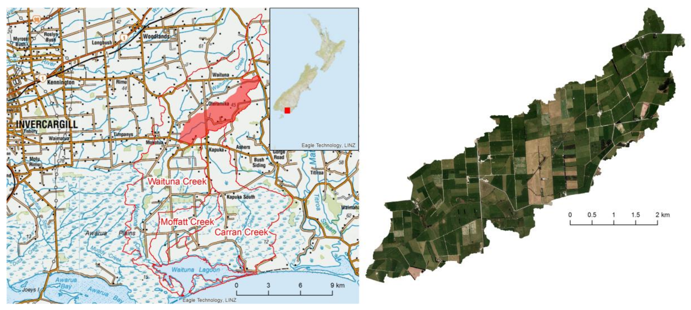
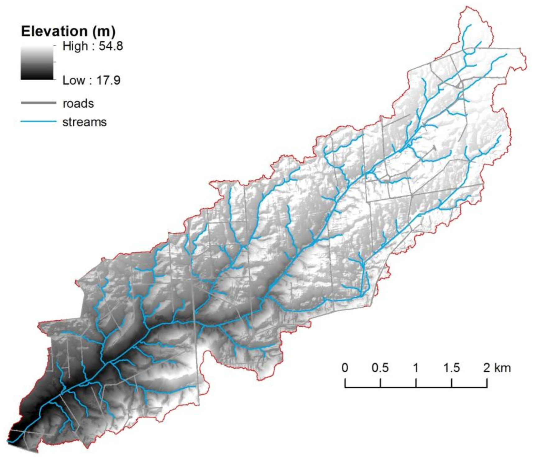
2.1. Study Area
2.2. Criteria for Wetland Creation or Restoration and Spatial Analysis
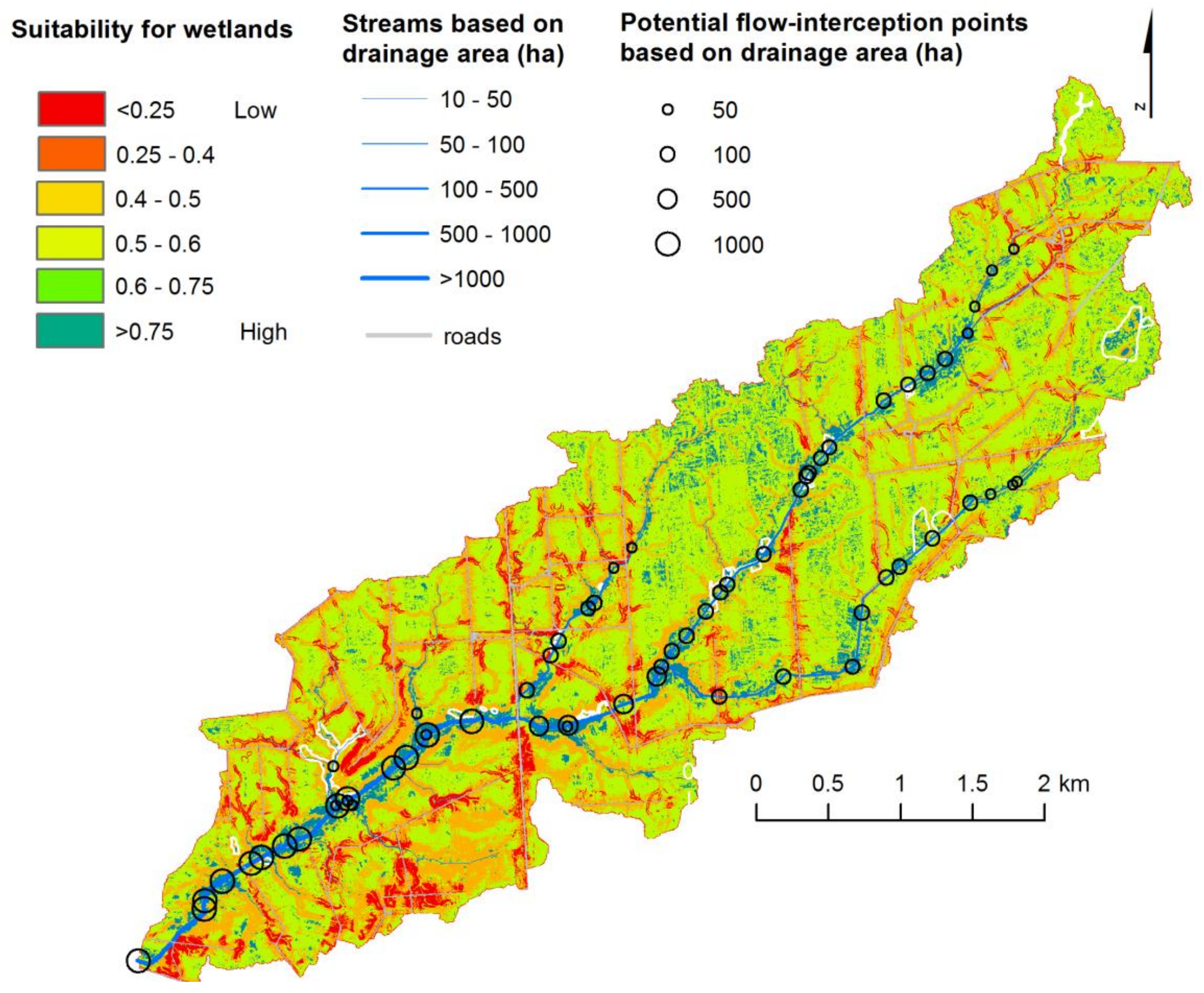
- Tile drain flows are the dominant hydrologic flow paths in the area, and the drains commonly follow natural drainage channels. Therefore, wetlands that are sited in these locations are also likely to intercept a high proportion of surface and subsurface run-off during large rainfall events [32]. Therefore, we only considered in-stream options in the current study (i.e., options in which the stream flows through or is closely adjacent to the wetland). In addition, in-stream wetlands require less investment than off-stream alternatives, and are a good option if the restoration budget is limited.
- The contributing area (i.e., the area that contributes water to the wetland) is an important criterion, since wetlands with a too-small contributing area may be ineffective for decreasing pollutant loads. (Here, we will focus on nitrogen pollution, but the same approach applies to most other pollutants.) The minimum area we chose for this study was 50 ha.
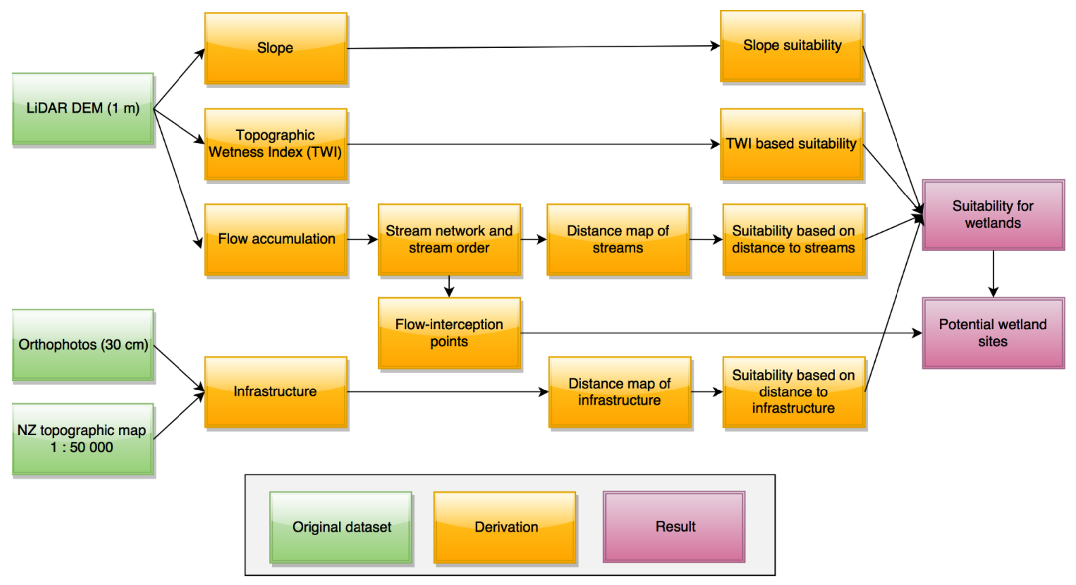
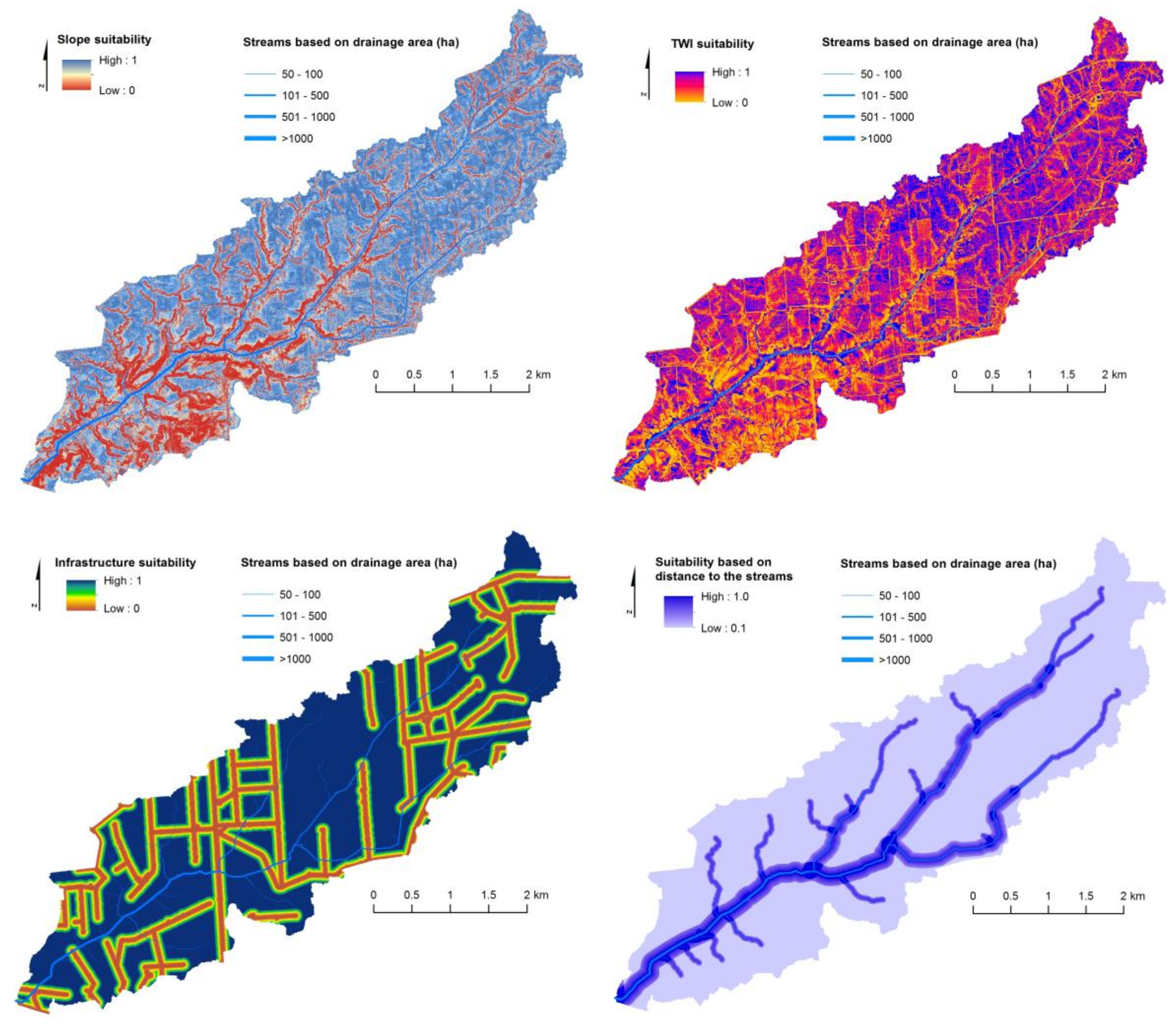
2.3. Suitability Modelling Approach
2.4. Delineation of Potential Wetlands
3. Results and Discussion
4. Conclusions
Acknowledgments
Author Contributions
Conflicts of Interest
References
- Kadlec, R.H. Constructed marshes for nitrate removal. Crit. Rev. Environ. Sci. Technol. 2012, 42, 934–1005. [Google Scholar] [CrossRef]
- Ausseil, A.G.E.; Dymond, J.R.; Shepherd, J.D. Rapid mapping and prioritisation of wetland sites in the Manawatu-Wanganui region, New Zealand. Environ. Manag. 2007, 39, 316–325. [Google Scholar] [CrossRef] [PubMed]
- Schleupner, C. GIS-based estimation of wetland conservation potentials in Europe. In Proceedings of the International Conference on Computational Science and Its Applications, Fukuoka, Japan, 23–26 March 2010; Taniar, D., Gervasi, O., Murgante, B., Pardede, E., Apduhan, B.O., Eds.; Springer: Berlin/Heidelberg, Germany, 2010; pp. 193–209, ISBN 978-3-642-12156-2. [Google Scholar]
- The Organisation for Economic Co-Operation and Development (OECD). Third Environmental Performance Review: New Zealand 2017; OECD: Paris, France, 2017. [Google Scholar]
- Matthew, C.; Horne, D.J.; Baker, R.D. Nitrogen loss: An emerging issue for the ongoing evolution of New Zealand dairy farming systems. Nutr. Cycl. Agroecosyst. 2010, 88, 289–298. [Google Scholar] [CrossRef]
- Moreno-Mateos, D.; Comin, F.A. Integrating objectives and scales for planning and implementing wetland restoration and creation in agricultural landscapes. J. Environ. Manag. 2010, 91, 2087–2095. [Google Scholar] [CrossRef] [PubMed]
- Dai, C.; Guo, H.C.; Tan, Q.; Ren, W. Development of a constructed wetland network for mitigating nonpoint source pollution through a GIS-based watershed-scale inexact optimization approach. Ecol. Eng. 2016, 96, 94–108. [Google Scholar] [CrossRef]
- Tomer, M.D.; Crumpton, W.G.; Bingner, R.L.; Kostel, J.A.; James, D.E. Estimating nitrate load reductions from placing constructed wetlands in a HUC-12 watershed using LiDAR data. Ecol. Eng. 2013, 56, 69–78. [Google Scholar] [CrossRef]
- Malczewski, J. GIS-based land-use suitability analysis: A critical overview. Prog. Plan. 2004, 62, 3–65. [Google Scholar] [CrossRef]
- Chen, J. GIS-based multi-criteria analysis for land use suitability assessment in City of Regina. Environ. Syst. Res. 2014, 3, 13. [Google Scholar] [CrossRef]
- Martinig, A.R. Habitat suitability modeling for mink passage activity: A cautionary tale. J. Wildl. Manag. 2017, 81, 1439–1448. [Google Scholar] [CrossRef]
- Guo, Y.L.; Wang, Q.; Yan, W.P.; Zhou, Q.; Shi, M.Q. Assessment of habitat suitability in the Upper Reaches of the Min River in China. J. Mt. Sci. 2015, 12, 737–746. [Google Scholar] [CrossRef]
- Akinci, H.; Özalp, A.Y.; Turgut, B. Agricultural land use suitability analysis using GIS and AHP technique. Comput. Electron. Agric. 2013, 97, 71–82. [Google Scholar] [CrossRef]
- Roy, P.S.; Murthy, M.S.R. Efficient Land Use Planning and Policies using Geospatial Inputs: An Indian Experience. In Land Use Policy; Denman, A.C., Penrod, O.M., Eds.; Nova Science Publishers: New York, NY, USA, 2009; pp. 31–72. ISBN 978-1-60741-435-3. [Google Scholar]
- Collins, M.G.; Steiner, F.R.; Rushman, M.J. Land-use suitability analysis in the United States: Historical development and promising technological achievements. Environ. Manag. 2001, 28, 611–621. [Google Scholar] [CrossRef] [PubMed]
- White, D.; Fennessy, S. Modeling the suitability of wetland restoration potential at the watershed scale. Ecol. Eng. 2005, 24, 359–377. [Google Scholar] [CrossRef]
- Babbar-Sebens, M.; Barr, R.C.; Tedesco, L.P.; Anderson, M. Spatial identification and optimization of upland wetlands in agricultural watersheds. Ecol. Eng. 2013, 52, 130–142. [Google Scholar] [CrossRef]
- Berthier, L.; Guzmova, L.; Laroche, B.; Lehmann, S.; Squivident, H.; Martin, M.; Chenu, J.-P.; Thiry, E.; Lemercier, B.; Bardy, M.; et al. Spatial prediction of potential wetlands at the French national scale based on hydroecoregions stratification and inference modelling. In Proceedings of the EGU General Assembly 2014, Vienna, Austria, 27 April–2 May 2014. [Google Scholar]
- Odgaard, M.V.; Turner, K.G.; Bøcher, P.K.; Svenning, J.C.; Dalgaard, T. A multi-criteria, ecosystem-service value method used to assess catchment suitability for potential wetland reconstruction in Denmark. Ecol. Indic. 2017, 77, 151–165. [Google Scholar] [CrossRef]
- Tiner, R.W.; Lang, M.W.; Klemas, V.V. Remote Sensing of Wetlands: Applications and Advances; CRC Press: Boca Raton, FL, USA, 2014; Volume GE-21, ISBN 978-1-4822-3735-1. [Google Scholar]
- Ozesmi, S.L.; Bauer, M.E. Satellite remote sensing of wetlands. Wetl. Ecol. Manag. 2002, 10, 381–402. [Google Scholar] [CrossRef]
- Merot, P.; Hubert-Moy, L.; Gascuel-Odoux, C.; Clement, B.; Durand, P.; Baudry, J.; Thenail, C. A method for improving the management of controversial wetland. Environ. Manag. 2006, 37, 258–270. [Google Scholar] [CrossRef] [PubMed]
- McKergow, L.A.; Gallant, J.C.; Dowling, T.I. Modelling wetland extent using terrain indices, Lake Taupo, NZ. In Proceedings of the International Congress on Modelling and Simulation: LAND, Water and Environmental Management: Integrated Systems for Sustainability, Christchurch, New Zealand, 10–13 December 2007; Kulasiri, D., Oxley, L., Eds.; Modelling and Simulation Society of Australia and New Zealand. 2007; pp. 1335–1341. [Google Scholar]
- Murgoitio, J.; Shrestha, R.; Glenn, N.; Spaete, L. Airborne LiDAR and terrestrial laser scanning derived vegetation obstruction factors for visibility models. Trans. GIS 2014, 18, 147–160. [Google Scholar] [CrossRef]
- Waz, A.; Creed, I.F. Automated Techniques to Identify Lost and Restorable Wetlands in the Prairie Pothole Region. Wetlands 2017, 37, 1079–1091. [Google Scholar] [CrossRef]
- Holmes, D.; McEvoy, J.; Dixon, J.; Payne, S. A Geospatial Approach for Identifying and Exploring Potential Natural Water Storage Sites. Water 2017, 9, 585. [Google Scholar] [CrossRef]
- Jones, C.N.; Evenson, G.R.; McLaughlin, D.L.; Vanderhoof, M.K.; Lang, M.W.; McCarty, G.W.; Golden, H.E.; Lane, C.R.; Alexander, L.C. Estimating restorable wetland water storage at landscape scales. Hydrol. Process. 2018, 32, 305–313. [Google Scholar] [CrossRef]
- Lang, M.; McDonough, O.; McCarty, G.; Oesterling, R.; Wilen, B. Enhanced detection of wetland-stream connectivity using lidar. Wetlands 2012, 32, 461–473. [Google Scholar] [CrossRef]
- Wu, Q.; Lane, C.R. Delineating wetland catchments and modeling hydrologic connectivity using lidar data and aerial imagery. Hydrol. Earth Syst. Sci. 2017, 21, 3579–3595. [Google Scholar] [CrossRef]
- Nie, S.; Wang, C.; Xi, X.; Luo, S.; Li, S.; Tian, J. Estimating the height of wetland vegetation using airborne discrete-return LiDAR data. Optik (Stuttg) 2018, 154, 267–274. [Google Scholar] [CrossRef]
- Meneses, N.C.; Baier, S.; Geist, J.; Schneider, T. Evaluation of green-LiDAR data for mapping extent, density and height of aquatic reed beds at Lake Chiemsee, Bavaria-Germany. Remote Sens. 2017, 9, 1308. [Google Scholar] [CrossRef]
- Tanner, C.; Sukias, J.; Burger, D. Realising the value of remnant wetlands as farm attenuation assets. In Annual Fertiliser and Lime Research Centre Workshop, Moving Farm Systems to Improved Nutrient Attenuation; Currie, L.D., Burkitt, L.L., Eds.; Fertilizer and Lime Research Centre: Massey University, Palmerston North, New Zealand, 2015. [Google Scholar]
- Kadlec, R.H.; Wallace, S.D. Treatment Wetlands, 2nd ed.; CRC Press: Boca Raton, FL, USA, 2009; ISBN 9781566705264. [Google Scholar]
- U.S. Environmental Protection Agency (EPA). Manual: Constructed Wetlands Treatment of Municipal Wastewaters; EPA/625/R-99/010; U.S. Environmental Protection Agency: Washington, DC, USA, 2000; 166p.
- Tournebize, J.; Chaumont, C.; Mander, Ü. Implications for constructed wetlands to mitigate nitrate and pesticide pollution in agricultural drained watersheds. Ecol. Eng. 2017, 103, 415–425. [Google Scholar] [CrossRef]
- ESRI ArcGIS Desktop: Release 10.2, Environmental Systems Research Institute: Redlands, CA, USA, 2013.
- Jenson, S.K.; Domingue, J.O. Extracting topographic structure from digital elevation data for geographic information system analysis. Photogramm. Eng. Remote Sens. 1988, 54, 1593–1600. [Google Scholar]
- Strahler, A.N. Quantitative analysis of watershed geomorphology. Eos Trans. Am. Geophys. Union 1957, 38, 913–920. [Google Scholar] [CrossRef]
- Beven, K.J.; Kirkby, M.J. A physically based, variable contributing area model of basin hydrology. Hydrol. Sci. Bull. 1979, 24, 43–69. [Google Scholar] [CrossRef]
- Infascelli, R.; Faugno, S.; Pindozzi, S.; Boccia, L.; Merot, P. Testing Different Topographic Indexes to Predict Wetlands Distribution. Procedia Environ. Sci. 2013, 19, 733–746. [Google Scholar] [CrossRef]
- Conrad, O.; Bechtel, B.; Bock, M.; Dietrich, H.; Fischer, E.; Gerlitz, L.; Wehberg, J.; Wichmann, V.; Böhner, J. System for Automated Geoscientific Analyses (SAGA) v. 2.1.4. Geosci. Model Dev. 2015, 8, 1991–2007. [Google Scholar] [CrossRef]
- LINZ Southland & Central Otago 0.4 m Rural Aerial Photos (2013-14). Available online: Https://data.linz.govt.nz/layer/2344-southland-central-otago-04m-rural-aerial-photos-2013-14/ (accessed on 15 January 2018).
- Galletti, C.S.; Myint, S.W. Land-use mapping in a mixed urban-agricultural arid landscape using object-based image analysis: A case study from Maricopa, Arizona. Remote Sens. 2014, 6, 6089–6110. [Google Scholar] [CrossRef] [Green Version]
- LINZ NZ Parcels. Available online: Https://data.linz.govt.nz/layer/51571-nz-parcels/ (accessed on 29 January 2018).
- Beinat, E. Value Functions for Environmental Management; Springer: Dordrecht, The Netherlands, 1997; Volume 1, ISBN 978-94-015-8885-0. [Google Scholar]
- Carver, S.J. Integrating multi-criteria evaluation with geographical information systems. Int. J. Geogr. Inf. Syst. 1991, 5, 321–339. [Google Scholar] [CrossRef]
- Eastman, J.R.; Jin, W.; Kyem, P.A.K.; Toledano, J. Raster Procedures for multi-criteria/multi-objective decisions. Photogramm. Eng. Remote Sens. 1995, 61, 539–547. [Google Scholar]
- Cheng, F.Y.; Basu, N.B. Biogeochemical hotspots: Role of small water bodies in landscape nutrient processing. Water Resour. Res. 2017, 53, 5038–5056. [Google Scholar] [CrossRef]
- Bengtson, M.L.; Padmanabhan, G. A Review of Models for Investigating the Influence of Wetlands on Flooding; North Dakota Water Resources Research Institute, North Dakota State University: Fargo, ND, USA, 1999. [Google Scholar]
- Van der Valk, A.G.; Jolly, R.W. Recommendations for research to develop guidelines for the use of wetlands to control rural nonpoint source pollution. Ecol. Eng. 1992, 1, 115–134. [Google Scholar] [CrossRef]
- Peterson, B.J. Control of Nitrogen Export from Watersheds by Headwater Streams. Science 2001, 292, 86–90. [Google Scholar] [CrossRef] [PubMed]
- Tanner, C.; Kadlec, R. Influence of hydrological regime on wetland attenuation of diffuse agricultural nitrate losses. Ecol. Eng. 2013, 56, 79–88. [Google Scholar] [CrossRef]
- Tournebize, J.; Gramaglia, C.; Birmant, F.; Bouarfa, S.; Chaumont, C.; Vincent, B. Co-design of constructed wetlands to mitigate pesticide pollution in a drained catch-Basin: A solution to improve groundwater quality. Irrig. Drain. 2012, 61, 75–86. [Google Scholar] [CrossRef]
- Kusler, J. Common Questions: Wetland Definition, Delineation, and Mapping; Association of State Wetland Managers Inc.: New York, NY, USA, 2000. [Google Scholar]
- Grealish, G. New Zealand Soil Mapping Protocols and Guidelines; Landcare Research, Massey University: Palmerston North, New Zealand, 2017. [Google Scholar]
- Heywood, I.; Oliver, J.; Tomlinson, S. Building an exploratory multi-criteria modelling environment for spatial decision support. Innov. GIS 1995, 2, 127–136. [Google Scholar]
- Romano, G.; Dal Sasso, P.; Trisorio Liuzzi, G.; Gentile, F. Multi-criteria decision analysis for land suitability mapping in a rural area of Southern Italy. Land Use Policy 2015, 48, 131–143. [Google Scholar] [CrossRef]
- Gleason, R.A.; Tangen, B.A.; Laubhan, M.K.; Kermes, K.E.; Euliss, N.H., Jr. Estimating Water Storage Capacity of Existing and Potentially Restorable Wetland Depressions in a Subbasin of the Red River of the North; USGS Northern Prairie Wildlife Research Center: Reston, VA, USA, 2007.
- Fernandez-Nunez, M.; Burningham, H.; Ojeda Zujar, J. Improving accuracy of LiDAR-derived digital terrain models for saltmarsh management. J. Coast. Conserv. 2017, 21, 209–222. [Google Scholar] [CrossRef]


| Wetland ID | Contributing Area (ha) | Wetland Area (ha) | Proportion Within the Catchment (%) | Average Depth (m) | No. of Cadastral Parcels | Water Storage Capacity (103 m3) |
|---|---|---|---|---|---|---|
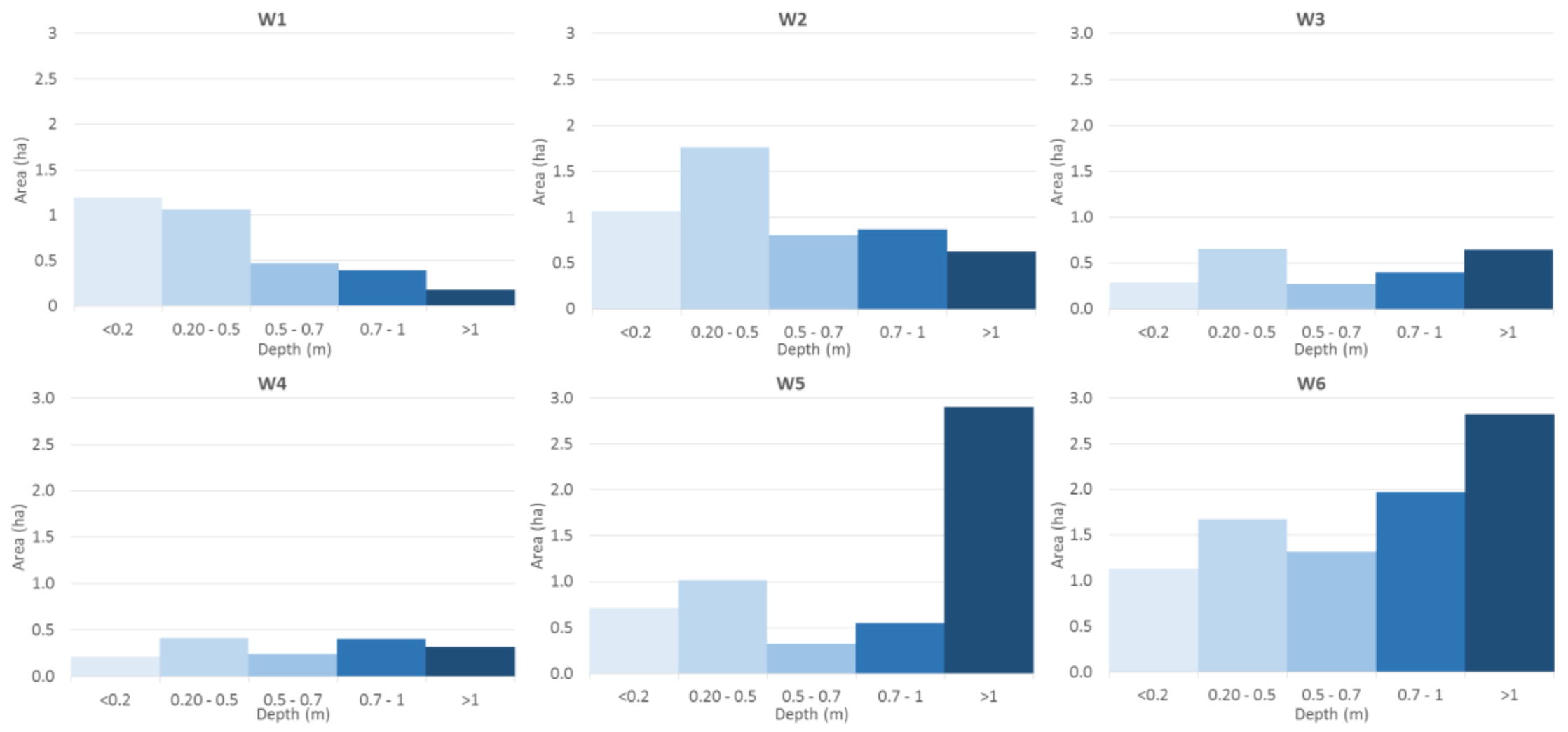
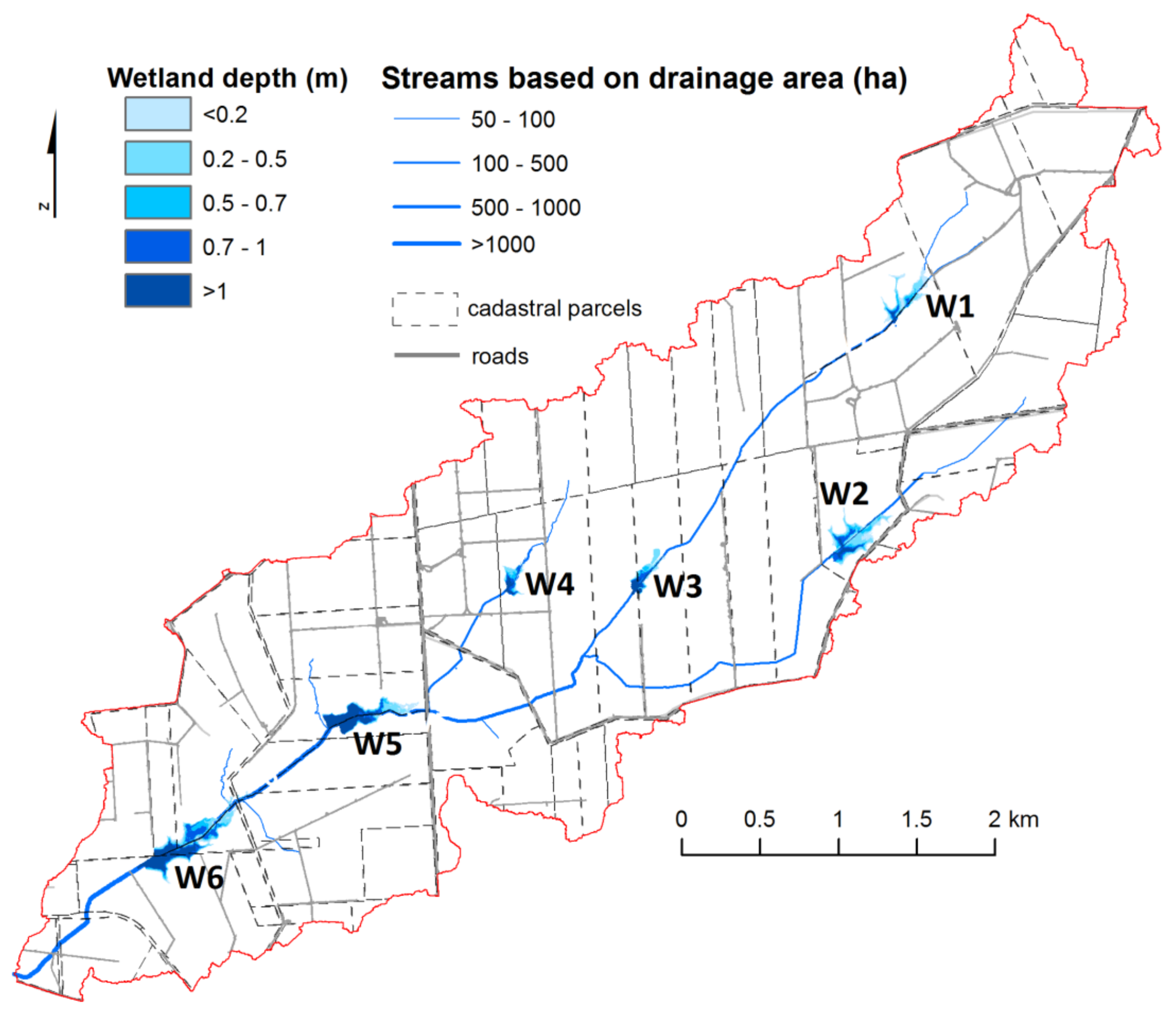
| W1 | 175.3 | 3.3 | 1.9 | 0.4 | 1 | 13.0 |
| W2 | 155.7 | 5.2 | 3.3 | 0.5 | 1 | 27.5 |
| W3 | 455.4 | 2.4 | 0.5 | 0.7 | 2 | 17.8 |
| W4 | 133.8 | 1.6 | 1.2 | 0.7 | 1 | 11.1 |
| W5 | 1115.1 | 5.5 | 0.5 | 1.0 | 2 | 61.3 |
| W6 | 1484.8 | 8.9 | 0.6 | 0.8 | 5 | 73.2 |
| Total | 1584.5 | 26.9 | 1.7 | 203.9 |
© 2018 by the authors. Licensee MDPI, Basel, Switzerland. This article is an open access article distributed under the terms and conditions of the Creative Commons Attribution (CC BY) license (http://creativecommons.org/licenses/by/4.0/).
Share and Cite
Uuemaa, E.; Hughes, A.O.; Tanner, C.C. Identifying Feasible Locations for Wetland Creation or Restoration in Catchments by Suitability Modelling Using Light Detection and Ranging (LiDAR) Digital Elevation Model (DEM). Water 2018, 10, 464. https://doi.org/10.3390/w10040464
Uuemaa E, Hughes AO, Tanner CC. Identifying Feasible Locations for Wetland Creation or Restoration in Catchments by Suitability Modelling Using Light Detection and Ranging (LiDAR) Digital Elevation Model (DEM). Water. 2018; 10(4):464. https://doi.org/10.3390/w10040464
Chicago/Turabian StyleUuemaa, Evelyn, Andrew O. Hughes, and Chris C. Tanner. 2018. "Identifying Feasible Locations for Wetland Creation or Restoration in Catchments by Suitability Modelling Using Light Detection and Ranging (LiDAR) Digital Elevation Model (DEM)" Water 10, no. 4: 464. https://doi.org/10.3390/w10040464