Predicting Sedimentation in Urban Sewer Conduits


1
Department of Civil and Environmental Engineering, Hanbat National University, Daejeon 34158, Korea
2
Department of Mechanical Engineering, Hanbat National University, Daejeon 34158, Korea
3
Research Center for Disaster Prevention Science and Technology, Korea University, Seoul 02841, Korea
*
Author to whom correspondence should be addressed.
Water 2018, 10(4), 462; https://doi.org/10.3390/w10040462
Submission received: 28 February 2018
/
Revised: 31 March 2018
/
Accepted: 7 April 2018
/
Published: 11 April 2018
Abstract
:Sedimentation commonly occurs in urban drainage systems, disrupts flow, and is one of the major causes of inundation. The complicated phenomena that alter the cross-section of sewer conduits include transportation, precipitation, and sedimentation, and need to be analyzed for the proper design and efficient maintenance of urban drainage systems. In this study, the discharge capacity of urban drainage systems is simulated and analyzed by considering the pattern of flow of sediments in sewer conduits through a numerical analysis model. The sites of the highest and lowest accumulation of soil were examined as sedimentation occurred, as was discharge due to accumulation in sewer conduits. The purpose of this study is the examination of mathematical models for two-phase fluid flow analysis and the prediction of sedimentation in urban sewer conduits. An expression for the height of the sedimentation was obtained to assess the discharge capacity of urban drainage systems, and a model to predict accumulation in sewer conduits was developed using non-dimensional variables for inlet velocity, inlet particle volume fraction, and particle size. When subjected to linear regression analysis, the model yielded a high correlation coefficient (R2) of 0.899. This satisfied the aims of this study, to obtain a higher discharge capacity and a plan for the design of urban drainage systems.
1. Introduction
A large amount of research has been conducted on sediment disasters in urban drainage systems. In addition to an analysis of the characteristics of soil erosion in the watershed, a description of the internal phenomena has emerged as important. Causes of urban inundation have been examined from various viewpoints, and the volume of sedimentation inside sewer conduits has been highlighted as a major problem. Soil accumulates in the drainage conduits and frequently blocks them, thus leading to flooding in urban areas. It is essential to prevent sediment deposition in sewers by means of proper design schemes, i.e., through enhanced design of sewer networks by considering sediment transport.
Researchers have studied the phenomenon of sediment transport by considering mainly open-channel states, such as in rivers [1,2,3]. A river can be used for sediment deposition and transport analysis based on a variety of observed data. It is possible to estimate the range of influence by using hydraulic parameters. The relevant studies have primarily used data collection and analysis based on the river bed to calculate the rate of sedimentation. However, it is challenging to obtain data on sediment transport and sedimentation in urban drainage systems because sediment flow in sewer conduits is very unstable [4,5,6].
The results of the empirical process are hydraulic characteristics of a single fluid. It is impossible to model a phenomenon when a complex process occurs at the same time, and thus two-phase flow must be considered [7,8,9,10,11,12]. Moreover, mixing occurs inside conduits when soil enters them [13,14,15,16].
Many studies were suggested for the sediment transportation. The Hydrass flushing gate and field validation of flush propagation modelling were suggested for the flush cleaning of sewers [17,18]; a cleaning operation including installation of a sediment trap or a flushing sump/chamber in front of outlet [19]. The 1D De Saint Venant-Exner equations were applied to numerical modelling [20]. However, there is no application of two-phase flow for the sediment transportation in urban sewer conduits.
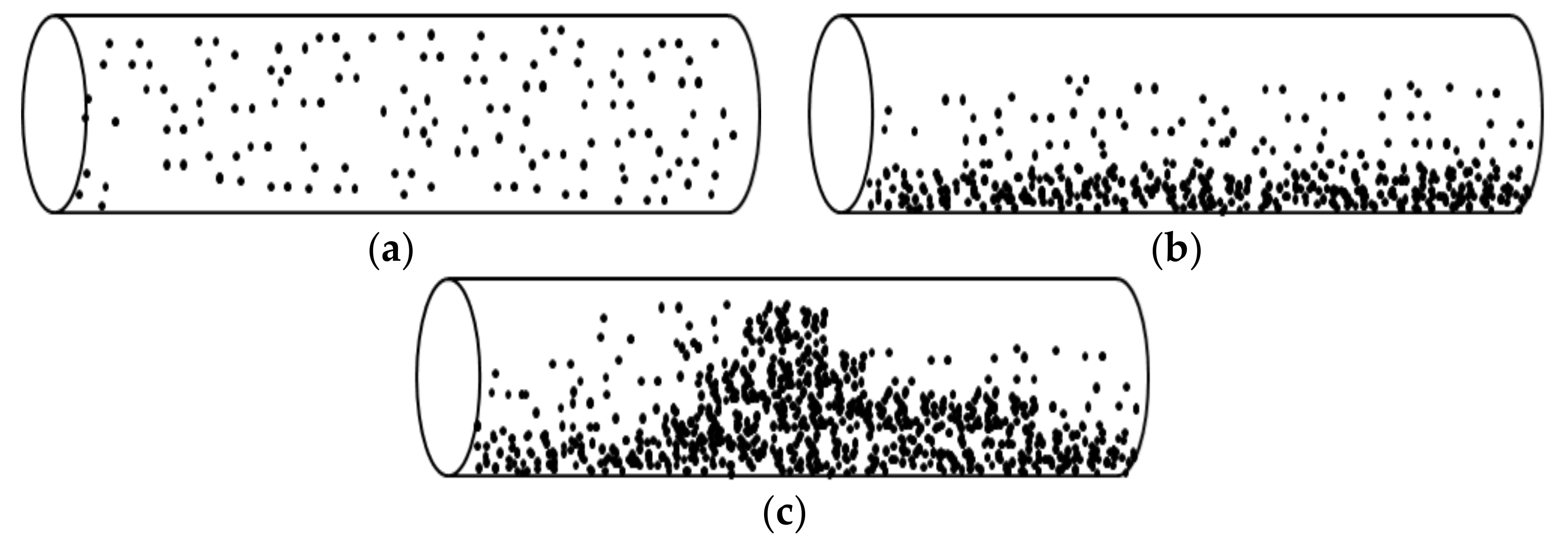
Two-phase flow is an example of multiphase flow and can occur in various forms. The results of empirical processes according to the hydrodynamic properties of single-phase fluids are different from those of phenomena involving a two-phase flow composed of soils and fluids. The two-phase flow can be classified as shown in Figure 1: homogeneous flow, where soil particles move uniformly throughout the pipe (Figure 1a); separated flow or dune flow, where particles with high density settle at the bottom and flow (Figure 1b); and slug flow, where large bubbles are created and move (Figure 1c). The flow of mixtures of soil and water follows a two-phase pattern, where homogeneous mixtures are as shown in Figure 1a, and soil particles with high density settle at the bottom and move as in Figure 1b. This study reports the modeling of two-phase flow patterns as shown in Figure 1b.
In this study, an ANSYS-Fluent numerical model, a solver of computational fluid dynamics (CFD) models, was applied for analysis. It is among the most widely used commercial CFD solvers in practical and academic research in mechanical and industrial engineering [21,22,23].
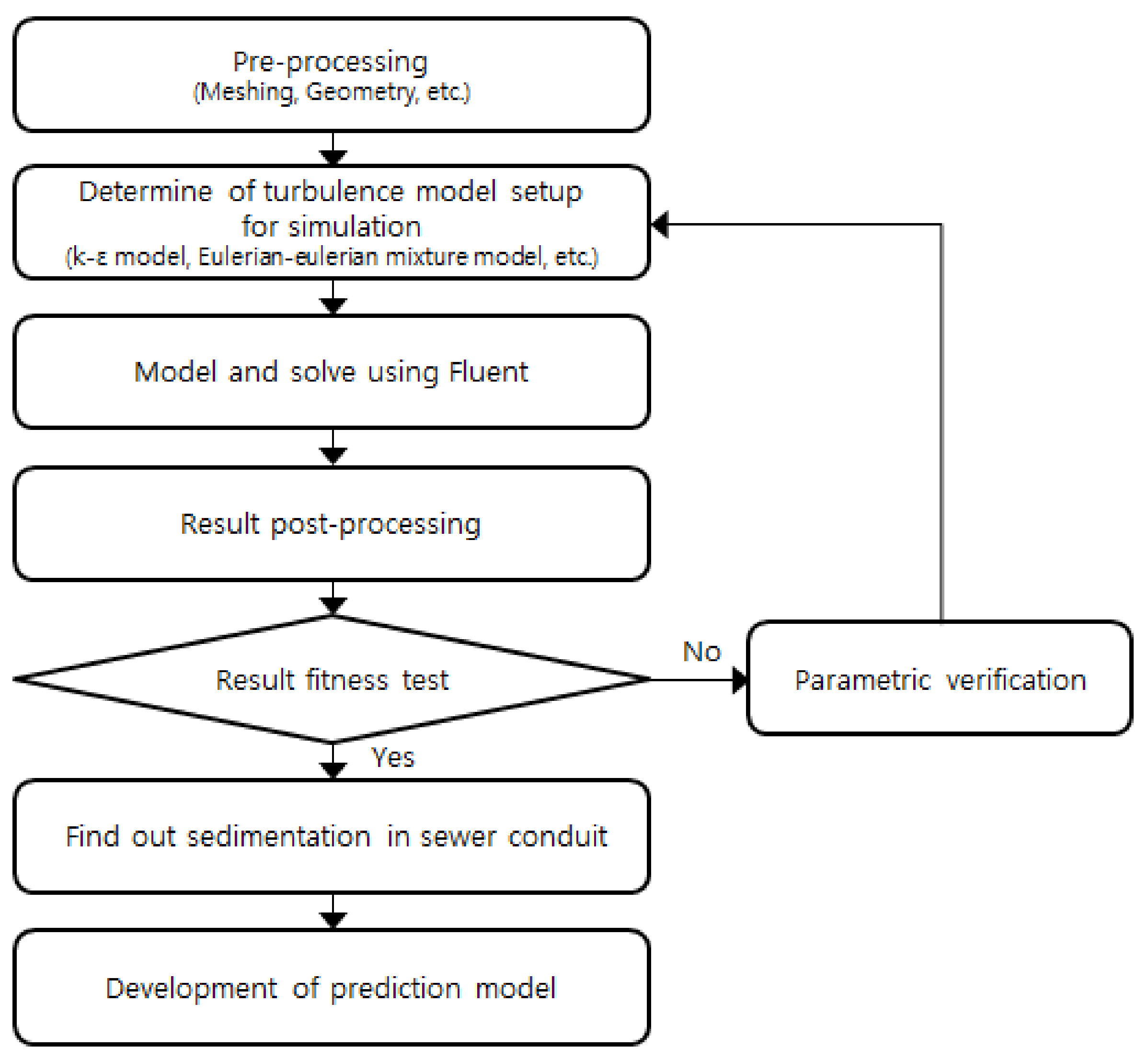
In the process of validation, various changes measured in an experiment involving a pipe performed by Nabil et al. [7] was simulated. The effects of inlet velocity, the size of soil particles, the volume fraction of soil, the flow characteristics of the water mixture, and soil distribution inside the conduits were numerically investigated by using a two-phase mixture model. The characteristics of soil and water slurry were numerically investigated in pipeline flow. Conduits with horizontal locations were used in the simulation. Based on the results, the authors develop a sedimentation height formula to assess the discharge capacity of an urban drainage system by considering sediments in conduits. A flow chart of the analysis procedure is shown Figure 2.
2. Methodologies
2.1. Overview
Soil transfer inside conduits is complex to model because of an insufficient amount of observational or empirical data. Moreover, the physical complexity of sediment transport, settling, sedimentation, and erosion in conduits must be considered. Parameters such as the critical flow rate, shear stress, particle properties, and hydraulic parameters in conduits must also be considered. Fluid flow within conduits cannot be characterized as involving a single fluid; it is modeled as two-phase flow with soil. Therefore, it is necessary to consider interactions using both fluid statics and dynamics. The purpose of numerical modeling is the examination of mathematical models for two-phase fluid flow analysis.
In all problems involving CFD analysis, it is essential to determine the initial and boundary conditions. It is important for the user to design a model to analyze and implement numerical models suitable for this. The solutions are obtained through proper operating procedures. In unsteady and turbulent flows, all variables used for analysis have different values in the overall flow areas from the initial values. Those (initial values) could be represented as the important variables [20]. There are several assumptions for the modelling. The assumptions consist of:
- The two-phase flow of a single sewer conduit was simulated
- The pipe channel instead of open channel was used for simulations
- The mixture and turbulent flows was assumed
- The same diameter of particle flows to a single sewer conduit.
2.2. Governing Equations
To analyze the inflow rate of fluid containing soil particles, it is necessary to analyze the flow of two-phase fluids. Boris et al. used the eulerian-eulerian CFD model for the sedimentation of spherical particle concentrations [24,25]. Lixing analyzed the two-phase turbulence model in eulerian-eulerian simulations and Zhen et al. suggested a multi-dimensional eulerian two-phase model for sediment transport [26,27]. Many studies used the eulerian-eulerian model for the particle transportation and this study uses an eulerian-eulerian model. The two-phases are handled and analyzed as continua that are preserved, and the volume occupied by one cannot be occupied by the other. The concept of volume fractions is hence introduced. These volume fractions are assumed as continuous functions of space and time and their sum is always constant. The governing equations for all phases can be obtained using the conservation equation for each. The modeling methods of two-phase flows, such as a mixture of soil and fluids, using numerical analysis can be largely classified into an eulerian method that assumes that the soil particles are a continuum, like a fluid, and a Lagrange method that applies Newton’s laws of force and motion to the soil particles. The methods of analyzing soil particles as a continuum can be further classified into a single-fluid model that applies continuity equations, momentum equations, and particle component conservation equations by handling a mixture of soil and water as a fluid, and a two-phase separation model that applies the laws of conservation to the soil particles and the fluid, respectively.
ANSYS-Fluent calls the above two models a mixture model [28], and an eulerian–eulerian model, respectively, and both have yielded very similar results in previous studies [7,9,10]. The same result of this study and previous studies is the sedimentation of a sewer conduit in the process of transport modelling. This study uses the mixture model with a high computational efficiency. Although the mixture model handles the mixture as a single fluid, all component equations for the soil particles, gravitation, and interactions between fluids and soil particles, and within the soil particles can be applied to the momentum equations. Its computation is relatively easy, and thus is widely used to model a mixture of soil particles and fluids. In general, the analysis of flow characteristics using a slurry composed of soil particles and fluids involves the use of an eulerian–eulerian two-phase flow model. The model is used to analyze the flow of soil particles as the motion of fluids.
The eulerian–eulerian method obtains a flow rate field and a soil particle distribution field by solving the continuity Equations (1) and (2), the momentum Equations (3) and (4), and the standard k–ε turbulence equation. In the k–ε turbulence model [29], the correlation term in the flow velocity variations is represented in a Reynolds’ stress term by averaging the values of the Nävier–Stokes equation over time under the assumption that a turbulent flow velocity varying in time can be divided into a time average flow velocity and a variant flow velocity. Each equation follows the laws of conservation of mass and momentum, suitable for analyzing the effect of turbulence on each boundary surface in an arbitrary inspection volume set to analyze the flow in a conduit of urban drainage systems. Equation (1) is a continuity equation representing the transfer of momenta for pressure, viscosity, turbulent stress energy, the transfer of volumetric fractions, and densities per time of each phase based on the flow velocity components of momentum in Equation (2).
In particular, the momentum equation should reflect interactions between soil particles and fluids; thus, Fc and Fd in Equations (3) and (4) represent the drag force and the lift force due to the interactions between the fluids and soil particles, respectively, for which commercial programs provide various models as options. This study applied the Syamlal–O’Brien model [30] as a particle viscosity and pressure model [31,32,33,34], and it was also used as a drag force model. The continuity equations are shown as Equations (1) and (2), and the momentum equations as Equations (3) and (4):
where u is fluid velocity, is the density of the fluid, is the volume fraction of each phase, is the vector differential operator, p is pressure, g is the gravitational constant, and µ is dynamic viscosity.
2.3. Model for Analysis
To analyze the effect of turbulence inside the conduits into which particles of fluid and soil are introduced, it is necessary to consider the turbulence model. When a fluid moves continuously, a laminar flow appears finally as shear force owing to the laminar viscous force between neighboring fluids as a driving force. However, if flow velocity increases for the shear stress to become very strong, the transfer by the viscous force cannot bear this, such that the shear force is broken by very small turbulent eddies that transfer the shear force to inside the fluid. As flow velocity increases further, the size of the turbulent eddies decreases and the behavior of the fluids varies significantly depending on changes in time. The temporal average values of turbulent flow vary in a constant form and the fluctuation values have short temporal periods.
To analyze the flow composed of soil particles and fluids, it is necessary to analyze two-phase fluids. This study used the eulerian–eulerian model and the k–ε model to analyze the continuity equations and turbulent motion. k represents physically the turbulent kinematic energy, defined as turbulent perturbation velocity, which in turn is defined as turbulent dissipation rate. The k–ε model is an eddy viscosity model, from which μt can be obtained through k and ε in Equation (5):
Cu is a model constant that takes a value of 0.09 in general [24]. In local areas, depending on the generation of sedimentation in conduits, turbulent stress can be modeled by computing k and ε using two transport equations, such as Equations (6)–(8):
In these equations, represents the generated turbulent kinetic energy owing to the mean velocity gradients, is the generated turbulent kinetic energy due to buoyancy, represents the contribution of the fluctuating dilatation in compressible turbulence to the overall dissipation rate, and are constants, and are the turbulent Prandtl numbers for k and ε, respectively, and and are user-defined source terms [35].
Each coefficient in Equations (5)–(8) uses the following values in the standard k–ε model such as Table 1:
, , , and are unknown. The values of these constants are determined by numerous iterations involving data fitting for a wide range of turbulent flows. It finally becomes possible to accept them as below [36].
In the k–ε model, under the assumption that turbulent flow velocity varying in time can be divided into temporal average flow velocity and fluctuation flow velocity, the Nävier–Stokes equation is a time-averaged equation to indicate the correlation term in flow velocity fluctuations under a Reynolds’ stress term.
2.4. Boundary Conditions
The boundary conditions considered in this study were diverse and related to the inlets, outlets, and walls in general. The inlets are areas in which all information related to the flows is known, for which the user can define flow velocity, pressure, characteristic length, turbulence strength, and temperature. The outlets can be used when all directions of flow in the outlets are known, for which information concerning the flows is unnecessary.
This study assumed that the inflow conditions did not change over time or were due to other features. Because of this, simulations representing the phenomenon could be created by assuming a diversity of outflows. The computation time was also reduced to enable recursive computations. The boundaries for the sections used for analysis were the walls, and flow inlets and outlets, of which the former were constrained by a no-slip condition. The inlet of the conduit had the condition whereby the fluids and soil particles compulsively flowed in, and the outlet had the same conditions as a natural outlet with outflow characteristics. Because the shapes of the inlets and outlets were not complex, the inlets were used as flow boundary conditions and the outlets as differential pressure boundary conditions to set an outflow relationship. The following Table 2 summarizes all of the analysis conditions.
2.5. Validation of Model
To verify the analysis, the results were compared with experimental results in [7]. The facilities used for the water–soil slurry flow experiment primarily consisted of a sump tank, a centrifugal pump, piping, and a test part. The test part was a U-shaped pipe of length 10.55 m and inner diameter 150 mm. The volume distribution in the slurry flow was measured using a radiation density meter and flow velocity distribution was measured through the impedance between electrodes installed on the floor of the piping. The impedance between the electrodes represents the electric field formed by them as changed by the slurry. The slurry flow rate was measured using an electronic flow rate meter. As an experimental method, 0.2–2.0 mm of soil particles and water were adjusted according to the given volume fractions in a sump tank, circulated by a centrifugal pump through a test part and a visual part in turn, and were returned to the sump tank. Various measurements were performed during this time.
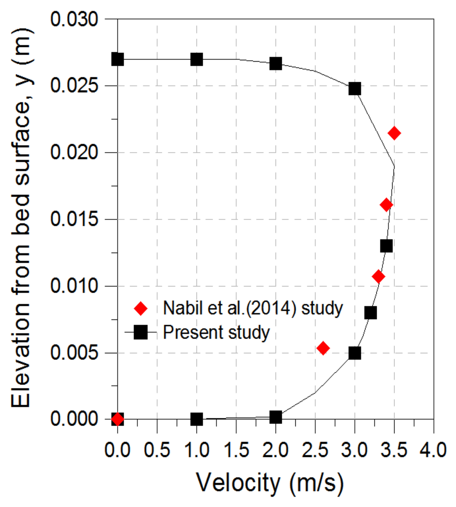
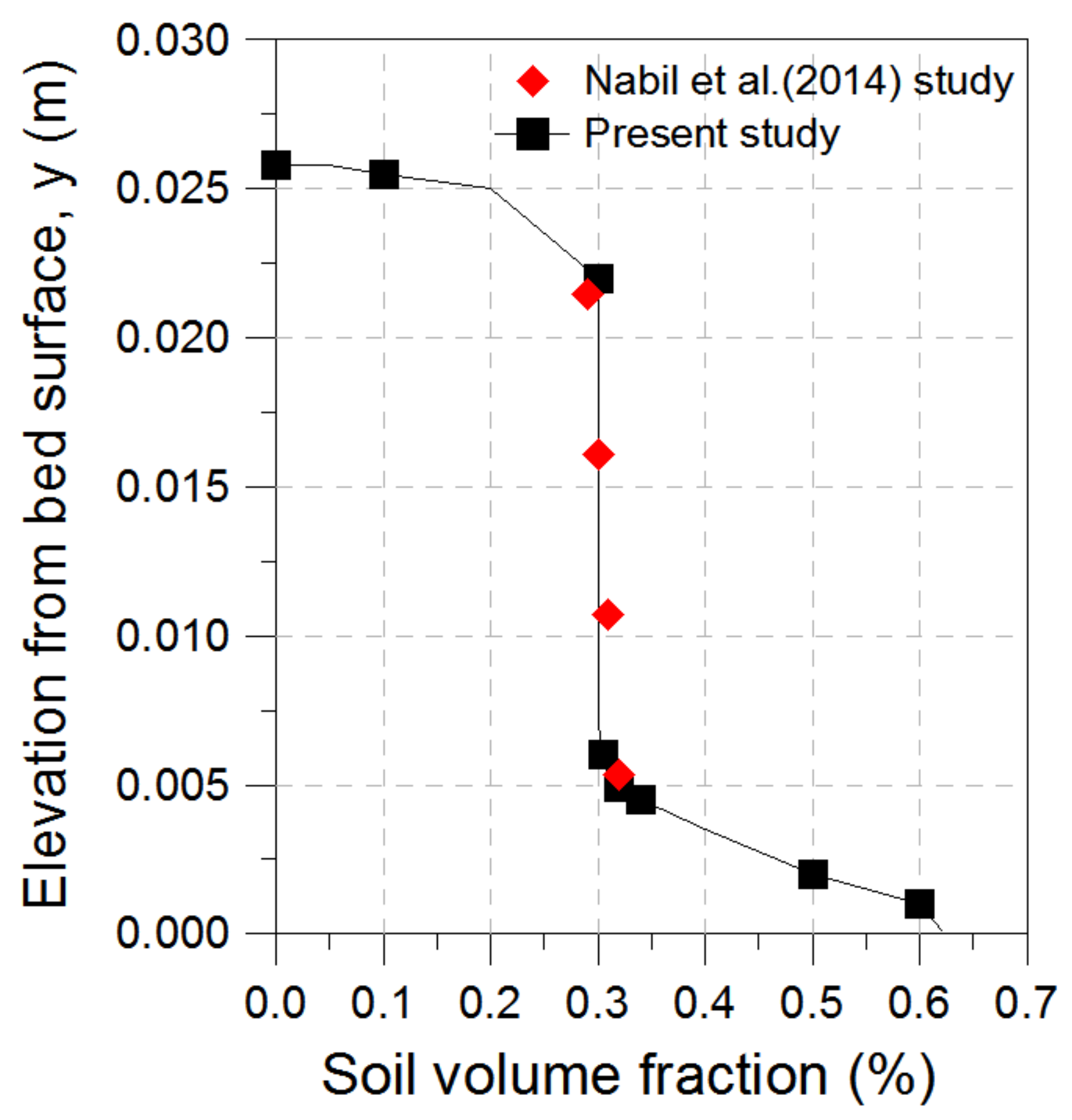
Table 3 shows conditions for the verification of the analysis. Figure 3 and Figure 4 show the volume distribution of the soil particles and the flow velocity distribution of the mixtures in slurry, respectively. The former in the pipe, at relatively fast flow velocity, was slightly greater at the bottom of the conduit but was uniform on the whole at 30%, similarly to the distribution at the inlet, and the flow velocity distribution of the mixtures was higher at the top of the pipe than the bottom owing to the partial deposition of soil at the bottom. The results of the flow phenomena yielded predictions similar to the experiment results as shown in Figure 3 and Figure 4.
3. Slurry Flow in Sewer Conduits
The authors analyzed 63 simulation conditions based on the conditions listed in Table 4. The computation was carried out up to a total of 500 s by applying a computation time interval ∆t = 1 s, where the computation was set to repeat 10 times the internal computations (step length factor). Using very small values in repetitions of the computation could have led to a termination of the analysis during particle transport and deposition, but interval used in this study was large enough to avoid this outcome. It was thus confirmed that the results did not change after a certain time in the analysis.
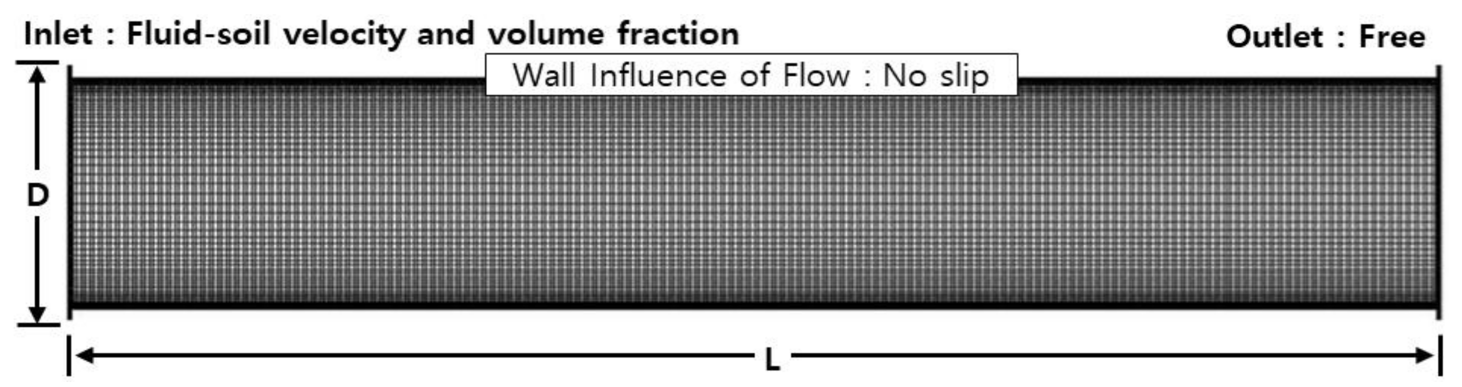
To simulate the deposition of soil flowing through a conduit, short conduits were used. For numerical simulations, a CFD analysis was carried out for incoming mixtures by considering the shape of drainage conduits and the type of connection of specific facilities. A total of 140,000 rectangular meshes, each 0.6 m in diameter and 10 m long, were used; no symmetrical boundaries were applied but the shape of the entire conduit was represented. Triangular meshes were used to analyze the drainage conduits, whereas rectangular meshes are suitable for analyzing structures with complex shapes and are easy to create.
Figure 5 shows the area of numerical analysis and the mesh used for the drainage conduits. The meshes were generated using an internal mesh creation model of the ANSYS-WORKBENCH [37]. The soil passing through the drainage conduit had particles of different sizes, and their distribution needed to be considered for modeling. However, this study assumed uniform incoming particle size, and relied to the diameter of each particle to separately consider only the effect of the size of the inflowing particles on flow velocity and particle distribution of the mixtures.
The soil slurry flowing into the system as conduit contained particles of different sizes. It was modeled by considering the dispersion of particle size. However, only particle size influenced velocity and particle distribution of the mixture. We assumed that uniform particles were introduced by considering a single particle size.
3.1. Changes to Flow Velocity and Fraction of Slurry Volume in Conduit
The flow velocity distribution of soil slurry in a conduit continually changes with time, and is significantly affected by the distribution of sedimentation. If more soil at a particular region accumulates than in other regions, its flow rate increases, which causes it to be transported again to maximize the height of the soil at another location of the conduit. Through this process, the maximum sedimentation height of the soil slurry moves toward the exit along the direction of the outlet of a conduit, and a large amount of soil exits the conduit at a time. Therefore, when examining the volume fractions of soil in a conduit, regions of highest and lowest concentrations are found. These portions are discharged at different times. The flow velocity distribution along the radial direction of the conduit appeared to be largely distorted from a parabolic form, which differed significantly depending on the positions of the high and low volume fractions of soil in this direction. The velocity distribution along the longitudinal direction also varied greatly. As the volume distribution of soil was high, the flow velocity of the mixtures decreased owing to an increase in the interaction between mixture particles and their viscosity; as the volume distribution was low, the flow velocity of the mixtures increased.
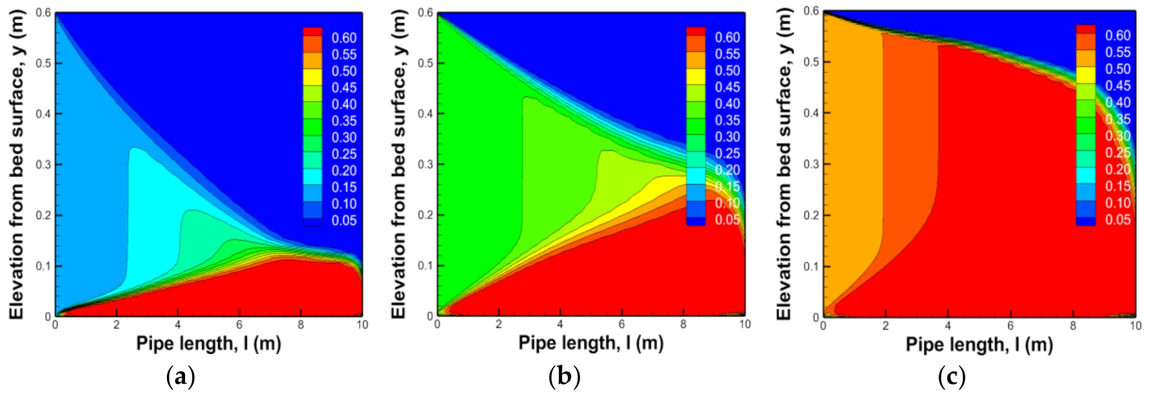
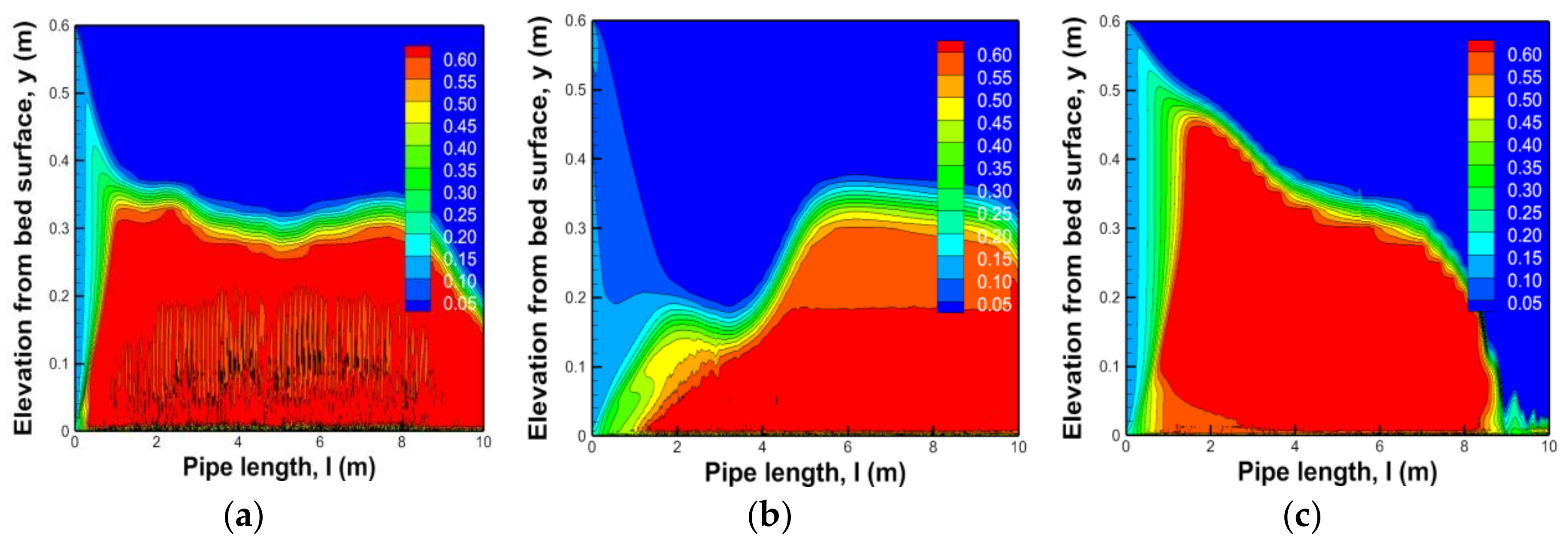
An analysis was carried out to predict the effect and range of soil entering into a conduit on discharge capacity through a transportation and precipitation process. Figure 6, Figure 7, Figure 8 and Figure 9 show the results of numerically simulating depositions in the conduit by assuming transportation and precipitation using a numerical model. In the figure, l is the length of the conduit. Figure 6 and Figure 7 show that the deposit forms in a conduit depending on changes in the volume fractions at the same flow velocity conditions, and list the results of the analysis of 1.0 mm and 20.0 mm as examples.
In Table 5, the observation confirmed that the creation of sections of deposition increased along the direction of the outlet as particle size was relatively small. This means that the range of deposition was created in the same sections due to the effect of turbulent diffusion, which transferred the soil relatively smoothly to the outlet. On the contrary, as the particle size increased, deposition heights were created between the inlet and outlet because the range of turbulent diffusion was small. It was confirmed that the overall discharge capacity decreased according to the increase in volume fractions to block the conduit as the diameter of the soil was large. An increase in the volume fractions can cause a turbulence phenomenon where the flow velocity distribution in the conduit is not uniformly connected to internal deposition.
As particle size increased, the drag force and gravity acting on the particle increased to show larger deposit heights. The largest deposit was located at the end of the conduit as particle size was small. However, as mentioned above, the largest deposit occurring at a particular time moved toward the tail of the conduit over time for all particle sizes.
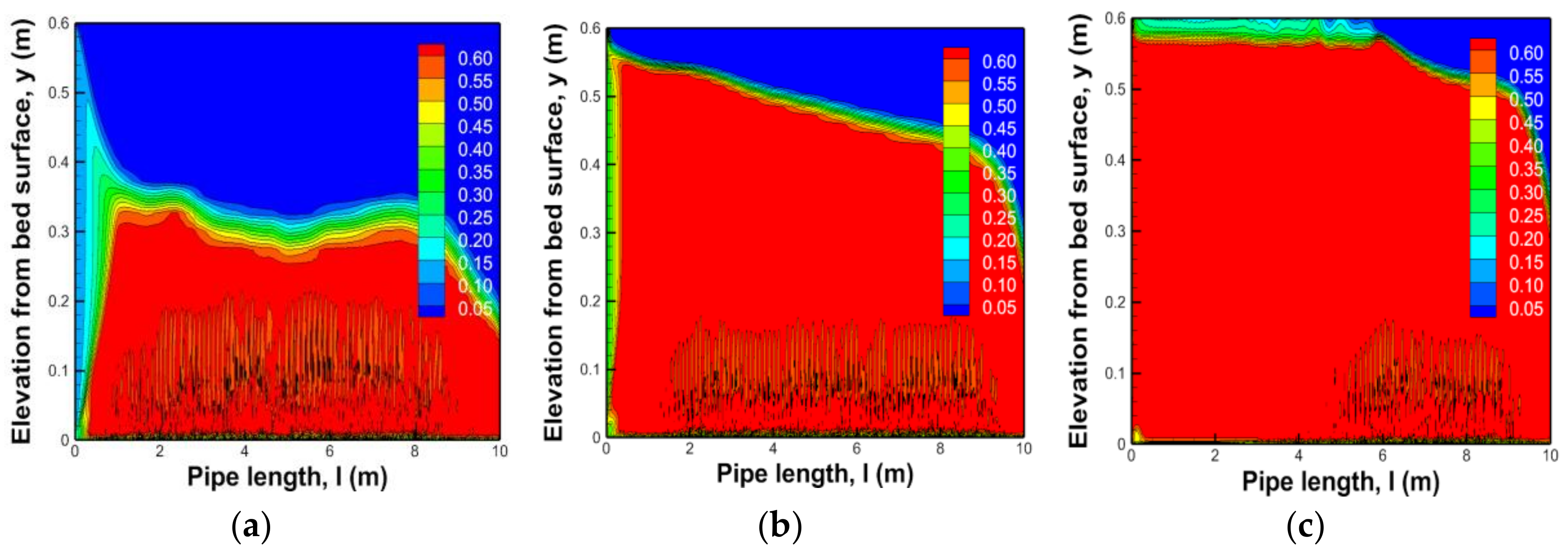
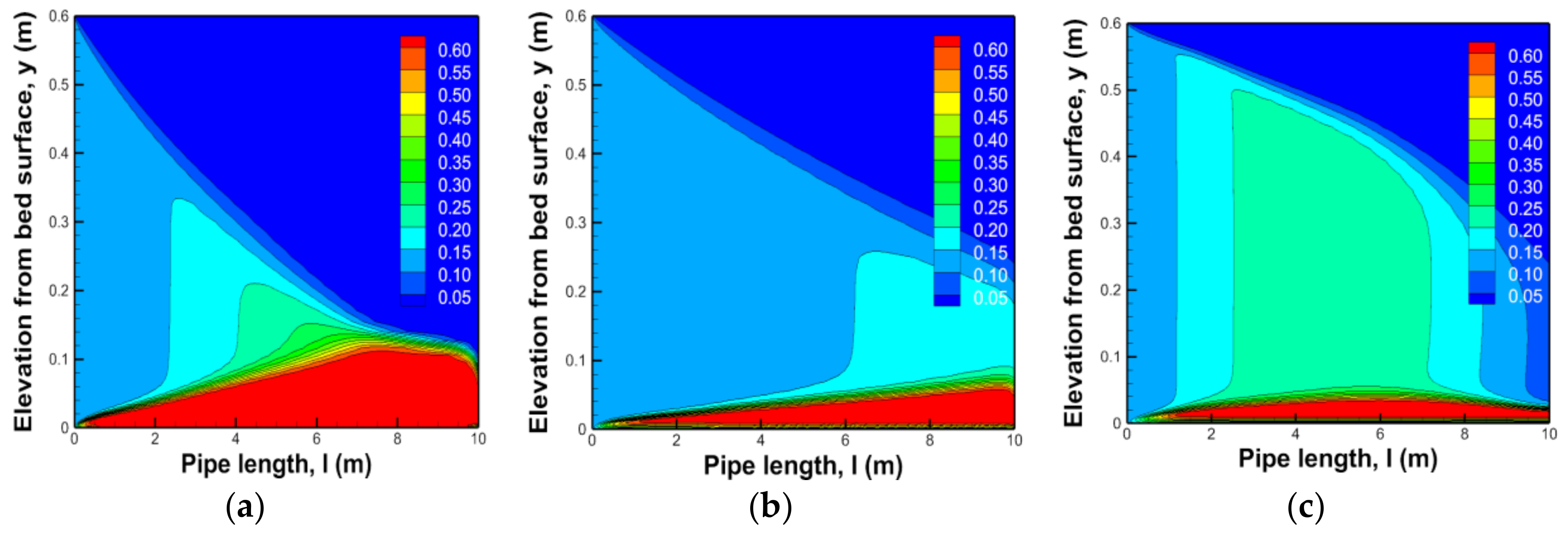
Figure 8 and Figure 9 show the deposition phenomenon in a conduit according to changes in inflow velocity at the same volume fraction and list the results of analysis for soil of diameters 1.0 mm and 20.0 mm as examples. The results show that the deposit height decreased as flow velocity increased. Thus, the force of fluids according to an increase in flow velocity by section was greater than the resistance force of the hardened deposition boundary needed to move the soil, which means an increase in friction owing to an increase in traction.
In Table 6, the results of the numerical analysis confirm that the deposit height increased with particle size and volume fraction of soil and decreased with an increase in flow velocity for the corresponding conditions. An increase in deposit height increased flow velocity at the top of the conduit and, as the size of the soil particles increased, the form of deposition was confirmed. In this event, deposition in a conduit can be said to be a process where soil is rendered cohesive and hardened by viscous force. The section where flows were low at the bottom, according to the deposition, was a bed load, the section where the change in concentration in volume fraction was realized was a suspended load, and that where smooth flows were observed at the top was a wash load.
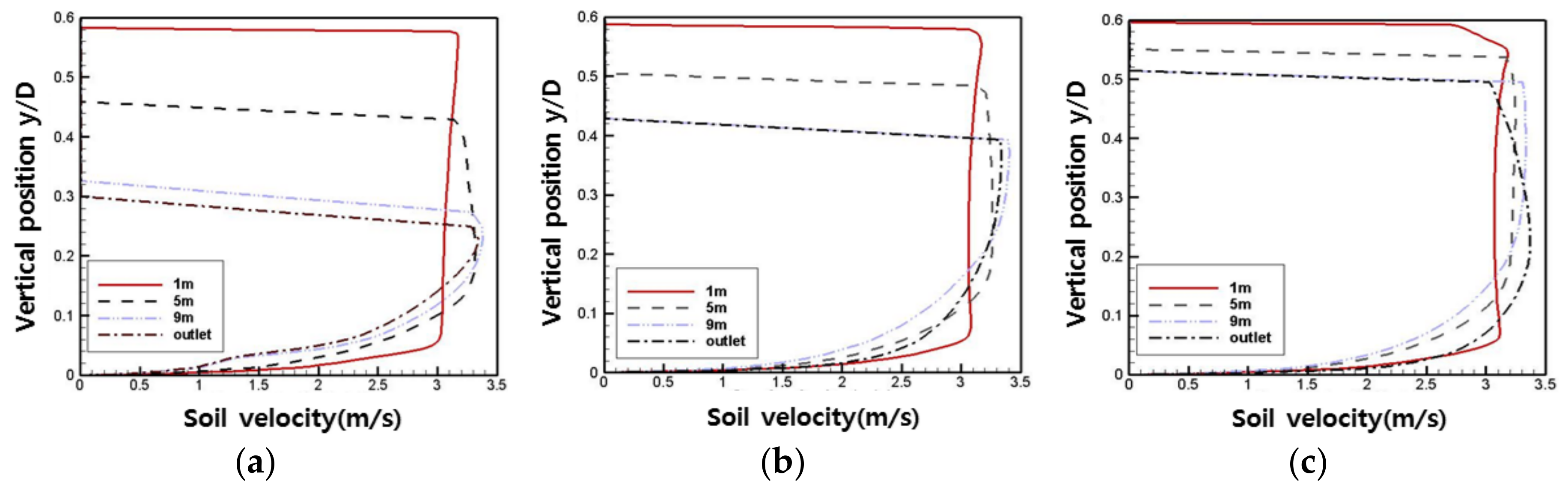
Figure 10 shows the flow velocity distribution of soil along the radial direction at the 1, 5 and 9 m outlet positions along the longitudinal direction of the conduit as the volume fraction of slurry at the inlet was increased to 10%, 30% and 50%, respectively, after fixing the flow velocity of mixtures at 3 m/s and the particle size at 3 mm. y/D refers to a vertical position for a conduit diameter. The biggest differences that depended on changes to the volume fractions of soil at the inlet were in the distribution of soil and its flow velocity in the conduit. The distribution of soil and its flow velocity influenced each other, and the uniformity of the flow velocity distribution indicates the uniformity of particle distribution. In all graphs, for the slurry input uniformly from the inlet, the soil was uniformly distributed over the entire diameter of the conduit (0.6 m), and the flow velocity of soil exhibited the flow characteristics of turbulence.
At conduit lengths of 5 m and 9 m, soil was deposited at the bottom of the conduit as it passed through it so that flow velocity at the top was close to zero, and distribution therein appeared only at a region of deposits smaller than 0.3 m around the outlet (Figure 10a). The flow velocity distribution of soil was considerably distorted from a parabolic form, so that the maximum flow velocity at the 0.3-m position was 3.4 m/s. The radial distribution of soil in the case in Figure 10b was seen to largely increase compared with that in Figure 10a, but the maximum flow velocity of soil occurred at the boundary between soil and water as shown in Figure 9 for the 10% volume fraction. For flow velocity distribution of soil of 50% the volume fraction condition shown in Figure 10c, the distribution of soil was uniform up to the outlet of the conduit along the radial direction, in which case the distribution of soil was confirmed to have a parabolic form. That is, as shown in Figure 10, as the volume fraction at the inlet increased, the flow velocity distribution of mixtures at each position neared a parabolic form, which means that particles were more uniformly distributed in the transverse direction of the conduit.
3.2. Changes in Pattern of Slurry Volume at Outlet
The fluids and soils entering a mixed condition continually changed in forms of distribution as they flowed through the conduit and deposited partially over time. This deposited soil gradually increased in quantity at particular positions of the conduit to cause an increase in local flow velocity at the corresponding section. However, this phenomenon created a repeated form in a conduit to move toward the outlet, and finally discharged. At the end, this pattern was repeated to calculate the amount of deposition; thus, it was necessary to grasp the discharge pattern depending on flow velocity and concentration.
Based on the results of the analysis of 63 cases in this study, the flow distribution of fluids and soils in a conduit were observed to show patterns of discharge of soil deposits from the outlet in three forms.
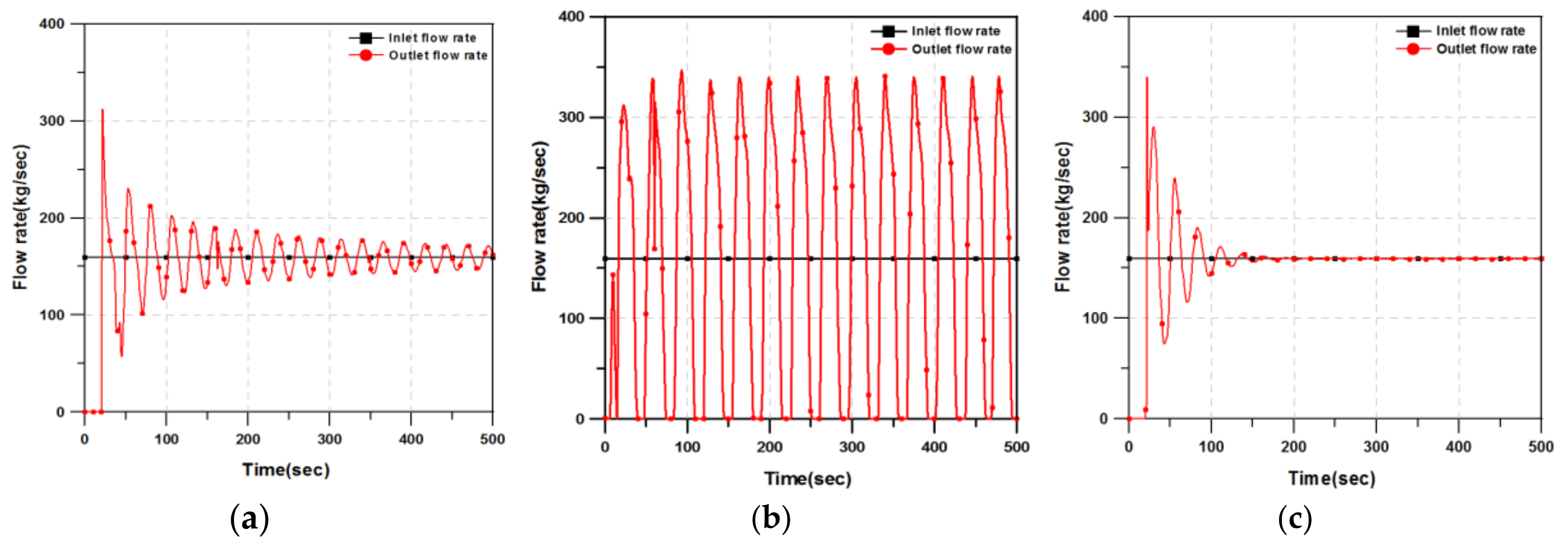
The graph of the inflow/outflow rates of slurry obtained from the obtained results is classified and listed in Figure 11. The first case (Figure 11a) is a pattern where the soil outflow rate formed a cycle with a certain period. This case represents a physical phenomenon whereby the highest deposit of soil occurred at a certain period and discharged from the conduit.
The difference in deposition heights along the longitudinal direction of the conduit was clear. For this physical phenomenon, the inflow velocity should be relatively high and the size of soil particles maintained at a certain level because deposition should occur. Therefore, the phenomenon based on this simulation occurred when the inflow velocity of mixtures was 3 m/s and the size of particles was relatively large. The second case (Figure 11b) shows a pattern where soil discharged at an almost similar, constant rate to the inflow rate without particular changes, excluding the initial stage. The trend of this outlet soil discharge rate appeared primarily when the volume fraction of soil in the mixture was as large as 50% and the inflow velocity of the mixtures was as low as 1.0 m/s. The third case (Figure 11c) is a pattern in which the soil discharge rate gradually decreased at a certain period, similar to the inflow rate after a certain time. This case can be regarded as an interim phenomenon between the first and second trends and appeared when the inflow velocity of mixtures was 2.0 m/s and the volume fraction was 30%.
4. Prediction Model for Height of Particle Deposition in Sewer Conduits
This section is different from the previous sections because the prediction model for height of particle deposition is suggested. This study presents an empirical model formula to predict deposits in conduits of urban drainage systems through a deposition simulation based on inflow rate, volume fraction, and the flow velocities of the fluids and soils entering them. The formula should be able to predict the exact height of the deposit based on theories of transportation and precipitation because the deposition phenomenon during the transportation and precipitation of flowing soils has not been quantified in past studies.
The blocking of a conduit occurs at the position of the highest deposit of soil, not at its average height. This position was calculated at 63 simulation conditions based on volume fractions of soil in a mixture larger than 0.63, a marginal volume fraction of eulerian analysis. The relations between the height of the deposit of soil and the inlet flow velocity of the mixtures, and volume fraction of inlet soil and particle size of soil were derived as correlation equations:
Equation (10) expresses the convective phenomenon in two-phase fluids as a function of particle size and volume fraction using Equation (9) and the Archimedes number based on the minimum fluidization velocity of moving particle . and are the density and viscosity of a moving fluid, is sedimentation velocity, g is gravitational acceleration, and is the density of a moving particle [38].
To derive this correlation equation, nonlinear multivariable regression analysis was carried out, and the inlet flow velocity and particle size in the simulation conditions were non-dimensionalized by Equation (9), with a Reynolds’ number based on particle size. The minimum Reynolds’ number for suspension was obtained using Equation (10) [38], which was used for vertical flows at first. However, given that the diameter of the conduit was 120 times that of the maximum diameter of a particle in this study, it was used for horizontal flows as well. Equation (11) refers to the Archimedes number used in Equation (10).
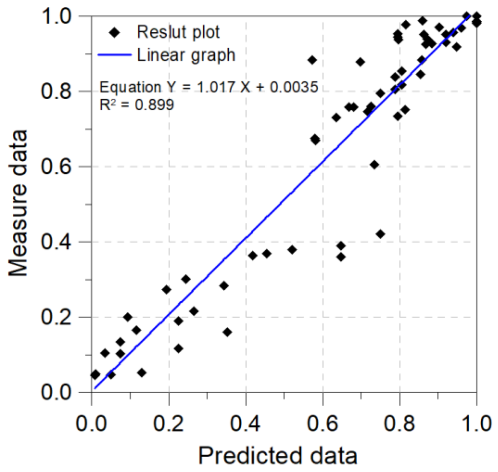
The height of the deposit of soil was non-dimensionalized using conduit diameters in Equation (12). As a result of the linear regression analysis between deposit height and the model, it a correlation coefficient (R2) of 0.877 was obtained. However, in the region where the soil deposition rate y/D was relatively high at 0.4, the deviation in the predictions increased. The rate of deposition increased as the soil volume fraction and particle size increased. Thus, in the analysis, the interaction between the fluids and particles increased, and the deposition height showed small changes compared with various other conditions. Equation (12) can thus be used within the conditions of this analysis, and the flow of soil and slurry had various shapes and sizes of particles. Thus, these results as well as wider operation conditions should be reflected in modeling in future studies.
However, the predicted values in Figure 12 were higher than the measured values in general because the former showed the condition in which blockage in the conduit was maximum. Moreover, the modeled values were closer to the measured values than the predicted values. It can thus be claimed that the modeled values were closer to the measured values than the simply predicted values. Due to this uncertainty, it is necessary to check the suitability of analysis and implement reasonable management through the measured values by establishing a relation between them and the predicted values. By performing a simple regression analysis on the measured data and the predicted data using a prediction formula to verify the usability of the regression equation, a decision coefficient of 0.899 was obtained to indicate high correlation.
The main purpose of this study was to develop a methodology to review flow in a conduit. A performance indicator is the height of the deposit in various conditions of inflow. The methodology should predict the discharge capacity in a conduit and be able to calculate complex features simply. Therefore, a correlation formula considering flow velocity, soil volume fraction, soil diameter, and critical deposit height was developed.
5. Conclusions
An important consideration in planning and designing drainage conduits is to prevent the deposition of soils and sediments entering the conduit. In general, complicated phenomena occur whereby the discharge cross-section of the conduit changes as transportation, precipitation, and deposition occur. To properly design and efficiently maintain drainage conduits, it is necessary to check these phenomena. Analytical research was conducted here on the flow characteristics of slurry in a conduit using the eulerian method, and the following conclusions can be made:
- As the inflow velocity of soil particles in slurry is slow and the particle diameter is large, particles incline to the bottom of the conduit.
- If the soil particles in slurry deposits near the inlet, flow velocity at the deposit increases, according to which the transportation of the deposited soil particles occurs.
- As the flow velocity of incoming slurry is low and the diameter of the soil particles large, the amount of the deposit increases and the stable transportation of slurry is interrupted.
- The relations between the height of the soil deposited and the inlet flow velocity of mixtures, volume fraction of inflowing particle size, which were non-dimensionalized, were derived as a correlation formula.
- Linear regression analysis between the deposit height and the model confirmed a correlation coefficient (R2) of 0.877.
This study conducted analytical research on soil entering a drainage conduit using a numerical analysis model. However, hydrodynamic analysis can be used more effectively than a comparison and review of predicted behavior and can be used to establish an improved plan and design a hydrodynamic structure in several fields. The final aim of this study was to derive a reasonable drainage conduit plan based on an exact theoretical approach and careful analysis.
This result provides the necessary basis for the design of a drainage conduit and the analysis of the blocking or breaking phenomenon of drainage conduits due to disasters such as landslides because of large amount of rainfall in the future. However, to review the flow phenomenon in a drainage conduit by considering the effect of the shapes of various types of soil and debris entering the conduits, it is necessary to review this under various conditions by creating experiments and numerical models. Additionally, an improved sensitivity analysis of sediment parameters could be continued for the explanation of sediment transport as a future study.
Acknowledgments
This research was supported by a grant [MOIS-DP-2015-03] through the Disaster and Safety Management Institute funded by Ministry of the Interior and Safety of Korean government.
Author Contributions
Yang Ho Song carried out the survey of previous studies and wrote the draft of the manuscript. Yang Ho Song and Eui Hoon Lee revised the draft until the final version of the manuscript. Yang Ho Song, Jung Ho Lee and Rin Yun obtained the results. Yang Ho Song, Rin Yun, Eui Hoon Lee and Jung Ho Lee conceived the original idea of the proposed method.
Conflicts of Interest
The authors declare no conflict of interest.
References
- Perrusquia, G. Bedload Transport in Storm Sewers: Stream Traction in Pipe Channels. Ph.D. Thesis, Chalmers University of Technology, Göteborg, Sweden, 11 October 1991. [Google Scholar]
- Nalluri, C.; Ghani, A.A.; El-Zaemey, A. Sediment transport over deposited beds in sewers. Water Sci. Technol. 1994, 29, 125–133. [Google Scholar]
- Kleijwegt, R.A. On Sediment Transport in Circular Sewers with Non-Cohesive Deposits. Ph.D. Thesis, Delft University of Technology, Elft, The Netherlands, 11 May 1992. [Google Scholar]
- Chebbo, G.; Bachoc, A. characterization of suspended soils in urban wet weather discharges. Water Sci. Technol. 1992, 25, 171–179. [Google Scholar]
- Bertrand-Krajewski, J.L.; Barraud, S.; Kouyi, G.L.; Torres, A.; Lepot, M. Online monitoring of particulate pollutant loads in urban sewer systems: Stakes, methods, example of application. La Houille Blanche 2008, 4, 49–57. [Google Scholar] [CrossRef]
- Becouze, L.; Dembele, A.; Coquery, M.; Cren–Olive, C.; Barillon, B.; Bertrand-Krajewski, J.-L. Source characterisation and loads of metals and pesticides in urban wet weather discharges. Urban Water J. 2016, 13, 600–617. [Google Scholar] [CrossRef]
- Nabil, T.; EL-Sawaf, I.; EL-Nahhas, K. Sand-water slurry flow modelling in a horizontal pipeline by computational fluid dynamics technique. Int. Water Technol. J. 2014, 4, 1–17. [Google Scholar]
- Matousek, V. Flow Mechanism of Soil–Water Mixtures in Pipelines. Ph.D. Thesis, Delft University, Delft, The Netherlands, 15 December 1997. [Google Scholar]
- Ota, J.J.; Perrusquia, G. Particle velocity and sediment transport at limit deposition in sewers. In Proceedings of the 12th International Conference on Urban Drainage, Porto Alegre/RS, Brazil, 11–16 September 2011; pp. 1–8. [Google Scholar]
- Kim, C.H.; Han, C.H. Numerical simulation of hydraulic transport of soil–water mixtures in pipelines. Open J. Fluid Dyn. 2013, 3, 266–270. [Google Scholar] [CrossRef]
- Chen, L.; Duan, Y.; Pu, W.; Zhao, C. CFD simulation of coal-water slurry flowing in horizontal pipelines. Korea J. Chem. Eng. 2009, 26, 1144–1154. (In Korean) [Google Scholar] [CrossRef]
- Gopaliya, K.M.; Kaushal, D.R. Modeling of soil-water slurry flow through horizontal pipe using CFD. J. Hydrol. Hydromech. 2016, 64, 261–272. [Google Scholar]
- Onokoko, L.; Galanis, N. CFD prediction of stratification in isothermal ice slurry pipe flow. Int. Refrig. Air Cond. Conf. Purdue 2012, 2525, 1–7. [Google Scholar]
- Shi, X.J.; Zhang, P. Two-phase flow and heat transfer characteristics of tetra-n-butyl ammonium bromide clathrate hydrate slurry in horizontal 90° elbow pipe and U-pipe. Int. J. Heat Mass Transf. 2016, 97, 364–378. [Google Scholar] [CrossRef]
- Tian, Q.; He, G.; Wang, H.; Cai, D. Simulation on transportation safety of ice slurry in ice cooling system of buildings. Energy Build. 2014, 72, 262–270. [Google Scholar] [CrossRef]
- Kaushal, D.R.; Tomita, Y.; Dighade, R.R. Concentration at the pipe bottom at deposition velocity for transportation of commercial slurries through pipeline. Power Technol. 2002, 125, 89–101. [Google Scholar] [CrossRef]
- Lorenzen, A.; Ristenpart, E.; Pfuhl, W. Flush cleaning of sewers. Water Sci. Technol. 1996, 33, 221–228. [Google Scholar]
- Bertrand-Krajewski, J.L.; Campisano, A.; Creaco, E.; Modica, C. Experimental analysis of the Hydrass flushing gate and field validation of flush propagation modelling. Water Sci. Technol. 2005, 51, 129–137. [Google Scholar] [PubMed]
- Dettmar, J.; Staufer, P. Modelling of flushing waves for optimising cleaning operations. Water Sci. Technol. 2005, 52, 233–240. [Google Scholar] [PubMed]
- Campisano, A.; Creaco, E.; Modica, C. Numerical modelling of sediment bed aggradation in open rectangular drainage channels. Urban Water J. 2013, 10, 365–376. [Google Scholar] [CrossRef]
- Raquel, I.S. In-Sewer Organic Sediment Transport. Ph.D. Thesis, Universitat Politècnica de Catalunya Barcelona Tech, Barcelona, Spain, October 2014. [Google Scholar]
- Crowe, C.T.; Schwarzkopf, J.D.; Sommerfeld, M.; Tsuji, Y. Multiphase Flows with Droplets and Particles, 2nd ed.; CRC Press: Boca Raton, FL, USA, 2012; pp. 8–9. [Google Scholar]
- ANSYS. ANSYS Fluent 12.1 Theory Guide; ANSYS, Inc.: Canonsburg, PA, USA, 2010. [Google Scholar]
- Versteeg, H.K.; Malalasekera, W. An Introduction to Computational Fluid Dynamics, 2nd ed.; Pearson Education Limited: Hongkong, China, 2007. [Google Scholar]
- Boris, V.B.; Alex, C.H.; Pawel, K.; Lee, D.R. Eulerian–Eulerian CFD model for the sedimentation of spherical particles in suspension with high particle concentrations. Eng. Appl. Comput. Fluid Mech. 2010, 4, 116–126. [Google Scholar]
- Lixing, Z. Two-phase turbulence models in Eulerian–Eulerian simulation of gas particle flows and coal combustion. Procedia Eng. 2015, 102, 1677–1696. [Google Scholar]
- Zhen, C.; Tian-Jian, H.; Joseph, C. SedFoam. A multi-dimensional Eulerian two-phase model for sediment transport and its application to momentary bed failure. Coast. Eng. 2017, 119, 32–50. [Google Scholar]
- Everitt, B.S.; Hand, D. Finite Mixture Distributions; Wiley & Sons, Inc.: London, UK, 1985. [Google Scholar]
- Jones, W.P.; Launder, B.E. The Prediction of Laminarization with a Two-Equation Model of Turbulence. Int. J. Heat Mass Transf. 1972, 15, 301–314. [Google Scholar] [CrossRef]
- Syamlal, M.; O’Brien, T.J. Fluid dynamic simulation of O3 decomposition in a bubbling fluidized bed. AIChE J. 2003, 49, 2793–2801. [Google Scholar] [CrossRef]
- Syamlal, M.; O’Brien, T.J. The Derivation of a Drag Coefficient from Velocity-Voidage Correlation; National Energy Technology Laboratory: Morgantown, WV, USA, 1994; Unpublished Report. [Google Scholar]
- Syamlal, M.; O’Brien, T.J. Computer simulation of bubbles in a fluidized bed. AIChE J. 1989, 85, 22–31. [Google Scholar]
- Taghipour, F.; Ellis, N.; Wong, C. Experimental and computational study of gas–soil fluidized bed hydrodynamics. Chem. Eng. Sci. 2005, 60, 6857–6867. [Google Scholar] [CrossRef]
- Hernández-Jiménez, F.; Sánchez-Delgado, S.; Gómez-García, A.; Acosta-Iborra, A. Comparison between two-fluid model simulations and particle image analysis and velocimetry (PIV) results for a two-dimensional gas–soil fluidized bed. Chem. Eng. Sci. 2011, 66, 3753–3772. [Google Scholar]
- Kalambe, A.R. Two-Phase Flow CFD Analysis of Refrigerants in a Condenser Pipe for Prediction of Pressure Drop and Pumping Power. Master’s Thesis, The University of Texas, Arlington, TX, USA, 2015. [Google Scholar]
- Wilcox, D.C. Turbulence Modeling for CFD; DCW Industries, Inc.: La Cãnada, CA, USA, 2006. [Google Scholar]
- Park, C.W.; Hong, C.H. User Guide of ANSYS Workbench; Intervision: Seoul, Korea, 2008.
- Wen, C.Y.; Yu, Y.H. A generalized method for predicting the minimum fluidization velocity. AIChE. J. 1966, 12, 610–612. [Google Scholar] [CrossRef]
Figure 1.
Horizontal pneumatic transport. (a) Homogeneous flow; (b) Dune flow; (c) Slug flow.

Figure 2.
Flowchart of analysis procedure.

Figure 3.
Comparison of the velocity of the simulated mixture (m/s) with that in experimental results [7].
Figure 3.
Comparison of the velocity of the simulated mixture (m/s) with that in experimental results [7].

Figure 4.
Comparison of the simulated soil volume fraction (%) with that in experimental results [7].
Figure 4.
Comparison of the simulated soil volume fraction (%) with that in experimental results [7].

Figure 5.
Conduit mesh.

Figure 6.
Sedimentation results for soil of diameter 1.0 mm according to changes in volume fraction; (a) Volume fraction 10%; (b) Volume fraction 30%; (c) Volume fraction 50%.
Figure 6.
Sedimentation results for soil of diameter 1.0 mm according to changes in volume fraction; (a) Volume fraction 10%; (b) Volume fraction 30%; (c) Volume fraction 50%.

Figure 7.
Sedimentation results for soil of diameter 20.0 mm according to changes in volume fraction. (a) Volume fraction 10%; (b) Volume fraction 30%; (c) Volume fraction 50%.
Figure 7.
Sedimentation results for soil of diameter 20.0 mm according to changes in volume fraction. (a) Volume fraction 10%; (b) Volume fraction 30%; (c) Volume fraction 50%.

Figure 8.
Sedimentation results for soil of diameter 1.0 mm according to changes in inlet velocity. (a) 1.0 m/s inlet velocity; (b) 2.0 m/s inlet velocity; (c) 3.0 m/s inlet velocity.
Figure 8.
Sedimentation results for soil of diameter 1.0 mm according to changes in inlet velocity. (a) 1.0 m/s inlet velocity; (b) 2.0 m/s inlet velocity; (c) 3.0 m/s inlet velocity.

Figure 9.
Sedimentation results for soil of diameter 20.0 mm according to changes in inlet velocity. (a) 1.0 m/s inlet velocity; (b) 2.0 m/s inlet velocity; (c) 3.0 m/s inlet velocity.
Figure 9.
Sedimentation results for soil of diameter 20.0 mm according to changes in inlet velocity. (a) 1.0 m/s inlet velocity; (b) 2.0 m/s inlet velocity; (c) 3.0 m/s inlet velocity.

Figure 10.
Soil velocity and soil diameter according to change in volume fraction. (a) Soil velocity distribution at a volume fraction of 10%; (b) Soil velocity distribution at a volume fraction of 30%; (c) Soil velocity distribution at a volume fraction of 50%.
Figure 10.
Soil velocity and soil diameter according to change in volume fraction. (a) Soil velocity distribution at a volume fraction of 10%; (b) Soil velocity distribution at a volume fraction of 30%; (c) Soil velocity distribution at a volume fraction of 50%.

Figure 11.
Flow patterns and characteristics diagram in sewer. (a) Moderately damped oscillation; (b) Oscillation pattern; (c) Highly damped oscillation pattern.
Figure 11.
Flow patterns and characteristics diagram in sewer. (a) Moderately damped oscillation; (b) Oscillation pattern; (c) Highly damped oscillation pattern.

Figure 12.
Correlations between simulated results and predicted results by Equation (12).


Table 1.
Standard k–ε model parameters.
| 0.09 | 1.44 | 1.92 | 1.0 | 1.3 |
Table 2.
Conditions of analysis in FLUENT.
| Condition | Setting |
|---|---|
| Type | Fluid |
| Material | Water |
| Turbulence Model | k–ε standard |
| Inlet | Velocity = 1.0–3.0 m/s |
| Outlet | Relative pressure = 0 (Pa) |
| Wall Influence of Flow | No slip |
| Surface Influence of Flow | Free slip |
Table 3.
Simulation conditions for comparison with experimental results.
| Title | Soil–Water Transport |
|---|---|
| Geometry | 10.55 m × 0.015 m |
| Model | Eulerian–eulerian model, Turbulent flow |
| Mixture boundary Conditions | Inlet velocity: 3 m/s, Inlet volume fraction: 30% |
| Soil | Density: 2650 kg/m3, Particle diameter: 0.2 mm |
| Water | Density: 1000 kg/m3, Dynamic viscosity: 0.001004 Pa·s |
Table 4.
Parameters of standard k–ε model.
| Titles | Conditions | |
|---|---|---|
| Geometry | 0.6 m (D) × 10 m (L) | |
| Model | Eulerian–eulerian model, Turbulent flow | |
| Mixture boundary Conditions | Inlet Velocity (m/s): | 1.0, 2.0, 3.0 |
| Inlet Volume Fraction (%): | 10, 30, 50 | |
| Soil | Density (kg/m3): | 2650 |
| Particle Diameter (mm): | 0.5, 1.0, 3.0, 5.0, 7.0, 15.0, 20.0 | |
| Water | Density (kg/m3): | 1000 |
| Dynamic Viscosity (Pa·s): | 0.001004 | |
Table 5.
Sedimentation results for soil of diameter 1.0 mm and 20.0 mm according to changes in volume fraction (where the soil deposition rate h/D).
Table 5.
Sedimentation results for soil of diameter 1.0 mm and 20.0 mm according to changes in volume fraction (where the soil deposition rate h/D).
| Volume Fraction | 10 | 30 | 50 | |
|---|---|---|---|---|
| D (mm) | ||||
| 1.0 | 0.160 | 0.365 | 0.884 | |
| 20.0 | 0.629 | 0.938 | 0.967 | |
Table 6.
Sedimentation results for soil of diameter 1.0 mm according to changes in inlet velocity (where the soil deposition rate h/D).
Table 6.
Sedimentation results for soil of diameter 1.0 mm according to changes in inlet velocity (where the soil deposition rate h/D).
| Velocity (m/s) | 1.0 | 2.0 | 3.0 | |
|---|---|---|---|---|
| D (mm) | ||||
| 1.0 | 0.160 | 0.053 | 0.047 | |
| 20.0 | 0.629 | 0.552 | 0.518 | |
© 2018 by the authors. Licensee MDPI, Basel, Switzerland. This article is an open access article distributed under the terms and conditions of the Creative Commons Attribution (CC BY) license (http://creativecommons.org/licenses/by/4.0/).
Share and Cite
MDPI and ACS Style
Song, Y.H.; Yun, R.; Lee, E.H.; Lee, J.H. Predicting Sedimentation in Urban Sewer Conduits. Water 2018, 10, 462. https://doi.org/10.3390/w10040462
AMA Style
Song YH, Yun R, Lee EH, Lee JH. Predicting Sedimentation in Urban Sewer Conduits. Water. 2018; 10(4):462. https://doi.org/10.3390/w10040462
Chicago/Turabian StyleSong, Yang Ho, Rin Yun, Eui Hoon Lee, and Jung Ho Lee. 2018. "Predicting Sedimentation in Urban Sewer Conduits" Water 10, no. 4: 462. https://doi.org/10.3390/w10040462
Note that from the first issue of 2016, this journal uses article numbers instead of page numbers. See further details here.