Multi-Objective Validation of SWAT for Sparsely-Gauged West African River Basins—A Remote Sensing Approach


1
Department of Geography, University of Bonn, Meckenheimer Allee 166, 53115 Bonn, Germany
2
Institute of Geodesy and Geoinformation, University of Bonn, Nussallee 17, 53115 Bonn, Germany
3
Geodäsie und Ausgleichsrechnung, HafenCity University Hamburg, Überseeallee 16, 20457 Hamburg, Germany
*
Author to whom correspondence should be addressed.
Water 2018, 10(4), 451; https://doi.org/10.3390/w10040451
Submission received: 22 February 2018
/
Revised: 15 March 2018
/
Accepted: 5 April 2018
/
Published: 9 April 2018
(This article belongs to the Special Issue Hydrological Modelling and Remote Sensing: Selected Papers from the 2017 and 2018 SWAT International Conferences)
Abstract
:Predicting freshwater resources is a major concern in West Africa, where large parts of the population depend on rain-fed subsistence agriculture. However, a steady decline in the availability of in-situ measurements of climatic and hydrologic variables makes it difficult to simulate water resource availability with hydrological models. In this study, a modeling framework was set up for sparsely-gauged catchments in West Africa using the Soil and Water Assessment Tool (SWAT), whilst largely relying on remote sensing and reanalysis inputs. The model was calibrated using two different strategies and validated using discharge measurements. New in this study is the use of a multi-objective validation conducted to further investigate the performance of the model, where simulated actual evapotranspiration, soil moisture, and total water storage were evaluated using remote sensing data. Results show that the model performs well (R2 calibration: 0.52 and 0.51; R2 validation: 0.63 and 0.61) and the multi-objective validation reveals good agreement between predictions and observations. The study reveals the potential of using remote sensing data in sparsely-gauged catchments, resulting in good performance and providing data for evaluating water balance components that are not usually validated. The modeling framework presented in this study is the basis for future studies, which will address model response to extreme drought and flood events and further examine the coincidence with Gravity Recovery and Climate Experiment (GRACE) total water storage retrievals.
1. Introduction
The availability of freshwater is a major concern in West Africa, directly influencing food security, human health, and economic development [1]. In the region, approximately 60% of the active labor force is employed in agriculture. However, this only contributes 35% to the gross domestic product [2,3]. Many West African farmers are poor and only able to produce close to subsistence levels, rendering them especially vulnerable to water stress [3]. Therefore, knowledge of the available water resources is essential and modeling the water balance to estimate available resources can be an important tool in this respect. Several meso-scale models have been applied to the area, among others by Andersen et al., who used the physically-based MIKE SHE model to model the Senegal river basin in 2001 [4]. In 2005, Bormann studied the results of two process-based (SIMULAT-H and TOPLATS) and one conceptual hydrological model (UHP) applied to the upper Ouémé basin [5]. Another approach was employed by Wagner et al., who downscaled meteorological fields and remote sensing data over the White Volta basin for water balance estimation [6]. Due to the lack of in-situ data in the region, remote sensing data is starting to be used more often for water resource estimation, e.g., by Fujihara et al., who used reanalysis and global precipitation data in 2014 to model the White Volta basin [7]. The estimation of available water resources has furthermore been a topic of research for the whole of West Africa in several studies, e.g., by Döll et al., who used the WaterGAP Global Hydrology Model to estimate water resources worldwide [8] or Li et al., who used the IBIS land surface model in combination with the hydrological HYDRA model for the Niger and Lake Chad basins [9]. However, calibrating global hydrological models against long-term annual discharge may lead to poor temporal performance [1].
Considering these constraints, Schuol et al. employed the semi-distributed, physically-based hydrological SWAT (Soil & Water Assessment Tool) model to estimate freshwater resources of West Africa in 1998 [1,10]. The model was later expanded to cover the whole of Africa [11] and a calibration/validation approach of this model using GRACE gravity recovery data was performed by Xie et al., who found SWAT and GRACE agreeing less in arid and humid regions, albeit using historic discharge data for the modern period simulated [12]. In their approach, Schuol et al. covered a four mio. km2 research area in West Africa, which was partitioned into 292 sub-basins. Inaccurate or missing input data have been shown to increase uncertainties of distributed hydrological models [13,14]. Especially in developing countries, observation networks are sparse, and data regularly includes gaps and gross errors [15,16,17]. A continuous decline in data availability has been observed in recent years due to political unrest, financial issues, and maintenance problems [18,19]. Schuol et al. circumvented this data availability problem by training a weather generator to produce daily data using 0.5° Climate Research Unit monthly data [13]. While some authors state that hydrological models may perform poorly due to the limited data availability in the region [20], Schuol et al. demonstrated the SWAT model to deliver robust results [1,10,11].
In recent years, many studies have explored the performance of remotely sensed climate data in Africa, with the focus being on the evaluation of precipitation estimates. Investigations have been conducted, among others, for West Africa [7,21,22,23,24], East Africa [17,21,25,26,27], Southern Africa [28], and the entire continent [29]. Most studies agree that certain precipitation products perform well and may be used in substituting for in-situ gauge data. However, in regions with complex topography and strong altitude variations over short distances, as e.g., in Ethiopia, the performance of satellite precipitation estimates declines sharply [25,27]. We hypothesize that the increasing number of high resolution remote sensing data products will enable substituting data from gauge networks and render weather generators, as used in the study by Schuol et al. [13], obsolete. In this study, we set up a modeling framework by calibrating and validating a SWAT model covering the major West African river basins for the period of 1998–2013, using freely available remote sensing and reanalysis products including new climatological, land use, and soil datasets. The starting time is restricted due to the availability of high resolution satellite data and the end of the modeling period is determined by the lack of discharge data for model validation. While we have chosen to use only freely available data to guarantee the best-possible applicability of the framework, we realize that finding the appropriate discharge data to validate the model is a challenge. To overcome this problem, a multi-objective validation was conducted, where in addition to streamflow, the variables actual evapotranspiration, soil moisture and total water storage were used to test the model results against available satellite datasets. Therefore, the objectives of this study are (i) to set up a hydrological modeling framework for West Africa using freely available data, (ii) to assess which simulation quality can be obtained using these datasets, (iii) to perform a multi-objective validation, and (iv) to evaluate the potential and limitations of this approach for assessing water availability at the sub-continental scale.
2. Materials and Methods
2.1. Research Area
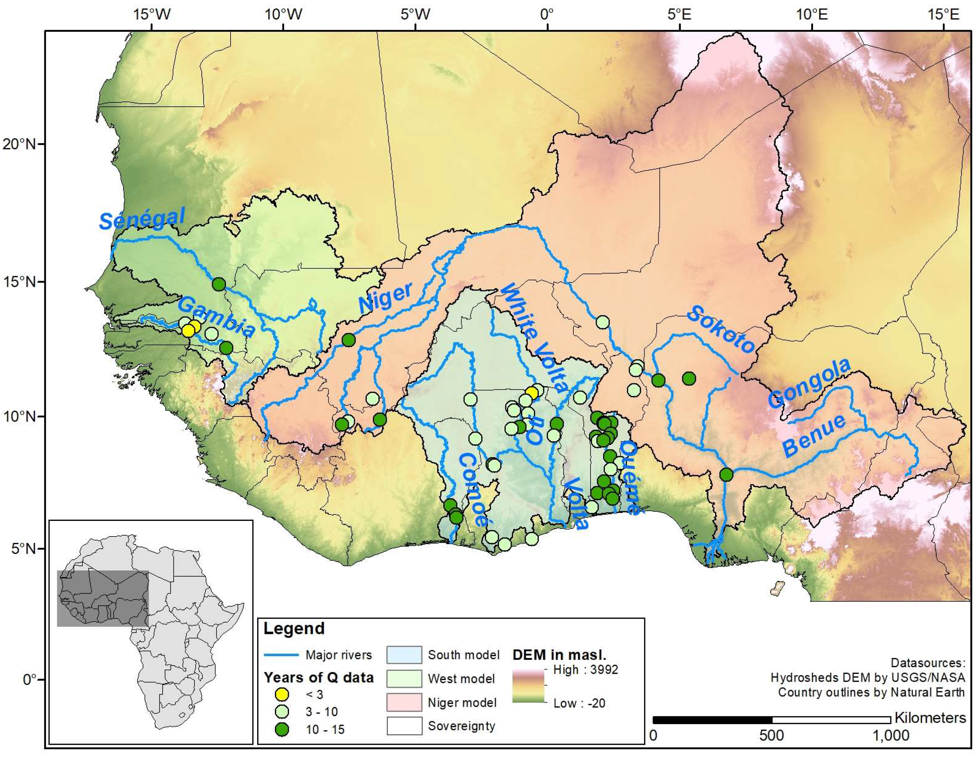
The research area is located between 3° and 24° latitude and −18° and 16° longitude and includes, among others, the basins of the Niger, Volta, Senegal and Ouémé rivers stretching over 18 countries, as shown in Figure 1. The relief in West Africa is low and flat [30] and rainfall is strongly seasonal, with a unimodal rainy season in the northern part and bimodal rainy seasons in the south [31]. Rainfall amounts show a distinct south-north gradient. Annual average precipitation in the humid Guinea-Congolian region in the south ranges from 2200 to 5000 mm, while in the arid Sahara region, annual rainfall ranges from 0 to 150 mm [30,32,33].
River basins were selected based on the availability of discharge data for calibration purposes. The total area of the basins selected for the model is 3.4 mio. km2. Due to computational constraints, three different models were built: South (Volta, Ouémé, Comoé, Mono, Pra, Ankobra and Ayensu river basins, 633,000 km2, 41 stream gauges), West (Senegal and Gambia river basins, 558,600 km2, 9 stream gauges) and Niger (Niger river basin, 2,250,000 km2, 12 stream gauges).
2.2. The SWAT Hydrological Model
The Soil and Water Assessment Tool (SWAT) represents a continuous-time, semi-distributed, process-based river basin model. SWAT runs at a daily time step but may be calibrated using monthly or yearly observed data [34,35]. The model is comprised of eight major components: hydrology, weather, sedimentation, soil temperature and properties, crop growth, nutrients, pesticides and agricultural management. The hydrological component of SWAT is based on the water balance equation [14]. SWAT has been proven to be competitive at a number of scales from local to continental, having been employed for the modeling of water resources in Africa and Europe [11,36], among others. In this study, SWAT 2012 was used. The major model inputs and data preparation will be described in detail below.
2.3. Input Datasets
- Digital Elevation Model (DEM): The hydrologically conditioned HydroSHEDS (Hydrological data and maps based on SHuttle Elevation Derivatives at multiple Scales) digital elevation model (DEM) developed by the World Wildlife Fund (WWF) and the United States Geological Survey (USGS) based on the NASA SRTM (Shuttle Radar Topographic Mission) was used for streamflow delineation. HydroSHEDS is available in 3 and 15 arc-second resolutions (approximately 90 and 500 m) [37,38]. In this study, sub-basins were generated using the 500 m version.
- Land use and land cover: The Comité permanent Inter-Etats de Lutte contre la Sécheresse dans le Sahel (CILSS) Landscapes of West Africa land use and land cover raster dataset of the year 2013 was used as a basis for developing the land use layer required by SWAT. Maps are also available for the years 1975 and 2000 at a resolution of 2 km. The maps were created using local information and remote sensing data in cooperation with US Aid and USGS [30]. Since no data is included for the country of Cameroon, nor north of the 18th parallel in Mauritania and Mali and north of the 15.5th parallel in Niger, missing data was replaced using the European Space Agency (ESA) Globcover 2.3 dataset depicting the land use of the year 2009 in a 300 m resolution [39]. Land use classes were converted to default SWAT classes. It is unclear whether SWAT allows to realistically simulate plant growth under tropical conditions due to its implemented heat unit growth model [40,41,42]. In our study, the management database was adapted by setting fixed plant and harvest dates corresponding to onset and end of rainy season. When compared to MODerate-resolution Imaging Spectroradiometer (MODIS) MOD 15A2 leaf area index (LAI) estimates produced by NASA [43], SWAT LAI reaches a Pearson’s r of 0.62, whereas without management modifications this value drops to −0.47.
- Soil: The Harmonized World Soil Database (HWSD) version 1.2 produced by the Food and Agriculture Organization of the United Nations, the International Institute for Applied Systems Analysis, ISRIC World Soil Information, the Institute of Soil Science—Chinese Academy of Sciences and the European Commission’s Joint Research Centre (JRC) in 2012 was used to generate the soil data needed in SWAT. The HWSD supplies a raster map and database containing several soil physical and chemical parameters for a top- and subsoil layer [44]. Missing parameters were estimated from soil texture using pedotransfer functions [45]. The HWSD and its predecessors have been used for SWAT simulations in Africa, the Middle East, and Europe, among others [1,11,12,36,46,47,48].
- Climate: In a previous study, ten precipitation datasets were analyzed for six sub-basins in the study area [23]. It was concluded that the Climate Prediction Center Morphing Technique (CMORPH) version 1 CRT produced by the National Oceanic and Atmospheric Administration Climate Prediction Centre (NOAA-CPC) performed best. CMORPHv1 CRT is a global precipitation analysis algorithm, including satellite infrared and microwave precipitation estimates as well as rain gauge information for bias correction. Precipitation estimates are available from 1998 onwards at a resolution of 0.25° [49,50]. Minimum and maximum 2 m daily temperature data were compiled from the NASA MERRA 2 reanalysis dataset. Inputs from both satellite and ground data are included at a resolution of 0.625° × 0.5° [51]. While SWAT-ready climate input files based on the National Centers for Environmental Prediction (NCEP) climate forecast system reanalysis data (CFSR) [52] are readily available, as discovered in Poméon et al. [23], CFSR precipitation information compares worse to other products in the region. No other climate data were necessary as the authors selected Hargreaves as the potential evapotranspiration method.
- Discharge and reservoirs: Discharge data used in this study was obtained from the German Global Runoff Data Center (GRDC) in Koblenz, the French AMMA-CATCH regional observing system, as well as through personal communication with local agencies. Discharge stations and their temporal coverage (without gaps) are depicted in Figure 1 and summarized in Table 1. The 12 largest reservoirs in the study area where downstream discharge observations are available were included in the model. Reservoir information was provided by the Global Water System Project (GWSP) Global Reservoir and Dam (GRanD) database version 1.1 created by Lehner et al. [53]. Missing storage volumes information was approximated as proposed by Schuol et al. [1]. Lake Volta was not modeled due to insufficient data being available.
2.4. Multi-Objective Validation Datasets
We decided to validate model simulations using actual evapotranspiration, soil moisture, and total water storage, in order to evaluate the model performance of processes not reflected in streamflow. This section gives an overview of the remote sensing data used in the multi-objective validation.
- Actual evapotranspiration (ETa): Data was extracted from the MODIS MOD 16 dataset supplied by NASA, available at a 1 km2 spatial- and 8-day or monthly temporal resolution. ETa is calculated based on the Penman-Monteith equation using ground-based and remote sensing datasets. The algorithm includes vapor pressure deficit, leaf area index, enhanced vegetation index and soil evaporation [54,55].
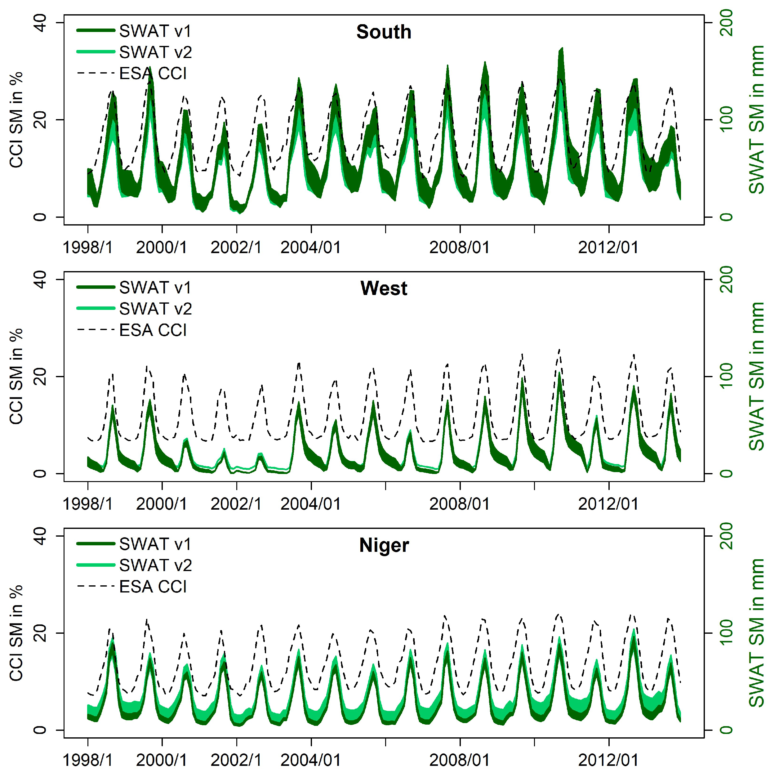
- Soil moisture: ESA Climate Change Initiative (CCI) 3.2 soil moisture (SM) retrievals were used to validate the soil moisture dynamics simulated by SWAT. The product is generated by blending passive and active microwave soil moisture retrievals generated by C-band scatterometers and multi-frequency radiometers on multiple spacecraft. Daily data is available at a resolution of 0.25 degrees but covering only the upper few cm of the soil [56,57,58].
- Total water storage (TWS): Gravity Recovery And Climate Experiment (GRACE) TWS retrievals were used for further model validation. The twin satellite GRACE mission has been measuring temporal and spatial variations in the Earth’s gravity field since 2002. GRACE consists of two identical satellites on the same near-circular orbit. The dual one-way K-band microwave ranging system observes the distance between the two satellites. Changes in the distance in conjunction with complementary tracking data are used to derive monthly gravity fields, which, subsequently, are converted to mass changes in terms of equivalent water height according to Wahr et al. [59]. In this study, we used the ITSG-Grace2016 time series provided by the Institute of Geodesy (IfG) at Technical University (TU) Graz as sets of spherical harmonic coefficients up to degree and order 90. As GRACE does not measure geocenter variations, degree 1 coefficients were replaced by the time series provided by Rietbroek et al. [60,61]. The c20 coefficient, which is corrupted by aliasing effects, was replaced by results from satellite laser ranging [62]. GRACE observes the integral sum of all mass variations in hydrosphere, atmosphere, biosphere, oceans and mass variations inside of the earth. Gravity field solutions from ITSG-Grace2016 are already corrected for tides (ocean, earth and pole tides) and non-tidal atmospheric and oceanic effects. Trends from glacial isostatic adjustment are about zero in the study region. Therefore, the spherical harmonic coefficients from ITSG-Grace2016 primarily reflect variations in the terrestrial water storage. As GRACE-derived gravity solutions are contaminated with correlated noise leading to the characteristic striping patterns in the north-nouth direction, the monthly fields were smoothed using the anisotropic DDK3 filter [63]. Filtering implies attenuation of the signal and further distortion, known as leakage effect. Therefore, TWS time series derived for the three target areas via spatial averaging were rescaled using the scaling factor approach [64]. Here, scaling factors were derived from five global hydrological models for each target area separately [65]. All computations are accompanied by a thorough error propagation, which starts from the full error covariance matrices of the spherical harmonic coefficients and results into errors for the rescaled TWS time series. Since Lake Volta was not modeled in SWAT, the lake signal was computed using lake height variations and an area varying between 4450 km2 and 9970 km2 [66,67] and subsequently subtracted from the GRACE estimates.
2.5. Model Setup and Calibration/Validation
The model parametrization was conducted using the ArcSWAT 2012 interface [68]. The research areas were divided into sub-basins based on the DEM and derived stream network. We used a streamflow delineation threshold of at least 500 km2 for the southern and western models (1500 km2 for the Niger model) and manually added outlets where data from gauging stations was available, generating 2153 sub-basins (South: 712; West: 630; Niger: 811). Next, the sub-basins were overlaid with land use and soil maps to derive Hydrological Response Units (HRUs), units with the same land use, soil and slope characteristics [40]. In view of computational efficiency, we opted to derive one HRU per sub-basin by considering dominant land use, soil and slope [11] (divided into 0–1; >1–5 and >5% slope).
The dominant land use distribution for each model is displayed in Figure 2. In the South model, range-brush is the dominant land use type (53.6%), followed by agriculture (31.4%) and forest (7.8%). Both forest and agricultural areas are mostly located in the more humid south, while rangeland dominates in the arid north. In the western model, rangeland (brush and grasses) dominates with 40.4 and 47.8%, respectively. 8.6% of the area is barren and 2.9% under agricultural use. Land use in the Niger model is to almost equal parts range grasses, barren, agriculture and range brush (26.4, 24.6, 23.3 and 22.2%). The high prevalence of barren areas can be explained by the hydrologically inactive part of the basin, located in the north-east [69]. Only 2.6% of the area is predominantly forested.
After generating the HRUs, reservoirs were included as described in Section 2.3. Due to uncertainties in the climate data, the potential evapotranspiration was calculated using the 1985 Hargreaves equation, which requires only temperature and extraterrestrial radiation inputs [40,70]. In SWAT, extraterrestrial radiation is calculated as a function of location and time of year [40]. The Hargreaves method has been suggested if the input data quality is in doubt [71]. Since the evapotranspiration processes in the study region are water-limited, more emphasis should be placed on the actual evapotranspiration, as it directly influences runoff generation [72]. SWAT calculates the Hargreaves (1985) equation as follows (Equation (1)):
where is the latent heat of vaporization in MJ/kg, is the potential evapotranspiration in mm, is the extraterrestrial radiation in MJ/m2, is the maximum air temperature in °C, is the minimum air temperature in °C, and is the average air temperature in °C [40].
The simulation covered the period of 1998 to 2013 with a warm-up period from 1996 to 1997. Since CMORPH precipitation data was only available from 1998 onwards, data from 1998 to 1999 was used as fictitious data for the warm-up period in order to maximize the simulation period.
The calibration of a semi-distributed watershed model such as SWAT is challenging due to input uncertainties, model uncertainties and parameter non-uniqueness [10,73]. For the calibration of our models, the Sequential Uncertainty Fitting version 2 (SUFI-2) procedure of SWAT-CUP (Calibration and Uncertainty Programs, developed by Karim Abbaspour of the Swiss Federal Institute of Aquatic Science and Technology (EAWAG), Dübendorf, Switzerland) [73] was used. In SUFI-2, all uncertainty (parameter-, model-, and input-uncertainty) is accounted for by the respective parameter uncertainty. Uncertainties are quantified by the p-factor, which measures the percentage of the observed data falling into the 95% prediction uncertainty (95PPU) band. A further parameter, the r-factor, describes the range of the 95PPU. Ideally, one wants the p-factor to be as large as possible and the r-factor to be as small as possible [73].
The model was calibrated using discharge data from 62 gauging stations. Available daily data was aggregated to monthly data by interpolation whenever seven days in a row were missing and deleting the month for longer gaps. Due to large data gaps and different lengths of the discharge time series which did not allow for fixed calibration and validation periods, the first two thirds of the discharge data were used for calibration and the last third for validation [36].
Two different calibration approaches were used. In the first approach (v1), the model parameters were globally calibrated, while in the second approach (v2), upstream sub-basins were individually calibrated apart from downstream sub-basins in order not to influence results if discharge gauges are unevenly distributed [1,11,36].
A wide variety of potential parameters and ranges for calibration were identified using available literature and the SWAT manuals [74,75]. In a second step, the effects of the parameter ranges on model results were identified through a one at a time sensitivity analysis coupled with a custom R script graphically representing the reaction of SWAT storages and flows. This way, realistic parameter ranges were defined for the research area. SWAT-CUP allows for certain parameters to be calibrated separately by soil texture or land use types. This again increases the number of parameters. In our approach, we included all potential parameters in an initial iteration with 500 (v1) and 1000 (v2) model runs and used the SWAT-CUP sensitivity analysis tool to assess the global sensitivity of each parameter [76]. SWAT-CUP determines the parameter sensitivity by multiple regression of the Latin Hypercube generated parameter values against the objective function and performing a t-test. Parameters with a p-value of <0.05 are assumed to be sensitive [76]. To reach an acceptable calibration, three iterations with 500 model runs each were performed with the sensitive parameters. Parameter ranges are updated automatically after each iteration. If an acceptable calibration is reached, the validation is performed using the same parameter ranges and number of simulations. An overview of the included parameters is given in Table 2.
The Kling Gupta Efficiency (KGE) was chosen as the objective function, as it can be decomposed into correlation, bias and relative variability between simulated and observed variables [77]. SWAT-CUP implements the 2009 equation [76,77]. KGE can take values from −∞ to 1 and is calculated as follows (Equation (2)) [77]:
where is the Kling-Gupta Efficiency, is the regression coefficient between simulated and measured variables, is the standard deviation, is the mean value and and are simulated and measured values, respectively. In this study, we consider KGE values of ≥0.5 to be good and values ≥0.7 to be very good.
A further efficiency criterion used in this study is the Nash-Sutcliffe Efficiency (Equation (3)) [78,79]:
where is the i-th observation of the variable to be evaluated, is the i-th simulation of the variable to be evaluated, is the mean of the observed variables and is the number of observations. Similar to KGE, NSE can range from −∞ to 1, where values ≥0.5 are acceptable and values ≥0.7 very good [79]. Finally, percent of model bias or PBIAS is calculated as follows (Equation (4)) [79]:
where is the i-th observation of the variable to be evaluated and is the i-th simulation of the variable to be evaluated. Positive values represent an underestimation and negative values an overestimation by the model.
2.6. Multi-Objective Validation
Calibration and validation of hydrological models is often done using observed discharge alone, whereby aspects of the water balance are being neglected [80]. In this study, we perform an additional validation of the model results by comparing ETa, SM and TWS to remote sensing data. ETa was evaluated using the MODIS MOD16 satellite product [54,55]. We chose ETa to evaluate the model performance under uncertain precipitation and land use inputs, as well as to validate the Hargreaves evapotranspiration calculations. The modeled soil moisture was validated against the ESA CCI SM product [57]. We chose to validate the soil moisture, as its inter-annual variability is very high in West Africa and it is an important factor for crop production. The CCI product was used, as it optimally fits our period of interest. The evaluation of the soil moisture performance of SWAT proved problematic, as outputs produced by the model provide soil moisture in mm for the whole profile or soil layers, while the CCI SM is given in percent over the upper few centimeters of the soil profile. Furthermore, SWAT calculates plant-available soil moisture rather than absolute soil moisture as given for the observation [81,82,83]. Therefore, we decided to focus on comparing the dynamics of simulations and observations instead of absolute values. Finally, the calculated total water storage was validated using GRACE TWS data. The SWAT total water storage change was estimated from the water storages by calculating the deviation from the mean water storage during the period of GRACE data availability (2003-2013) according to the following formula (Equation (5)):
where is the total water storage change at time step t, is the soil water storage, is the shallow aquifer storage and is the deep aquifer storage. All units are in mm.
3. Results
3.1. Calibration and Validation Results
Results for the three models and two calibration approaches are listed in Table 3 and will be described in detail.
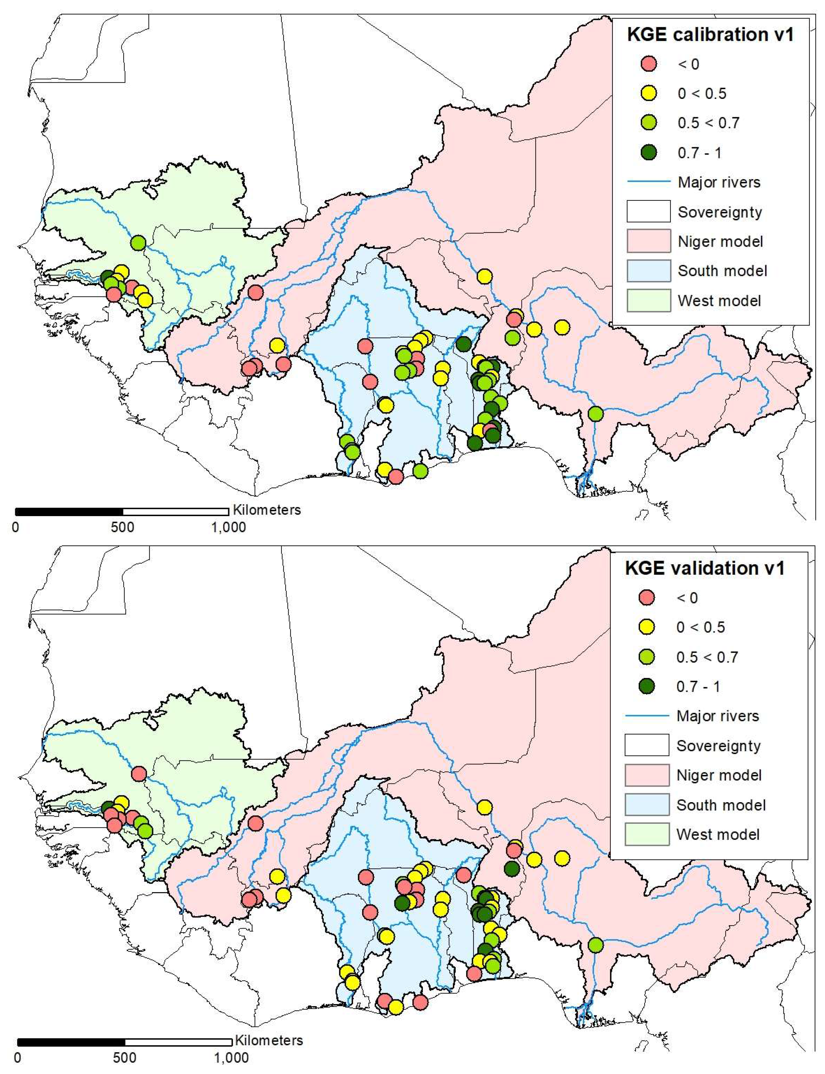
For the v1 calibration (Figure 3), 78% of gauging stations reach a KGE of higher than zero, meaning that the model performs better than if using observed mean values as predictors [77]. On average, 40% of the gauging stations reach a KGE of more than 0.5, while 13% are above 0.7, with the highest average KGE of 0.40 in the West (the overall best result) and the lowest average KGE of 0.14 found in the Niger region. The average bias is 14.36% and R2 amounts to 0.52, with the highest R2 of 0.57 reached in the West model and the lowest value of 0.46 in the Niger model. While the range of the model uncertainty (r-Factor) is 0.82, the percentage of data bracketed by the 95 PPU (p-Factor) is 47%. Calibrations of the southern model perform best in the Ouémé and White Volta basins and worst in the Black Volta basin. For the western model, best performances can be observed for the downstream Gambia tributary rivers, while some upstream stations perform less well. For the Niger model, the best performance is reached downstream of the confluence of the Benue and the Niger in Lokoja, while it performs worst in most of the most upstream sub-basins.
Concerning validation, 33% of v1 stations reach a KGE above 0.5 and 12% above 0.7. However, the average KGE is 0.07 due to some poorly-performing stations. If we removed these stations, KGE would increase to 0.42. R2 is the only factor performing better in the validation than the calibration (0.63 as opposed to 0.52). While the p-factor is similar to the calibration, the r-factor is influenced by the large uncertainty band of the West model and reaches 4.41. PBIAS has also increased to 17.59%. Best performances are reached in the West model.
While for the v2 approach (Figure 4), about the same amount of stations score a KGE of higher than 0.5 (73%), it generally delivers less robust solutions, with only 32% of discharge stations reaching a KGE of 0.5 or higher and 10% reaching above 0.7, as opposed to 13% in v1. The average KGE value of simulation v2 is worse in the South (0.15) and Niger (0.08) models and decidedly worse in the West (−0.13). While p and r perform slightly worse in the v2 approach, R2 remains almost constant at 0.51. PBIAS is worse in v2, dropping from 14.36% underestimation to −23.74% overestimation of streamflow. The Comoé, as well as certain upstream Niger basins, perform better. The v2 validation performs worse than the v1 validation, with 25% of stations reaching KGE values above 0.5 and 1% above 0.7. The average KGE is low with −2.94, due to bad performance in the West model. When only taking stations performing above zero into account, KGE is higher with 0.45 than in the v1 validations (0.42). The highest KGE is reached in the Niger (0.10). While the r value for v2 is decidedly better (0.78 as opposed to 4.41), p is slightly worse (0.32 vs. 0.46). v2 strongly overestimates streamflow (PBIAS: −285.95), again mainly due to the performance of the West model. R2 performs similar to v1. Best validation results are reached in the White Volta, Oti and Ouémé.
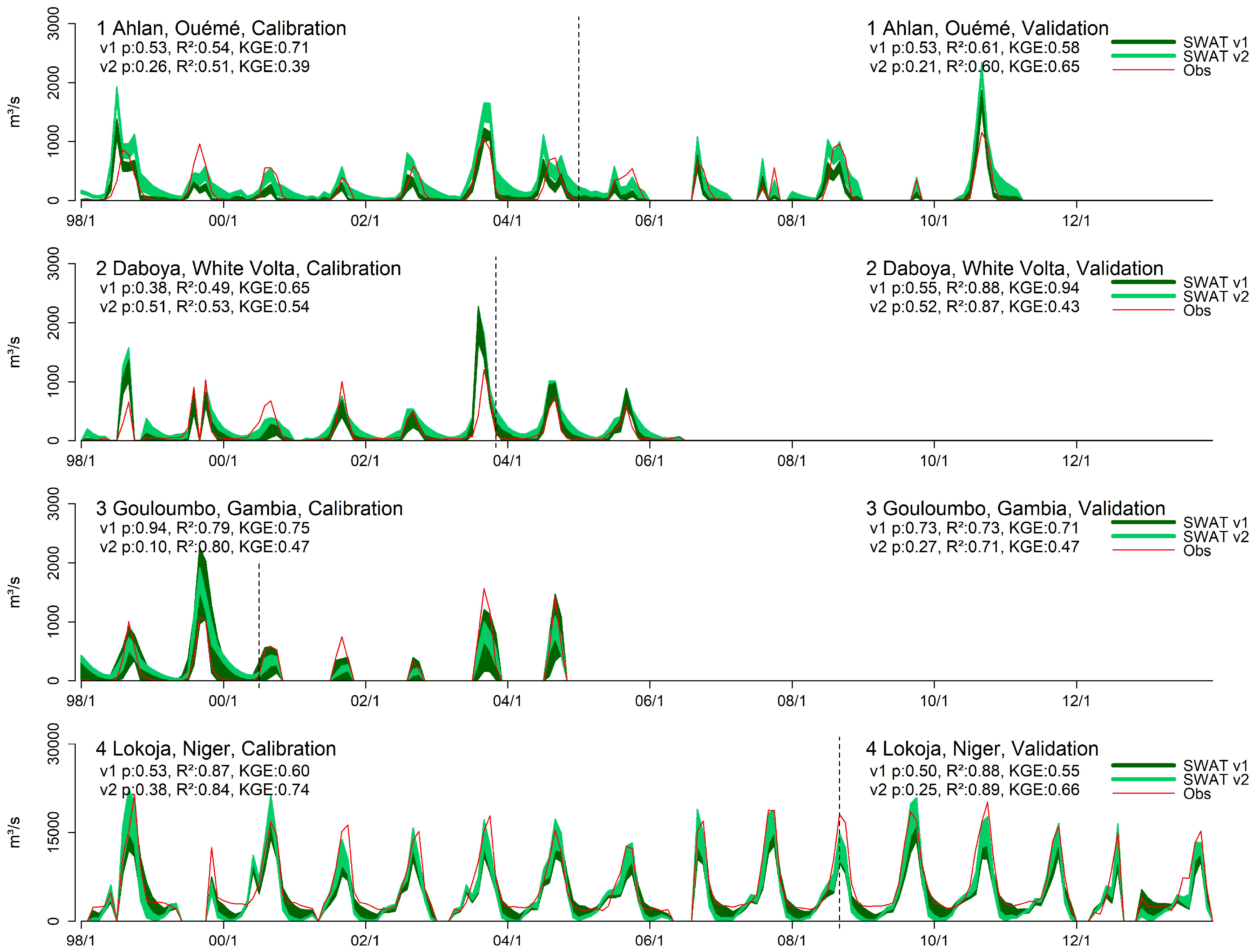
An example of monthly calibration and validation results for four selected discharge stations is given in Figure 5. Displayed are the 95PPU ranges of both v1 and v2 calibration and validation, the observed data, as well as the key efficiency criteria p, R2 and KGE. The stations are located in the Ouémé (1 Ahlan), White Volta (2 Daboya), Gambia (3 Gouloumbo) and Niger (4 Lokoja) river basins. For v1, KGE values for all stations are between 0.65 and 0.75. On average, validations perform less well than calibrations except in Daboya (Validation: 0.94). While performances increase during v2 in Lokoja, decreases can be observed for the other stations. Only during validation do Ahlan and Lokoja perform better than v1. At this point, we conclude that for the calibration and validation of the model with discharge alone, the global calibration (v1) performed slightly better than the local calibration (v2).
3.2. Multi-Objective Validation Results
During the multi-objective validation, several output variables which were not used for calibration were kept for further validation by comparing to MODIS ETa, ESA CCI SM and GRACE data.
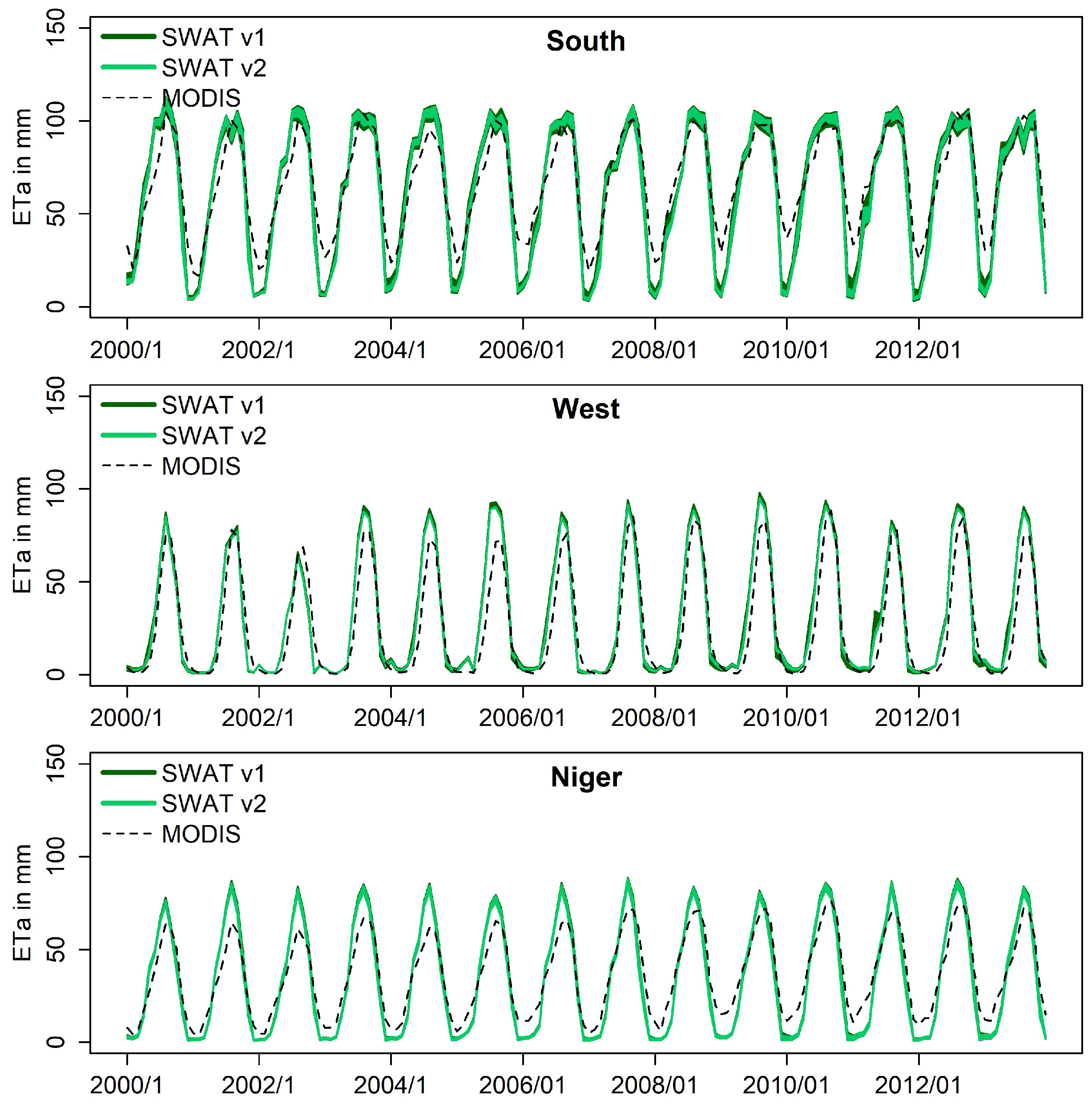
Concerning actual evapotranspiration, validation results reach good scores, as shown in Table 4 and Figure 6.
Both the v1 and v2 calibrations of all models fit the observed data very well, with all criteria being almost identical. Best R2 performances are observed in the Niger model with 0.94. No model R2 performs below 0.91. In both the West and the Niger models, SWAT overestimates ETa during the wet seasons. In the South and Niger models, underestimations during the dry season also occur. On average, the South and Niger model underestimate ETa (PBIAS: −2.8–−6.6%), while the West model overestimates by around 15%. In the West model, no underestimations can be observed due to observed ETa being very low during the dry season.
Performance metrics for the soil moisture validation against ESA CCI data are given in Table 5 and graphical representations in Figure 7.
Overall, the dynamics fit very well. Years with lower soil moisture content such as 2002–2003 in the West, or 2001–2003 in the South model regions are also well represented in the simulations. R2 values are above 0.69 for all models with best performances reached in South v2 and Niger v1/v2 (0.82 and 0.80). West v1 performed least well with an R2 of 0.69. v1 and v2 again perform very similarly (v1: 0.75, v2: 0.78).
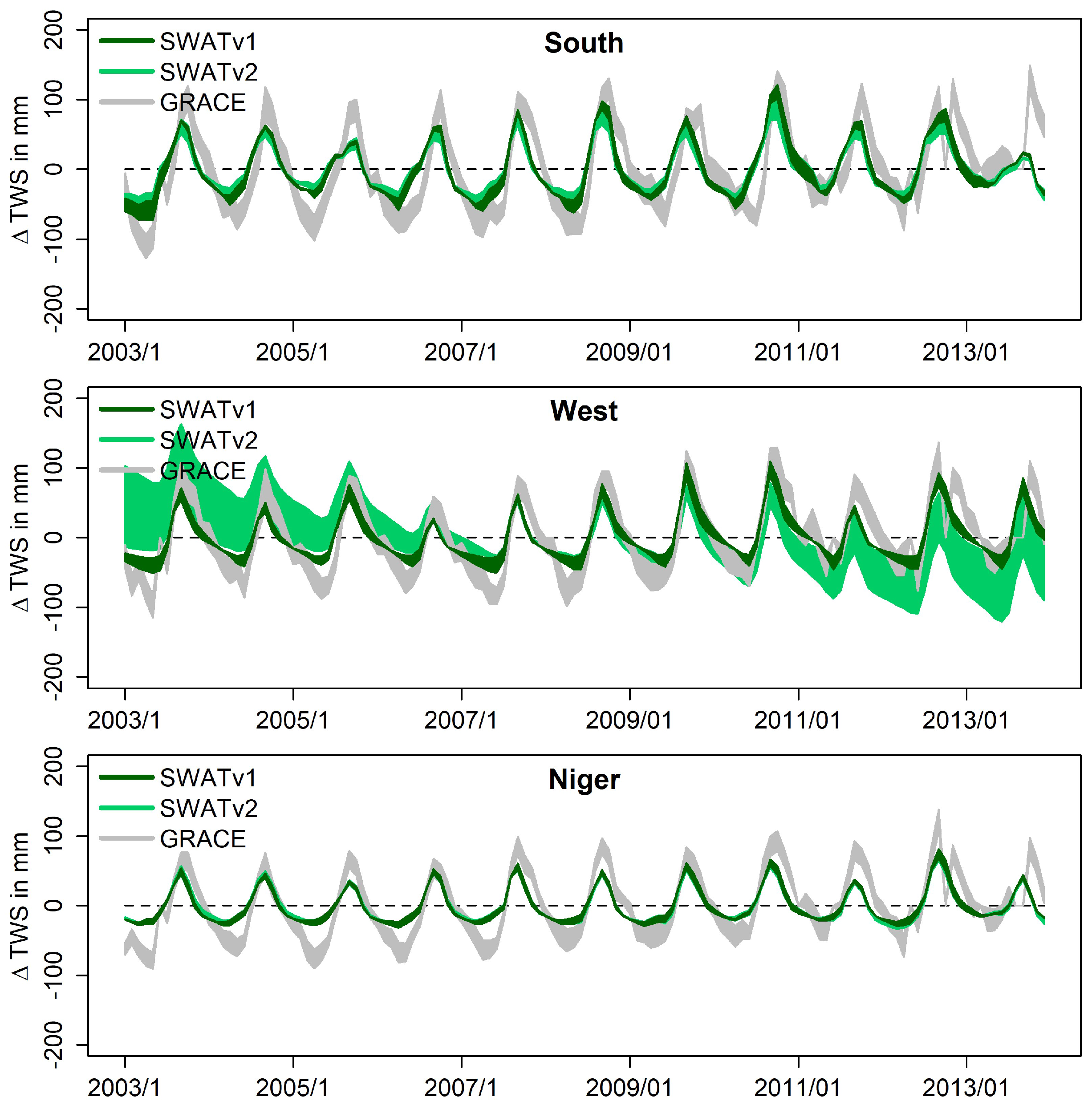
Finally, total water storage was calculated from SWAT outputs and validated using GRACE data (see Table 6 and Figure 8). Again, results show a good fit. Nonetheless, an overestimation of TWS during the dry seasons is apparent in all models, as well as a slight underestimation during the wet seasons in the Niger and South models. Also apparent is a phase shift in the model results by approximately half a month. Some fast changes, e.g., the sharp drop and rise in TWS during the wet season 2012, are not visible in the simulation results at all. Performances vary, and a very high uncertainty in the West v2 model is immediately apparent. Otherwise, the dynamics of both calibrations perform similarly with best R2 and NSE results reached in the globally calibrated models (0.82 and 0.79 as opposed to 0.61 and 0.56 in the locally calibrated models, respectively). All models except West v2 reach between acceptable and very good R2 and NSE values with the West v1 model performing best and the West v2 model performing worst.
4. Discussion
4.1. Model Calibration/Validation Discussion
Results show that satellite and remote sensing data can be used to substitute missing observations and boundary conditions in a SWAT simulation. Results are promising with especially successful calibrations and validations generated for the Ouémé, Gambia and lower Niger basins. It may be argued that during global calibration (v1), a prevalence of stations in a certain region may unduly influence the model if the weights of the stations remain the same [36]. In our case, this can be observed in the Niger basin, where two of the most upstream stations perform poorly due to the calibration being influenced by the downstream gauging stations but performing better when separately calibrated in v2. However, this effect does not explain the poor performance along the Black Volta river, as similarly poor results are observed in the v2 simulation. This was also reported by Schuol et al. [1]. Some of the discharge stations are highly influenced by upstream reservoirs for which no outflow data is available. Even when including reservoirs in the SWAT model, we noticed downstream stations often performed poorly due to the limited amount of data available for proper reservoir setup. Also problematic is the decline in the availability of discharge measurements and uncertainty as to their quality, coupled with data gaps. In contrast to Schuol et al. [1], we did not include the Inner Niger Delta in the model. While they set up the delta as an artificial reservoir and defined the outflow as according to a close downstream station, the closest station for our timeframe is located almost 500 km downstream.
Also, the Akosombo dam in southern Ghana, which creates Lake Volta, could not be included due to missing information about in- and outflows. While the lake was removed from GRACE-derived water storage change (by deriving mass variations using altimeter measurements and information on the lake area) to correspond to the simulations, the missing lake might lead to lower actual evapotranspiration simulations in this area. If comparing the amount of discharge data available for the period modeled by Schuol et al. (calibration from 1970 to 1995) and this study (1998–2013), the decline in available discharge measurements becomes apparent, with the exception of the Ouémé basin, where we were able to secure additional stations. Interestingly, the distribution of well-performing stations is very similar in results from both studies, except for the upstream Niger stations, which performed less well in our approach. We observed v1 performing stronger in the calibration and validation periods. We attribute this to the global sensitivity evaluation used in this study. While the 500 runs used to evaluate the sensitivity of the global calibration seem appropriate, we believe 1000 runs for the local sensitivity analysis might have been too low, especially considering the large number of parameters used, which influences the relative sensitivity of each parameter [84]. While [84] suggest between 500 and 1000 runs suffice, we believe the effects of more runs especially when using many parameters should be studied. Opening the parameter ranges further might lead to increased p-values and better calibrations/validations. However, effects of the parameters on hydrological processes not represented in the streamflow must be carefully assessed. We encountered several difficulties with unrealistic soil moisture and aquifer behavior using less restricted ranges, which led to bad multi-objective validation results. Furthermore, it can be assumed that if more stations with longer and more complete time series are available, better and more accurate results can be generated.
4.2. Multi-Objective Validation Discussion
It seems unrealistic to expect more discharge observations becoming available in the near future. So far, discharge measurements based on satellite-derived water levels have been limited to rivers wider than about 100 m, their spatial coverage is limited by orbit patterns, and they rely on assumptions inherent to rating-curve approaches or river hydraulic modeling which are difficult to verify. Therefore, alternative methods for verifying the accuracy of hydrological model outputs must be explored [82]. The multi-objective validation allows us to assess the performance of the model for multiple aspects of the water balance. In terms of actual evapotranspiration, the remote sensing and reanalysis climate forcings allowed for a very good performance at the basin scale.
When looking at single sub-basins, however, the model tends to overpredict ETa in extremely arid areas. In some very humid sub-basins, ETa may likewise be underpredicted. When validating MOD 16 ETa for South Africa, underpredictions of between 13% and 35% have been found [85,86], leading us to assume that the apparent overestimation in arid areas in our model may in part be due to inaccuracies of the MODIS validation data, while the underestimation of ETa during the dry seasons in the southern model could be explained due to Lake Volta not being simulated.
Dynamics of the modeled soil moisture fit the observations very well. The SWAT uncertainties increase markedly during the wet seasons due to a higher availability of water and thus greater influence of the governing parameters. SWAT SM outputs do not allow for a direct comparison, due to the lack of residual water content included in the results.
The validation of the simulated total water storage with GRACE showed good agreement with some peculiarities. The phase shift of one-half month that we identify, especially in the South and West models, has also been observed by Grippa et al. [87] and Ndehedehe et al. [88] when comparing multi-model results with GRACE solutions for West Africa. The most noticeable difference between model and GRACE solutions is the very pronounced decline in TWS during the dry season retrieved by GRACE, which is not always captured by SWAT. This discrepancy is very strong in the West and Niger models, and while it may in part be due to our calculation of the TWS change in SWAT, similar observations have been reported in other studies. Grippa et al. compared water storage anomalies derived from nine land surface models to GRACE, both for the Sahel and West Africa [87]. Their findings are very similar to ours, with SWAT TWS change estimations of our West model comparing well to the Sahel zone and the South model to the West Africa zone, while the Niger model lies in between the two. They assume that incorrectly modeled evapotranspiration during the dry season led to these results. Boone et al. [89] also compared land-surface models (LSMs) with GRACE over West Africa and came to the conclusion that the difference in amplitudes might either be due to deficits in the precipitation forcing of the LSMs, their insufficient soil depth (where water percolating past a certain depth is lost, similar to SWAT) or the overestimation of the storage anomalies by GRACE during the dry season. Similar observations were made by Ndehedehe et al., 2016, who speculate that differences might be due to anthropogenic influences intensifying land surface processes which the models cannot capture, or the lack of observed data for model calibration leading to improper soil moisture outputs and thus wrong TWS solutions [88]. Werth et al. [90] observed an increase in total water storage over the Niger river basin of seven mm/year and conclude this to be mainly due to an accumulation of groundwater in the Sahel Zone. While we observe positive trends of the total water storage for all models except West v2, which is influenced by high uncertainties, trends in SWAT are generally lower than the GRACE solutions. Furthermore, several studies [20,90,91,92] report a clear positive trend toward a higher total water storage over the Volta basin since 2007 due to increased precipitation. We have seen a similar effect before removing the Lake Volta signal from the GRACE solution, where we observed a trend of 25 mm/year from January 2007 to December 2010. Afterwards, a positive trend is much less evident, and we conclude that their results were masked by the strong signal of the lake.
5. Conclusions
For the first time, to the authors’ knowledge, has a SWAT model been calibrated using remote sensing and reanalysis inputs and validated for streamflow, actual evapotranspiration, soil moisture dynamics and total water storage simultaneously, proving its robustness and predictive capability. Results show that SWAT simulations for different sparsely-gauged regions of West Africa using freely available remote sensing and reanalysis datasets as input perform surprisingly well. This framework significantly eases the modeler’s task of acquiring the necessary climatological, land use and soil data to parameterize a physically-based model. Especially considering the lack of measurements conducted in-situ, the use of remote sensing is essential to produce meaningful assumptions of the water resources in West Africa. While the models perform well using two different calibration and validation schemes, it is necessary to further validate parameters apart from streamflow, otherwise errors in other parts of the water balance might be overlooked. Worqlul et al. have e.g., shown that streamflow may be well simulated even if input precipitation data has large errors [26]. We therefore chose to additionally validate actual evapotranspiration, soil moisture and total water storage outputs. The multi-objective validation produced very good results and confirmed that the model performs well in the study area. While our approach delivers good results at the regional, sub-continental scale, we realize that it might not be appropriate to model smaller catchments. The model framework could be further improved if data becomes available to accurately model the Niger Inland Delta and Lake Volta. Also, the sensitivity analysis procedure should be improved if using a large number of potential parameters, as in our v2 approach. Furthermore, parameters such as actual evapotranspiration or leaf area index could be included in a multi-objective calibration using SWAT-CUP. Our framework offers possibilities for further evaluation of the water cycle in West Africa. In ongoing work, we plan to evaluate the model performance against global hydrological models to investigate capabilities and limitations of these models and investigate the model response to extreme drought and flood events. Also, the performance of SWAT with different remote sensing inputs can be evaluated for the region. Nonetheless, it is the authors’ opinion that remote sensing data should only be used to complement and not replace discharge and other in-situ measurements for model calibration and validation. Despite the availability of satellite measurements, we believe countries should still invest in in-situ measurement networks.
Acknowledgments
This study is part of the COAST project (Studying changes of sea level and water storage for coastal regions in West-Africa using satellite and terrestrial data sets) of the University of Bonn, supported by the Deutsche Forschungsgemeinschaft (German Research Foundation) under Grants No. DI443/6-1 and KU1207/20-1. We are grateful to Christophe Peugeot and the AMMA-Catch project as well as to the Global Runoff Data Centre in 56068 Koblenz, Germany for providing discharge data. The AMMA-CATCH regional observing system was set up thanks to an incentive funding of the French Ministry of Research that allowed pooling together various preexisting small scale observing setups. The continuity and long term perenity of the measurements are made possible by an undisrupted IRD funding since 1990 and by a continuous CNRS-INSU funding since 2005.
Author Contributions
Bernd Diekkrüger and Thomas Poméon designed the framework of the study. Thomas Poméon performed data preparation and SWAT modeling. Bernd Diekkrüger secured additional discharge data and consulted during the modeling process. Anne Springer performed the computations related to the GRACE data. Annette Eicker and Jürgen Kusche contributed their knowledge about GRACE processing and analysis. All authors contributed to the interpretation of the results and proofreading.
Conflicts of Interest
The authors declare no conflict of interest.
References
- Schuol, J.; Abbaspour, K.C.; Srinivasan, R.; Yang, H. Estimation of freshwater availability in the West African sub-continent using the SWAT hydrologic model. J. Hydrol. 2008, 352, 30–49. [Google Scholar] [CrossRef]
- Hollinger, F.; Staatz, J.M. Agricultural Growth in West Africa Market and Policy Drivers. Avalible online: https://reliefweb.int/report/world/agricultural-growth-west-africa-market-and-policy-drivers (accessed on 9 April 2018).
- Jalloh, A.; Faye, M.D.; Roy-Macauley, H.; Sérémé, P.; Zougmoré, R.; Thomas, T.S.; Nelson, G.C. Overview. In West African Agriculture and Climate Change; Jalloh, A., Nelson, G.C., Thomas, T.S., Zougmoré, R., Roy-Macauley, H., Eds.; International Food Policy Research Institute: Washington, DC, USA, 2013. [Google Scholar]
- Andersen, J.; Refsgaard, J.C.; Jensen, K.H. Distributed hydrological modelling of the Senegal River Basin—Model construction and validation. J. Hydrol. 2001, 247, 200–214. [Google Scholar] [CrossRef]
- Bormann, H. Regional hydrological modelling in Benin (West Africa): Uncertainty issues versus scenarios of expected future environmental change. Phys. Chem. Earth 2005, 30, 472–484. [Google Scholar] [CrossRef]
- Wagner, S.; Kunstmann, H.; Bárdossy, A.; Conrad, C.; Colditz, R.R. Water balance estimation of a poorly gauged catchment in West Africa using dynamically downscaled meteorological fields and remote sensing information. Phys. Chem. Earth 2009, 34, 225–235. [Google Scholar] [CrossRef]
- Fujihara, Y.; Yamamoto, Y.; Tsujimoto, Y.; Sakagami, J. Discharge Simulation in a Data-Scarce Basin Using Reanalysis and Global Precipitation Data: A Case Study of the White Volta Basin. J. Water Resour. Prot. 2014, 1316–1325. [Google Scholar] [CrossRef]
- Döll, P.; Kaspar, F.; Lehner, B. A global hydrological model for deriving water availability indicators: Model tuning and validation. J. Hydrol. 2003, 270, 105–134. [Google Scholar] [CrossRef]
- Li, K.Y.; Coe, M.T.; Ramankutty, N. Investigation of hydrological variability in West Africa using land surface models. J. Clim. 2005, 18, 3173–3188. [Google Scholar] [CrossRef]
- Schuol, J.; Abbaspour, K.C. Calibration and uncertainty issues of a hydrological model (SWAT) applied to West Africa. Adv. Geosci. 2006, 9, 137–143. [Google Scholar] [CrossRef]
- Schuol, J.; Abbaspour, K.C.; Yang, H.; Srinivasan, R.; Zehnder, A.J.B. Modeling blue and green water availability in Africa. Water Resour. Res. 2008, 44, 1–18. [Google Scholar] [CrossRef]
- Xie, H.; Longuevergne, L.; Ringler, C.; Scanlon, B.R. Calibration and evaluation of a semi-distributed watershed model of Sub-Saharan Africa using GRACE data. Hydrol. Earth Syst. Sci. 2012, 16, 3083–3099. [Google Scholar] [CrossRef]
- Schuol, J.; Abbaspour, K.C. Using monthly weather statistics to generate daily data in a SWAT model application to West Africa. Ecol. Model. 2006, 201, 301–311. [Google Scholar] [CrossRef]
- Arnold, J.G.; Srinivasan, R.; Muttiah, R.S.; Williams, J.R. Large area hydrologic modeling and assessment Part 1: Model development. J. Am. Water Resour. Assoc. 1998, 34, 73–89. [Google Scholar] [CrossRef]
- Behrangi, A.; Khakbaz, B.; Jaw, T.C.; AghaKouchak, A.; Hsu, K.; Sorooshian, S. Hydrologic evaluation of satellite precipitation products over a mid-size basin. J. Hydrol. 2011, 397, 225–237. [Google Scholar] [CrossRef]
- Bitew, M.M.; Gebremichael, M. Assessment of satellite rainfall products for streamflow simulation in medium watersheds of the Ethiopian highlands. Hydrol. Earth Syst. Sci. 2011, 15, 1147–1155. [Google Scholar] [CrossRef] [Green Version]
- Koutsouris, A.J.; Chen, D.; Lyon, S.W. Comparing global precipitation data sets in eastern Africa: A case study of Kilombero Valley, Tanzania. Int. J. Climatol. 2016, 36, 2000–2014. [Google Scholar] [CrossRef]
- Adjei, K.A.; Ren, L.; Appiah-Adjei, E.K.; Kankam-Yeboah, K.; Agyapong, A.A. Validation of TRMM Data in the Black Volta Basin of Ghana. J. Hydrol. Eng. 2012, 17, 647–654. [Google Scholar] [CrossRef]
- Hughes, D.A. Comparison of satellite rainfall data with observations from gauging station networks. J. Hydrol. 2006, 327, 399–410. [Google Scholar] [CrossRef]
- Forootan, E.; Kusche, J.; Loth, I.; Schuh, W.D.; Eicker, A.; Awange, J.; Longuevergne, L.; Diekkrüger, B.; Schmidt, M.; Shum, C.K. Multivariate Prediction of Total Water Storage Changes over West Africa from Multi-Satellite Data. Surv. Geophys. 2014, 35, 913–940. [Google Scholar] [CrossRef] [Green Version]
- Thiemig, V.; Rojas, R.; Zambrano-Bigiarini, M.; Levizzani, V.; De Roo, A. Validation of Satellite-Based Precipitation Products Over Sparsely-Gauged African River Basins. J. Hydrometeorol. 2012. [Google Scholar] [CrossRef]
- Gosset, M.; Viarre, J.; Quantin, G.; Alcoba, M. Evaluation of several rainfall products used for hydrological applications over West Africa using two high-resolution gauge networks. Q. J. R. Meteorol. Soc. 2013, 139, 923–940. [Google Scholar] [CrossRef]
- Poméon, T.; Jackisch, D.; Diekkrüger, B. Evaluating the performance of remotely sensed and reanalysed precipitation data over West Africa using HBV light. J. Hydrol. 2017, 547, 222–235. [Google Scholar] [CrossRef]
- Pfeifroth, U.; Trentmann, J.; Fink, A.H.; Ahrens, B. Evaluating satellite-based diurnal cycles of precipitation in the African tropics. J. Appl. Meteorol. Climatol. 2016, 55, 23–39. [Google Scholar] [CrossRef]
- Bitew, M.M.; Gebremichael, M.; Gebremichael, L.T.; Bayissa, Y.A. Evaluation of High-Resolution Satellite Rainfall Products through Streamflow Simulation in a Hydrological Modeling of a Small Mountainous Watershed in Ethiopia. J. Hydrometeorol. 2012, 13, 338–350. [Google Scholar] [CrossRef]
- Worqlul, A.W.; Yen, H.; Collick, A.S.; Tilahun, S.A.; Langan, S.; Steenhuis, T.S. Evaluation of CFSR, TMPA 3B42 and ground-based rainfall data as input for hydrological models, in data-scarce regions: The upper Blue Nile Basin, Ethiopia. Catena 2017, 152, 242–251. [Google Scholar] [CrossRef]
- Worqlul, A.W.; Maathuis, B.; Adem, A.A.; Demissie, S.S.; Langan, S.; Steenhuis, T.S. Comparison of TRMM, MPEG and CFSR rainfall estimation with the ground observed data for the Lake Tana Basin, Ethiopia. Hydrol. Earth Syst. Sci. Discuss. 2014, 11, 8013–8038. [Google Scholar] [CrossRef]
- Pombo, S.; de Oliveira, R.P.; Mendes, A. Validation of remote-sensing precipitation products for Angola. Meteorol. Appl. 2015, 22, 395–409. [Google Scholar] [CrossRef]
- Awange, J.L.; Ferreira, V.G.; Forootan, E.; Khandu; Andam-Akorful, S.A.; Agutu, N.O.; He, X.F. Uncertainties in remotely sensed precipitation data over Africa. Int. J. Climatol. 2016, 36, 303–323. [Google Scholar] [CrossRef]
- Cotillon, S.E.; Tappan, G.G. Landscapes of West Africa—A Window on a Changing World; U.S. Geological Survey EROS: Garretson, SD, USA, 2016.
- Fink, A.H.; Christoph, M.; Born, K.; Bruecher, T.; Piecha, K.; Pohle, S.; Schulz, O.; Ermert, V. Climate. In Impacts of Global Change on the Hydrological Cycle in West and Northwest Africa; Speth, P., Christoph, M., Diekkrüger, B., Eds.; Springer: Heidelberg, Germany, 2010; pp. 54–58. [Google Scholar]
- Sebastian, K. Agro-Ecological Zones of Africa; International Food Policy Research Institute: Washington, DC, USA, 2009. [Google Scholar]
- Gessner, U.; Niklaus, M.; Kuenzer, C.; Dech, S. Intercomparison of Leaf Area Index Products for a Gradient of Sub-Humid to Arid Environments in West Africa. Remote Sens. 2013, 5, 1235–1257. [Google Scholar] [CrossRef] [Green Version]
- Arnold, J.G.; Moriasi, D.N.; Gassman, P.W.; Abbaspour, K.C.; White, M.J.; Srinivasan, R.; Santhi, C.; Harmel, R.D.; van Griensven, A.; VanLiew, M.W.; et al. SWAT: Model Use, Calibration, and Validation. Trans. ASABE 2012, 55, 1491–1508. [Google Scholar] [CrossRef]
- Srinivasan, R.; Ramanarayanan, T.S.; Arnold, J.G.; Bednarz, S.T. Large area hydrologic modeling and assessment part II: Model application. J. Am. Water Resour. Assoc. 1998, 34, 91–101. [Google Scholar] [CrossRef]
- Abbaspour, K.C.; Rouholahnejad, E.; Vaghefi, S.; Srinivasan, R.; Yang, H.; Kløve, B. A continental-scale hydrology and water quality model for Europe : Calibration and uncertainty of a high-resolution large-scale SWAT model. J. Hydrol. 2015, 524, 733–752. [Google Scholar] [CrossRef]
- Lehner, B.; Verdin, K.; Jarvis, A. HydroSHEDS Technical Documentation Version 1.2; World Wildlife Fund US: Washington, DC, USA, 2013. [Google Scholar]
- Lehner, B.; Verdin, K.; Jarvis, A. New global hydrography derived from spaceborne elevation data. Eos (Washington DC) 2008, 89, 93–94. [Google Scholar] [CrossRef]
- Bontemps, S.; Defourny, P.; Van Bogaert, E.; Arino, O.; Kalogirou, V.; Perez, J. GLOBCOVER 2009 Products Description and Validation Report; Université Catholique de Louvain: Louvain, Belgium; European Space Agency: Paris, France, 2011. [Google Scholar]
- Neitsch, S.; Arnold, J.; Kiniry, J.; Williams, J. Soil & Water Assessment Tool Theoretical Documentation Version 2009; Texas Water Resources Institute: College Station, TX, USA, 2011. [Google Scholar]
- Alemayehu, T.; van Griensven, A.; Bauwens, W. Improved SWAT vegetation growth module for tropical ecosystem. Hydrol. Earth Syst. Sci. Discuss. 2017. [Google Scholar] [CrossRef]
- Strauch, M.; Volk, M. SWAT plant growth modification for improved modeling of perennial vegetation in the tropics. Ecol. Model. 2013, 269, 98–112. [Google Scholar] [CrossRef]
- Myneni, R.; Knyazikhin, Y.; Park, T. MOD15A2H MODIS/Terra Leaf Area Index/FPAR 8-Day L4 Global 500m SIN Grid V006 [LAI 500m]; NASA EOSDIS Land Processes DAAC. Available online: https://doi.org/10.5067/MODIS/MOD15A2H.006 (accessed on 9 April 2018).
- FAO/IIASA/ISRIC/ISS-CAS/JRC. Harmonized World Soil Database (Version 1.2); FAO: Rome, Italy; IIASA: Laxenburg, Austria, 2012; Available online: http://www.fao.org/3/a-aq361e.pdf (accessed on 15 March 2018).
- Wösten, J.H.M.; Pachepsky, Y.A.; Rawls, W.J. Pedotransfer functions: Bridging the gap between available basic soil data and missing soil hydraulic characteristics. J. Hydrol. 2001, 251, 123–150. [Google Scholar] [CrossRef]
- Faramarzi, M.; Abbaspour, K.C.; Ashraf Vaghefi, S.; Farzaneh, M.R.; Zehnder, A.J.B.; Srinivasan, R.; Yang, H. Modeling impacts of climate change on freshwater availability in Africa. J. Hydrol. 2013, 480, 85–101. [Google Scholar] [CrossRef]
- Faramarzi, M.; Abbaspour, K.C.; Schulin, R.; Yang, H. Modelling blue and green water resources availibility in Iran. Hydrol. Process. 2010, 23, 486–501. [Google Scholar] [CrossRef]
- Malagò, A.; Efstathiou, D.; Bouraoui, F.; Nikolaidis, N.P.; Franchini, M.; Bidoglio, G.; Kritsotakis, M. Regional scale hydrologic modeling of a karst-dominant geomorphology: The case study of the Island of Crete. J. Hydrol. 2016, 540, 64–81. [Google Scholar] [CrossRef]
- Joyce, R.J.; Janowiak, J.E.; Arkin, P.A.; Xie, P. CMORPH: A Method that Produces Global Precipitation Estimates from Passive Microwave and Infrared Data at High Spatial and Temporal Resolution. J. Hydrometeorol. 2004, 5, 487–503. [Google Scholar] [CrossRef]
- Xie, P.; Yoo, S.; Joyce, R.; Yarosh, Y. Bias-Corrected CMORPH: A 13-Year Analysis of High-Resolution Global Precipitation. Available online: http://ftp.cpc.ncep.noaa.gov/precip/CMORPH_V1.0/REF/EGU_1104_Xie_bias-CMORPH.pdf (accessed on 13 March 2018).
- Bosilovich, M.G.; Lucchesi, R.; Suarez, M. MERRA-2: File Specification. GMAO Office Note No. 9 (Version 1.1); NASA Goddard Space Flight Center: Greenbelt, MD, USA, 2016.
- Saha, S.; Moorthi, S.; Pan, H.L.; Wu, X.; Wang, J.; Nadiga, S.; Tripp, P.; Kistler, R.; Woollen, J.; Behringer, D.; et al. The NCEP climate forecast system reanalysis. Bull. Am. Meteorol. Soc. 2010, 91, 1015–1057. [Google Scholar] [CrossRef]
- Lehner, B.; Liermann, C.R.; Revenga, C.; Vörösmarty, C.; Fekete, B.; Crouzet, P.; Döll, P.; Endejan, M.; Frenken, K.; Magome, J.; et al. High-resolution mapping of the world’ s reservoirs and dams for sustainable river-flow management. Front. Ecol. Environ. 2011, 9, 494–502. [Google Scholar] [CrossRef]
- Mu, Q.; Zhao, M.; Running, S.W. Improvements to a MODIS global terrestrial evapotranspiration algorithm. Remote Sens. Environ. 2011, 115, 1781–1800. [Google Scholar] [CrossRef]
- Mu, Q.; Heinsch, F.; Zhao, M.; Running, S. Development of a global evapotranspiration algorithm based on MODIS and global meteorology data. Remote Sens. Environ. 2007, 106, 285–304. [Google Scholar] [CrossRef]
- Liu, Y.Y.; Dorigo, W.A.; Parinussa, R.M.; De Jeu, R.A.M.; Wagner, W.; McCabe, M.F.; Evans, J.P.; Van Dijk, A.I.J.M. Trend-preserving blending of passive and active microwave soil moisture retrievals. Remote Sens. Environ. 2012, 123, 280–297. [Google Scholar] [CrossRef]
- Liu, Y.Y.; Parinussa, R.M.; Dorigo, W.A.; De Jeu, R.A.M.; Wagner, W.; Van Dijk, A.I.J.; McCabe, M.F.; Evans, J.P. Developing an improved soil moisture dataset by blending passive and active microwave satellite-based retrievals. Hydrol. Earth Syst. Sci. 2011, 15, 425–436. [Google Scholar] [CrossRef] [Green Version]
- Wagner, W.; Dorigo, W.; de Jeu, R.; Fernandez, D.; Benveniste, J.; Haas, E.; Ertl, M. Fusion of Active and Passive Microwave Observations to Create an Essential Climate Variable Data Record on Soil Moisture. ISPRS Ann. Photogramm. Remote Sens. Spat. Inf. Sci. 2012, 1–7, 315–321. [Google Scholar] [CrossRef]
- Wahr, J.; Molenaar, M.; Bryan, F. Time variability of the Earth’s gravity field’ Hydrological and oceanic effects and their possible detection using GRACE. J. Geophys. Res. 1998, 103, 30205–30229. [Google Scholar] [CrossRef]
- Rietbroek, R.; Fritsche, M.; Brunnabend, S.E.; Daras, I.; Kusche, J.; Schröter, J.; Flechtner, F.; Dietrich, R. Global surface mass from a new combination of GRACE, modelled OBP and reprocessed GPS data. J. Geodyn. 2012, 59–60, 64–71. [Google Scholar] [CrossRef]
- Rietbroek, R.; Brunnabend, S.E.; Kusche, J.; Schröter, J. Resolving sea level contributions by identifying fingerprints in time-variable gravity and altimetry. J. Geodyn. 2012, 59–60, 72–81. [Google Scholar] [CrossRef]
- Cheng, M.; Tapley, B.D.; Ries, J.C. Deceleration in the Earth’s oblateness. J. Geophys. Res. Solid Earth 2013, 118, 740–747. [Google Scholar] [CrossRef]
- Kusche, J. Approximate decorrelation and non-isotropic smoothing of time-variable GRACE-type gravity field models. J. Geodesy 2007, 81, 733–749. [Google Scholar] [CrossRef]
- Long, D.; Longuevergne, L.; Scanlon, B.R. Global analysis of approaches for deriving total water storage changes fromGRACE satellites. Water Resour. Res. 2015, 51, 2574–2594. [Google Scholar] [CrossRef]
- Longuevergne, L.; Scanlon, B.R.; Wilson, C.R. GRACE hydrological estimates for small basins: Evaluating processing approaches on the High Plains aquifer, USA. Water Resour. Res. 2010, 46, 1–15. [Google Scholar] [CrossRef]
- Tanaka, M.; Adjadeh, T.A.; Tanaka, S.; Sugimura, T. Water surface area measurement of Lake Volta using SSM/I 37-GHz polarization difference in rainy season. Adv. Space Res. 2002, 30, 2501–2504. [Google Scholar] [CrossRef]
- Uebbing, B.; Kusche, J.; Forootan, E. Waveform Retracking for Improving Level Estimations From TOPEX/Poseidon, Jason-1, and Jason-2 Altimetry Observations Over African Lakes. IEEE Trans. Geosci. Remote Sens. 2015, 53, 2211–2224. [Google Scholar] [CrossRef]
- Winchell, M.; Srinivasan, R.; Di Luzio, M.; Arnold, J. ArcSWAT Interface for SWAT 2009; USDA Agricultural Research Service: Temple, TX, USA, 2010.
- Itiveh, K.; Bigg, G. The variation of discharge entering the Niger Delta system, 1951–2000, and estimates of change under global warming. Int. J. Climatol. 2008, 28, 659–666. [Google Scholar] [CrossRef]
- Hargreaves, G.H.; Samani, Z.A. Reference Crop Evapotranspiration from Temperature. Appl. Eng. Agric. 1985, 1, 96–99. [Google Scholar] [CrossRef]
- Droogers, P.; Allen, R.G. Estimating reference evapotranspiration under inaccurate data conditions. Irrig. Drain. Syst. 2002, 16, 33–45. [Google Scholar] [CrossRef]
- Weiß, M.; Menzel, L. A global comparison of four potential evapotranspiration equations and their relevance to stream flow modelling in semi-arid environments. Adv. Geosci 2008, 18, 15–23. [Google Scholar] [CrossRef]
- Abbaspour, K.C.; Vejdani, M.; Haghighat, S.; Yang, J. SWAT-CUP Calibration and Uncertainty Programs for SWAT. In Proceedings of the 4th International SWAT Conference, Delft, The Netherlands, 4–6 July 2007; pp. 1596–1602. [Google Scholar]
- Arnold, J.G.; Kiniry, J.R.; Srinivasan, R.; Williams, J.R.; Haney, E.B.; Neitsch, S.L. Soil & Water Assessment Tool: Input/Output Documentation; Texas Water Resources Institute: College Station, TX, USA, 2012. [Google Scholar]
- Neitsch, S.L.; Arnold, J.G.; Kiniry, J.R.; Srinivasan, R.; Williams, J.R. Soil and Water Assessment Tool User’s Manual; Texas Water Resources Institute: College Station, TX, USA, 2002. [Google Scholar]
- Abbaspour, K.C. SWAT-CUP: SWAT Calibration and Uncertainty Programs—A User Manual; Swiss Federal Institute of Aquatic Science and Technology (EAWAG): Dübendorf, Switzerland, 2015. [Google Scholar]
- Gupta, H.V.; Kling, H.; Yilmaz, K.K.; Martinez, G.F. Decomposition of the mean squared error and NSE performance criteria: Implications for improving hydrological modelling. J. Hydrol. 2009, 377, 80–91. [Google Scholar] [CrossRef]
- Nash, J.E.; Sutcliffe, J.V. River Flow Forecasting through Conceptual Models Part I—A Discussion of Principles. J. Hydrol. 1970, 10, 282–290. [Google Scholar] [CrossRef]
- Moriasi, D.N.; Arnold, J.G.; van Liew, M.W.; Bingner, R.L.; Harmel, R.D.; Veith, T.L. Model evaluation guidelines for systematic quantification of accuracy in watershed simulations. Trans. ASABE 2007, 50, 885–900. [Google Scholar] [CrossRef]
- Qiao, L.; Herrmann, R.B.; Pan, Z. Parameter Uncertainty Reduction for SWAT Using Grace, Streamflow, and Groundwater Table Data for Lower Missouri River Basin. J. Am. Water Resour. Assoc. 2013, 49, 343–358. [Google Scholar] [CrossRef]
- DeLiberty, T.L.; Legates, D.R. Interannual and seasonal variability of modelled soil moisture in Oklahoma. Int. J. Climatol. 2003, 23, 1057–1086. [Google Scholar] [CrossRef]
- Milzow, C.; Krogh, P.E.; Bauer-Gottwein, P. Combining satellite radar altimetry, SAR surface soil moisture and GRACE total storage changes for hydrological model calibration in a large poorly gauged catchment. Hydrol. Earth Syst. Sci. 2011, 15, 1729–1743. [Google Scholar] [CrossRef] [Green Version]
- Rajib, M.A.; Merwade, V.; Yu, Z. Multi-objective calibration of a hydrologic model using spatially distributed remotely sensed/in-situ soil moisture. J. Hydrol. 2016, 536, 192–207. [Google Scholar] [CrossRef]
- Abbaspour, K.; Vaghefi, S.; Srinivasan, R. A Guideline for Successful Calibration and Uncertainty Analysis for Soil and Water Assessment: A Review of Papers from the 2016 International SWAT Conference. Water 2017, 10, 6. [Google Scholar] [CrossRef]
- Jovanovic, N.; Mu, Q.; Bugan, R.D.H.; Zhao, M. Dynamics of MODIS evapotranspiration in South Africa. Water SA 2015, 41, 79–91. [Google Scholar] [CrossRef]
- Sun, Z.; Gebremichael, M.; Ardö, J.; Nickless, A.; Caquet, B.; Merboldh, L.; Kutschi, W. Estimation of daily evapotranspiration over Africa using MODIS/Terra and SEVIRI/MSG data. Atmos. Res. 2012, 112, 35–44. [Google Scholar] [CrossRef]
- Grippa, M.; Kergoat, L.; Frappart, F.; Araud, Q.; Boone, A.; De Rosnay, P.; Lemoine, J.M.; Gascoin, S.; Balsamo, G.; Ottlé, C.; et al. Land water storage variability over West Africa estimated by Gravity Recovery and Climate Experiment (GRACE) and land surface models. Water Resour. Res. 2011, 47, 1–18. [Google Scholar] [CrossRef]
- Ndehedehe, C.; Awange, J.; Agutu, N.; Kuhn, M.; Heck, B. Understanding Changes in Terrestrial Water Storage over West Africa between 2002 and 2014. Adv. Water Resour. 2016, 88, 211–230. [Google Scholar] [CrossRef]
- Boone, A.; Decharme, B.; Guichard, F.; de Rosnay, P.; Balsamo, G.; Beljaars, A.; Chopin, F.; Orgeval, T.; Polcher, J.; Delire, C.; et al. The AMMA Land Surface Model Intercomparison Project (ALMIP). Bull. Am. Meteorol. Soc. 2009, 90, 1865–1880. [Google Scholar] [CrossRef]
- Werth, S.; White, D.; Bliss, D.W. GRACE Detected Rise of Groundwater in the Sahelian Niger River Basin. J. Geophys. Res. Solid Earth 2017. [Google Scholar] [CrossRef]
- Rateb, A.; Kuo, C.-Y.; Imani, M.; Tseng, K.-H.; Lan, W.-H.; Ching, K.-E.; Tseng, T.-P. Terrestrial Water Storage in African Hydrological Regimes Derived from GRACE Mission Data: Intercomparison of Spherical Harmonics, Mass Concentration, and Scalar Slepian Methods. Sensors 2017, 17, 566. [Google Scholar] [CrossRef] [PubMed]
- Hassan, A.; Jin, S. Water storage changes and balances in Africa observed by GRACE and hydrologic models. Geodesy Geodyn. 2016, 7, 39–49. [Google Scholar] [CrossRef]
Figure 1.
Research Area, Soil and Water Assessment Tool (SWAT) Models and Available Discharge Stations.
Figure 1.
Research Area, Soil and Water Assessment Tool (SWAT) Models and Available Discharge Stations.

Figure 2.
Final SWAT Land Use Distribution for each Model, where AGRC: close grown agriculture; AGRL: agriculture; BARR: barren; FRSD: forest deciduous; RNGB: range brush; RNGE: range grasses; WATR: water; WETF: wetlands forested; WETL: wetlands.
Figure 2.
Final SWAT Land Use Distribution for each Model, where AGRC: close grown agriculture; AGRL: agriculture; BARR: barren; FRSD: forest deciduous; RNGB: range brush; RNGE: range grasses; WATR: water; WETF: wetlands forested; WETL: wetlands.

Figure 3.
Calibration and Validation Results of the v1 (Global Calibration) Models.

Figure 4.
Calibration and Validation Results of the v2 (Local Calibration) Models.

Figure 5.
Example Discharge Results for the South (1&2), West (3) and Niger (4) Models.

Figure 6.
Monthly Simulated Actual Evapotranspiration Validation against MODIS MOD 16 Data, where SWAT v1 is the global and v2 the local calibration.
Figure 6.
Monthly Simulated Actual Evapotranspiration Validation against MODIS MOD 16 Data, where SWAT v1 is the global and v2 the local calibration.

Figure 7.
Monthly Simulated Soil Moisture Validation against ESA CCI Data, where SWAT v1 is the global and v2 the local calibration.
Figure 7.
Monthly Simulated Soil Moisture Validation against ESA CCI Data, where SWAT v1 is the global and v2 the local calibration.

Figure 8.
Monthly Simulated Total Water Storage Validation against GRACE Data, where SWAT v1 is the global and v2 the local calibration.
Figure 8.
Monthly Simulated Total Water Storage Validation against GRACE Data, where SWAT v1 is the global and v2 the local calibration.


Table 1.
Selected River Basins and Discharge Gauges in the Study Area.
| River Basin | Area in km2 | Gauges | SWAT Model |
|---|---|---|---|
| Niger | 2,246,220 | 12 | Niger |
| Senegal | 480,289 | 1 | West |
| Volta | 425,133 | 16 | South |
| Comoé | 84,533 | 3 | South |
| Gambia | 78,321 | 8 | West |
| Ouémé | 61,057 | 17 | South |
| Mono | 24,310 | 1 | South |
| Pra | 23,345 | 1 | South |
| Ankobra | 8773 | 1 | South |
| Kouffo | 4122 | 1 | South |
| Ayensu | 1753 | 1 | South |
| TOTAL | 3,437,856 | 62 | All |
Table 2.
Parameters Included in SWAT Model and Initial Ranges.
| SWAT Parameter | Differs By | min | max |
|---|---|---|---|
| CN2 * | Land use | −0.5 | 0.1 |
| SOL_AWC * | Soil Texture | −0.1 | 0.5 |
| SOL_K * | Soil Texture | −0.5 | 0.5 |
| SOL_BD * | Soil Texture | −0.5 | 0.1 |
| EPCO * | −0.3 | 0.3 | |
| ESCO * | Land use | −0.3 | 0.3 |
| GW_DELAY | 0 | 100 | |
| GWQMN | 0 | 1000 | |
| RCHRG_DP | 0 | 1 | |
| GW_REVAP | 0.02 | 0.2 | |
| REVAPMN | 0 | 500 | |
| SURLAG | 0 | 10 |
CN2: runoff curve number; SOL_AWC: available water capacity (mm H2O/mm soil); SOL_K: saturated hydraulic conductivity (mm/h); SOL_BD: moist bulk density (g/cm3); EPCO: plant uptake compensation factor; ESCO: soil evaporation compensation factor; GW_DELAY: groundwater delay time (days); GWQMN: threshold depth for return flow to occur (mm H2O); RCHRG_DP: deep aquifer percolation fraction; GW_REVAP: groundwater “revap” coefficient; REVAPMN: threshold depth for “revap” or percolation to occur (mm H2O); SURLAG: surface runoff lag coefficient; *: relative change.
Table 3.
Calibration and Validation Results for v1 and v2 Models.
| Model | Objective Function | % of Discharge Stations | |||||||
|---|---|---|---|---|---|---|---|---|---|
| p | r | R2 | PBIAS | KGE | KGE ≥ 0 | KGE ≥ 0 | KGE ≥ 0.5 | KGE ≥ 0.7 | |
| Calibration | |||||||||
| South v1 | 0.37 | 0.36 | 0.53 | 5.54 | 0.23 | 0.48 | 85 | 54 | 20 |
| South v2 | 0.31 | 0.71 | 0.51 | −29.71 | 0.15 | 0.47 | 66 | 39 | 5 |
| West v1 | 0.73 | 1.42 | 0.57 | 7.01 | 0.40 | 0.54 | 90 | 50 | 20 |
| West v2 | 0.33 | 0.79 | 0.61 | −53.50 | −0.13 | 0.38 | 78 | 33 | 0 |
| Niger v1 | 0.30 | 0.65 | 0.46 | 30.53 | 0.14 | 0.38 | 58 | 17 | 0 |
| Niger v2 | 0.29 | 0.62 | 0.41 | 11.98 | 0.08 | 0.35 | 75 | 25 | 25 |
| Average v1 | 0.47 | 0.81 | 0.52 | 14.36 | 0.26 | 0.47 | 78 | 40 | 13 |
| Average v2 | 0.31 | 0.71 | 0.51 | −23.74 | 0.03 | 0.40 | 73 | 32 | 10 |
| Validation | |||||||||
| South v1 | 0.36 | 0.44 | 0.61 | −1.39 | 0.03 | 0.48 | 78 | 37 | 17 |
| South v2 | 0.30 | 0.80 | 0.60 | −62.67 | −0.21 | 0.54 | 73 | 49 | 24 |
| West v1 | 0.72 | 12.22 | 0.74 | 20.43 | 0.17 | 0.47 | 67 | 44 | 11 |
| West v2 | 0.30 | 0.97 | 0.71 | −825.36 | −8.72 | 0.32 | 67 | 0 | 0 |
| Niger v1 | 0.30 | 0.57 | 0.52 | 33.73 | 0.03 | 0.30 | 67 | 17 | 8 |
| Niger v2 | 0.36 | 0.59 | 0.53 | 30.18 | 0.10 | 0.48 | 50 | 25 | 8 |
| Average v1 | 0.46 | 4.41 | 0.63 | 17.59 | 0.07 | 0.42 | 70 | 33 | 12 |
| Average v2 | 0.32 | 0.78 | 0.61 | −285.95 | −2.94 | 0.45 | 63 | 25 | 11 |
p: fraction of data bracketed by the 95PPU; r: 95PPU range (dimensionless); R2: coefficient of determination; PBIAS: percent model bias; KGE: Kling-Gupta Efficiency, KGE ≥ 0: mean KGE of stations scoring higher than 0.
Table 4.
Actual Evapotranspiration Validation against MODIS MOD 16 Data.
| Model | R2 | sig. | PBIAS | NSE | KGE |
|---|---|---|---|---|---|
| South v1 | 0.93 | <0.001 | 5.0 | 0.81 | 0.71 |
| South v2 | 0.92 | <0.001 | 6.6 | 0.73 | 0.63 |
| West v1 | 0.92 | <0.001 | −15.8 | 0.88 | 0.80 |
| West v2 | 0.91 | <0.001 | −15.1 | 0.87 | 0.82 |
| Niger v1 | 0.94 | <0.001 | 2.8 | 0.81 | 0.67 |
| Niger v2 | 0.94 | <0.001 | 4.4 | 0.82 | 0.70 |
| Average v1 | 0.93 | 2.67 | 0.83 | 0.73 | |
| Average v2 | 0.92 | 1.37 | 0.81 | 0.72 |
R2: coefficient of determination; sig: significance; PBIAS: percent model bias; NSE: Nash-Sutcliffe Efficiency.
Table 5.
Soil Moisture Validation against ESA CCI Data.
| Model | R2 | sig. |
|---|---|---|
| South v1 | 0.77 | <0.001 |
| South v2 | 0.82 | <0.001 |
| West v1 | 0.69 | <0.001 |
| West v2 | 0.73 | <0.001 |
| Niger v1 | 0.80 | <0.001 |
| Niger v2 | 0.80 | <0.001 |
| Average v1 | 0.75 | |
| Average v2 | 0.78 |
Table 6.
Total Water Storage Validation against GRACE Data.
| Model | R2 | sig. | NSE |
|---|---|---|---|
| South v1 | 0.75 | <0.001 | 0.75 |
| South v2 | 0.70 | <0.001 | 0.68 |
| West v1 | 0.90 | <0.001 | 0.87 |
| West v2 | 0.35 | <0.001 | 0.27 |
| Niger v1 | 0.82 | <0.001 | 0.76 |
| Niger v2 | 0.79 | <0.001 | 0.72 |
| Average v1 | 0.82 | 0.79 | |
| Average v2 | 0.61 | 0.56 |
© 2018 by the authors. Licensee MDPI, Basel, Switzerland. This article is an open access article distributed under the terms and conditions of the Creative Commons Attribution (CC BY) license (http://creativecommons.org/licenses/by/4.0/).
Share and Cite
MDPI and ACS Style
Poméon, T.; Diekkrüger, B.; Springer, A.; Kusche, J.; Eicker, A. Multi-Objective Validation of SWAT for Sparsely-Gauged West African River Basins—A Remote Sensing Approach. Water 2018, 10, 451. https://doi.org/10.3390/w10040451
AMA Style
Poméon T, Diekkrüger B, Springer A, Kusche J, Eicker A. Multi-Objective Validation of SWAT for Sparsely-Gauged West African River Basins—A Remote Sensing Approach. Water. 2018; 10(4):451. https://doi.org/10.3390/w10040451
Chicago/Turabian StylePoméon, Thomas, Bernd Diekkrüger, Anne Springer, Jürgen Kusche, and Annette Eicker. 2018. "Multi-Objective Validation of SWAT for Sparsely-Gauged West African River Basins—A Remote Sensing Approach" Water 10, no. 4: 451. https://doi.org/10.3390/w10040451
Note that from the first issue of 2016, this journal uses article numbers instead of page numbers. See further details here.