Correlation Analysis of Rainstorm Runoff and Density Current in a Canyon-Shaped Source Water Reservoir: Implications for Reservoir Optimal Operation

Abstract

Extreme weather has recently become frequent. Heavy rainfall forms storm runoff, which is usually very turbid and contains a high concentration of organic matter, therefore affecting water quality when it enters reservoirs. The large canyon-shaped Heihe Reservoir is the most important raw water source for the city of Xi’an. During the flood season, storm runoff flows into the reservoir as a density current. We determined the relationship among inflow peak discharge (Q), suspended sediment concentration, inflow water temperature, and undercurrent water density. The relationships between (Q) and inflow suspended sediment concentration (C_S0) could be described by the equation C_S0 = 0.3899 × e^0.0025Q, that between C_S0 and suspended sediment concentration at the entrance of the main reservoir area S1 (C_S1) was determined using C_S1 = 0.0346 × e^0.2335CS0, and air temperature (T_a) and inflow water temperature (T_w) based on the meteorological data were related as follows: T_w = 0.7718 × T_a + 1.0979. Then, we calculated the density of the undercurrent layer. Compared to the vertical water density distribution at S1 before rainfall, the undercurrent elevation was determined based on the principle of equivalent density inflow. Based on our results, we proposed schemes for optimizing water intake selection and flood discharge during the flood season.

1. Introduction

In recent years, reservoirs have increasingly been built as sources of drinking water, with concurrent functions related to irrigation, flood control, and power generation [1,2,3]. With the increasing trend of global warming, extreme weather has been occurring at a greater frequency [4,5,6]. Severe rainfall caused by extreme weather impacts lakes and reservoirs [7,8], where an accumulation of sediment and increase in turbidity often accompany the heavy rainfall [9,10,11]. The sudden increase in suspended sediment and organic matter due to inflow water with high turbidity after rainfall events markedly affects water quality [12,13]. Highly turbid raw water increases the operating cost of water treatment plants [14,15,16]. The input of easily decomposed organic matter can cause a rise in the dissolved oxygen consumption rate and lead to anaerobic conditions in the hypolimnion, consequently resulting in significant water quality deterioration because nutrients and metal substances continue to diffuse into this layer from the sediments [17,18].

Most lakes and reservoirs in tropical and subtropical zones usually become thermally stratified owing to the changes in water density in the vertical plane [19,20]. Thermal stratification is strongly associated with hydrodynamics and plays an important role in aquatic ecosystems [18,21]. Rainfall drives runoff, and in stratified reservoirs, the runoff flows into a layer with an equivalent density and moves within this layer, which is known as the density current [22,23,24]. Density currents are divided into sediment density currents, salinity density currents, and temperature density currents [25]. Sediment density currents and temperature density currents are common in source water reservoirs, with the former carrying serious exogenous pollution [26,27].

There are many studies on the numerical models of density currents, and these contain some useful conclusions [28,29,30,31]. However, heavy rainfall during the flood season results in runoff that forms quickly and rapidly reaches the main reservoir from upstream areas [32,33,34]. This requires a quick response from the reservoir managers. However, it usually takes a long time to get the results of calculations from existing numerical models for density currents, which adversely affects the timely scientific scheduling of reservoirs. Therefore, quick and manoeuvrable schemes need to be developed.

The Heihe Reservoir is the most important raw water source for the city of Xi’an. More than 60% of the annual precipitation in this watershed occurs from July to September [3]. Inflow water with high turbidity increases the risk to drinking water security during the flood season. In this study, we determined the relationships among inflow peak discharge, suspended sediment concentration, inflow water temperature, and undercurrent water density. By calculating the elevation of the undercurrent layer and combining it with the outlet elevations of intake tower and spillway tower, we propose a scheme for optimal operation of the Heihe Reservoir during the flood season. We believe that our scheme could also work as a management strategy for managers of other reservoirs.

2. Materials and Methods

2.1. Study Area

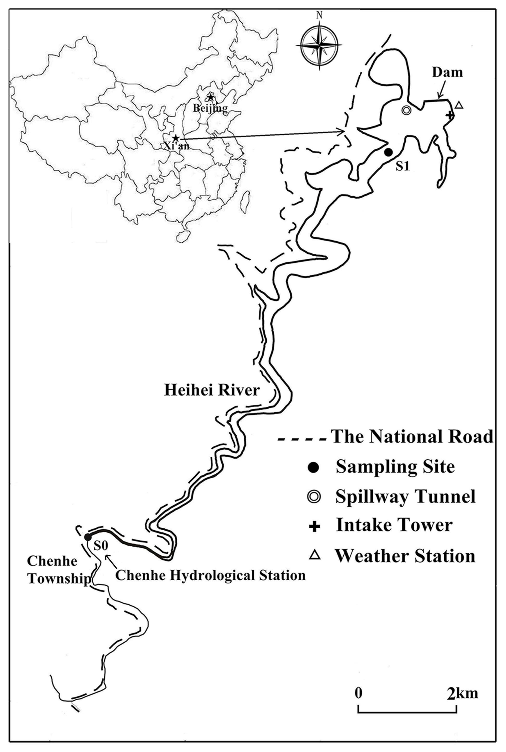
Heihe Reservoir (34°02′24″–34°03′22″ N; 108°11′25″–108°12′33″ E) is a large canyon-shaped reservoir located in Zhouzhi County, approximately 86 km southwest of Xi’an in Shaanxi Province (Figure 1). Xi’an is the capital city of Shaanxi Province and has a population of 8.4 million people. Heihe Reservoir is the most important raw water source for Xi’an, with a daily water supply of 8.0 × 10⁵ m³. When full, the reservoir has a surface area of 4.55 km²; a total capacity of 2.0 × 10⁸ m³; and mean and maximum depths of 44 and 94 m, respectively. Generally, the normal high and minimum water levels are 594 m and 520 m above sea level, respectively. Originating in the Qinling Mountains, the Heihe River, which drains a catchment area of 1481 km², is the main tributary of Heihe Reservoir. The upstream and surrounding landscapes of the reservoir are largely unmodified hills covered by forests that witness little human activity.

2.2. Field Observations

Weekly field sampling campaigns were conducted from 2011 to 2014 to investigate water temperature changes at sampling site S1 (34°02′13.21′′ N 108°11′58.22′′ E). In addition, the suspended sediment (SS) concentration was measured during the flood season. Vertical profiles of water temperature were measured every 2 m from the “surface” (0.5 m below the surface) to the “bottom” (0.5 m above the sediments) at S1 using a Hydrolab DS5X (Hach, Loveland, CO, USA). For the SS concentration, samples were taken every 2 m from the “surface” (0.5 m below the surface) to the “bottom” (0.5 m above the sediments). Sampling site S0 (33°58′34.52′′ N; 108°08′48.96′′ E) was located at the Chenhe hydrological station (at an inlet of the Heihe River) and daily inflow hydrological data, including inflow rate, water temperature, and suspended sediment concentration, was collected there from 2005 to 2014. Daily air temperature was obtained from an automatic weather station near the intake tower. We did not set a sampling site between S1 and S0 because there was no tributary in this area. The input from this area can be ignored compared to that from S0. The maximum runoff flow from the Hanyu River, the tributary on the right side, was about 10 m³/s during the flood season; this is far less than that of the Heihe River. Therefore, we did not discuss it in this study.

3. Results and Discussion

3.1. Variation of Inflow Rate and Suspended Sediment (SS) Concentration

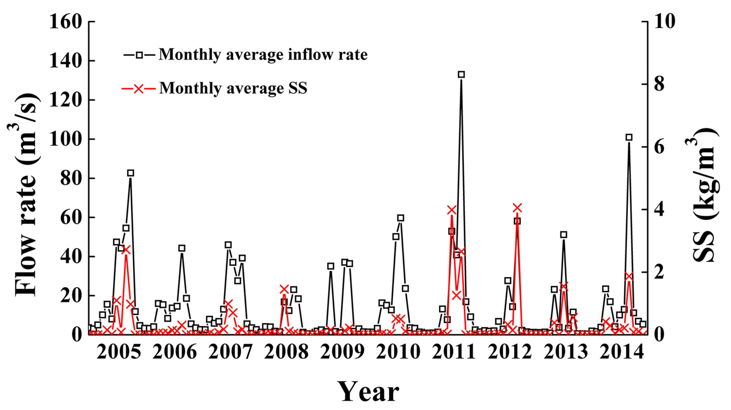
There were large oscillations in the monthly average inflow rate at S0 from 2005 to 2014 (Figure 2). Seasonal rainfall events were influenced by the monsoon climate, and more than 60% of the annual precipitation for the Heihe Reservoir occurred from July to September [3]. This led to a larger monthly average inflow rate from July to September than during other months. There was an obvious change in the monthly average SS concentration as the monthly average inflow rate varied (Figure 2). During the flood season, runoff from both sides of the mountains carried a lot of SS into the Heihe River, thus leading to the rise in SS concentration. At other times, both the monthly average inflow rate and SS concentration were very low.

3.2. Analysis of Peak Discharge and SS Concentration

3.2.1. Relationship between the Inflow Peak Discharge and SS Concentration at S0

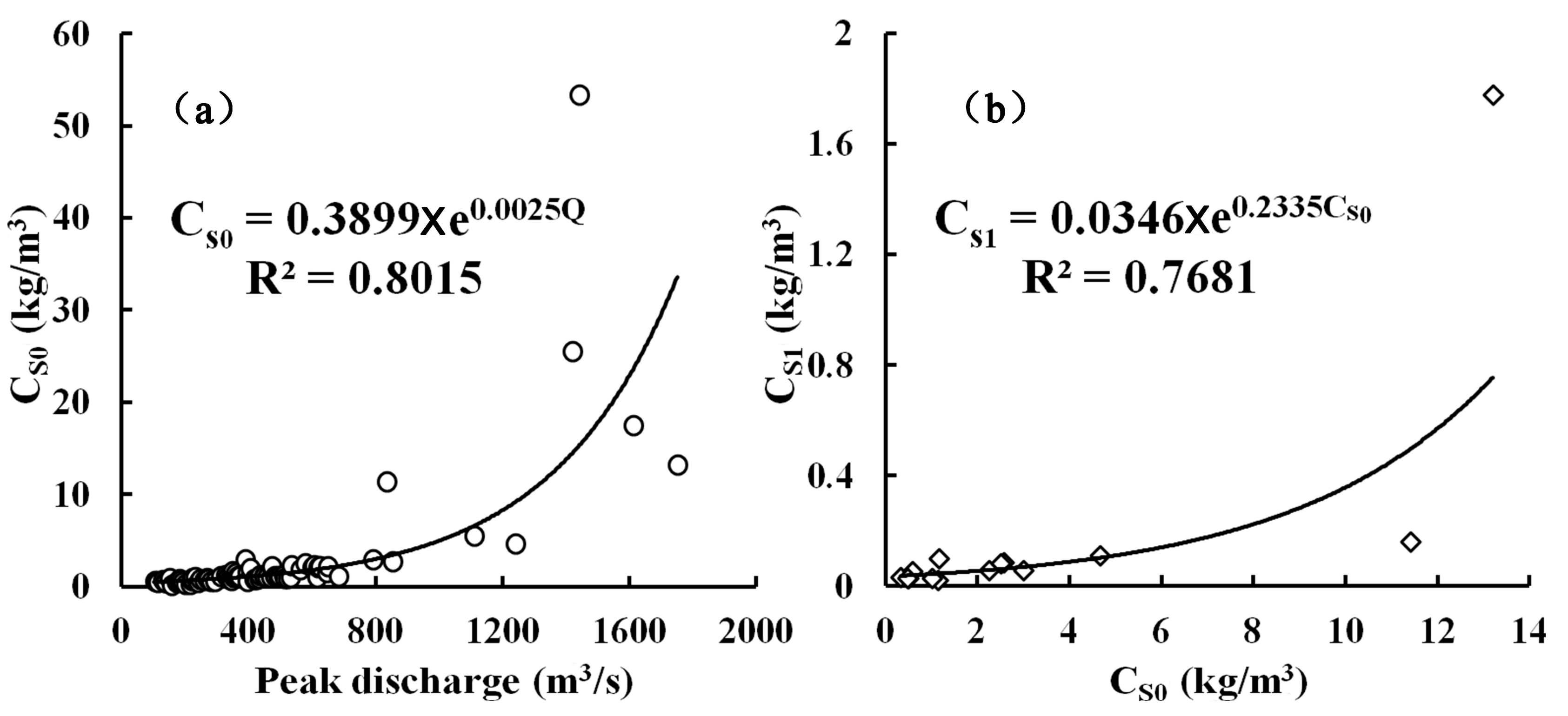
The maximum inflow peak discharge generally corresponded to the maximum SS concentration. However, during the process of runoff formation, the maximum inflow peak discharge was not always consistent with the maximum SS concentration owing to differences in rainfall intensity and concentration of SS in different areas in the Heihe river basin. In this study, we defined an inflow rate above 100 m³/s, which corresponded to the maximum inflow peak discharge with the maximum SS concentration on the same day, as the inflow peak discharge. The relationship between the inflow peak discharge (Q) and SS concentration at S0 (C_S0) is shown in Figure 3a; from this relationship, Formula (1) below is generated:

$${\mathrm{C}}_{\mathrm{S}0}=0.3899\times {\mathrm{e}}^{0.0025\mathrm{Q}},$$

(1)

where Q is in m³/s, and C_S0 is in kg/m³.

Formula (1) was used to calculate the value of C_S0 for different inflow peak discharges. The formula worked better when the inflow peak discharge was less than 1200 m³/s (Figure 3a).

3.2.2. Relationship between SS Concentrations at S0 and at S1

S1 was located at the entrance of the main reservoir area. The water quality at this point reflected the quality of the water that was about to enter the main reservoir area. We monitored the SS concentration at S1 during the flood season from 2011 to 2014 and compared it with that at C_S0 during the same time (

Table 1. Inflow peak discharge and measured inflow suspended sediment concentration (C_S0) at S0, and elevation of undercurrent and measured suspended sediment concentration (C_S1) at S1 from 2011 to 2014.

Date (mm/dd/yy)	S0		S1
	Q (m3/s)	CS0 (kg/m3)	Elevation of Undercurrent (m)	CS1 (kg/m3)
07/10/2011	370	1.141	548	0.025
07/29/2011	1440	53.400	500–520	0.152
09/07/2011	472	2.252	516–530	0.060
09/18/2011	1240	4.655	500–550	0.114
07/09/2012	387	2.991	550	0.060
08/21/2012	190	0.503	553	0.032
09/01/2012	1750	13.207	500–565	1.777
05/26/2013	198	0.324	514	0.034
05/29/2013	497	1.156	530	0.101
07/18/2013	598	2.572	553	0.086
07/23/2013	835	11.402	552	0.161
09/19/2013	230	1.003	525–535	0.031
09/09/2014	576	2.506	527	0.085
09/10/2014	181	1.163	517	0.069
09/12/2014	280	0.581	515–520	0.054
09/17/2014	238	0.467	520	0.031

). C_S1 represents the SS concentration at the undercurrent elevation. For several sets of data (Table 1), the undercurrent elevation fluctuated within a given range. In this case, C_S1 represents the average SS concentration at this range. The peak value of C_S0 reached 53.4 kg/m³ on 29 July 2011, which was significantly higher than other data, indicating that this group of data was not representative. Therefore, it was abandoned when the correlation analysis was performed (Figure 3b). Formula (2) below, in which C_S1 is given in kg/m³, was obtained via data correlation analysis.

$${\mathrm{C}}_{\mathrm{S}1}=0.0346\times {\mathrm{e}}^{{0.2335\mathrm{C}}_{\mathrm{S}0}},$$

(2)

where C_S1 is in kg/m³.

Formula (2) can also be used to calculate the C_S1 for different C_S0 values. The formula worked better when the C_S0 was lower than 6 kg/m³ (Figure 3b). Although the C_S0 were similar on several days (for example, on 07/10/2011 and 09/10/2014, and 08/21/2012 and 09/12/2014 (Table 1)), there were obvious differences in the measured C_S1 value. This was due to the differences in the particle diameter and flow velocity. Generally, particles with a larger diameter result in more obvious sedimentation in the flow process, and different flow velocities change the elevation of undercurrent and thus affect the sedimentation process. It was seen that particle diameter and flow velocity had a very significant influence on the measured results of SS concentration; this was also an important factor that affected the calculation accuracy of Formula (2).

3.3. Analysis of Inflow Water Temperature

3.3.1. Relationship between Inflow Water Temperature and Air Temperature

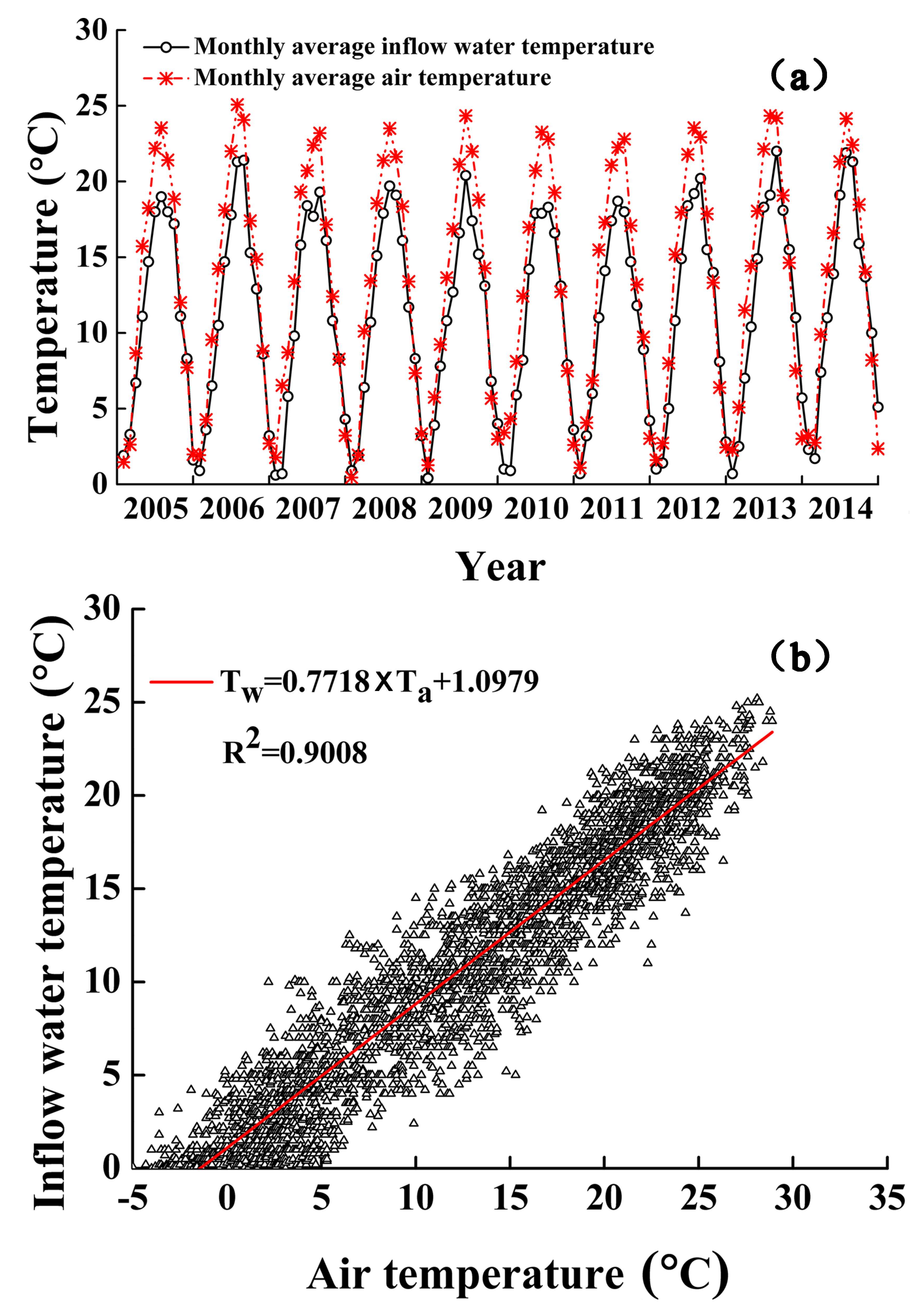
The monthly average inflow water temperature and monthly average air temperature varied between 0.4 °C and 22.0 °C and 0.5 °C and 25.1 °C, respectively; there were obvious amplitudes in both values (Figure 4a). The minimum value of the monthly average inflow water temperature generally occurred in January or February, with the maximum value occurring in July and August every year. From September onwards, the monthly average inflow water temperature and air temperature declined gradually (Figure 4a). The correlation between the inflow water temperature and air temperature was evident; therefore, we could calculate the inflow water temperature using the air temperature.

A linear regression analysis of daily inflow water temperature (T_w) and daily air temperature (T_a) from 2005 to 2014 was conducted (Figure 4b), from which we determined Formula (3) below:

$${\mathrm{T}}_{\mathrm{w}}=0.7718\times {\mathrm{T}}_{\mathrm{a}}+1.0979,$$

(3)

where T_a and T_w are given in °C.

3.3.2. Inflow Water Temperature for Different Inflow Peak Discharges and Months

There were 52 runoff events with an inflow peak discharge over 100 m³/s from 2005 to 2014 (

Table 2. Inflow water temperature for different peak discharges and months from 2005 to 2014.

Month	Date	Peak Discharge	Inflow Water Temperature	Month	Date	Peak Discharge	Inflow Water Temperature
	(mm/dd/yy)	(m3/s)	(°C)		(mm/dd/yy)	(m3/s)	(°C)
May	05/10/2009	164	11.3	Aug.	08/13/2010	304	20.0
	05/26/2013	198	13.0		08/04/2011	371	17.0
	05/25/2012	204	14.3		08/05/2011	390	14.8
	05/14/2009	210	9.5		08/01/2011	435	13.8
	05/29/2013	486	12.8		08/23/2010	509	14.5
Jul.	07/02/2005	151	21.0		08/24/2010	585	13.8
	07/08/2007	192	15.8		08/21/2010	646	16.8
	07/17/2010	198	17.2		08/09/2007	764	17.5
	07/28/2007	248	17.4	Sep.	09/18/2007	139	15.0
	07/07/2012	258	19.0		09/14/2014	150	14.0
	07/05/2007	341	15.5		09/10/2014	181	15.2
	07/10/2011	370	16.3		09/19/2013	230	19.8
	07/31/2011	374	14.2		09/17/2014	238	13.5
	07/09/2012	380	15.6		09/12/2014	280	14.5
	07/23/2010	486	17.6		09/11/2014	290	14.8
	07/18/2013	616	16.5		09/09/2010	290	14.8
	07/21/2008	618	18.5		09/27/2006	293	12.0
	07/24/2010	623	15.0		09/30/2005	356	13.8
	07/18/2005	768	17.0		09/07/2011	472	14.0
	07/23/2013	835	15.8		09/09/2014	576	15.3
	07/29/2011	1430	18.0		09/11/2011	865	14.7
Aug.	08/17/2009	101	19.5		09/18/2011	1240	15.3
	08/31/2007	135	17.0		09/29/2005	1750	13.0
	08/21/2012	190	17.1		09/01/2012	1750	14.8
	08/12/2008	197	18.5	Oct.	10/13/2007	102	9.3
	08/19/2009	267	15.8		10/01/2005	900	13.6

). The rainfall was mainly concentrated in the period from July to September, with a maximum peak discharge of 1750 m³/s (29 September 2005, and 1 September 2012). In May, the inflow water temperature was between 9.5 °C–14.3 °C, with an average value of 12.1 °C. In July, this range was 14.2 °C–21.0 °C, with an average value of 17.0 °C. These were similar to the changes in August, when the temperature ranged from 13.8 °C–20 °C, with an average of 16.5 °C. By September, the inflow water temperature began to decline, varying from 12.0 °C–19.8 °C with an average of 14.6 °C. In October, only two runoff events occurred. In the absence of meteorological data, the inflow water temperature for different inflow peak discharges and months could be roughly estimated using Table 2.

3.4. Calculated Elevation of the Undercurrent

3.4.1. Verification of the Calculated and Measured Results

In a stratified reservoir, the inflow water would flow into a layer with an equivalent density, with water density thought to be primarily determined by water temperature and SS concentration [24]. The water density was calculated via the following formula [35]:

$$\mathrm{D}=1000-1.9549\times {10}^{-2}\times {\left|\mathrm{T}-4\right|}^{1.68}+0.623\times {\mathrm{C}}_{\mathrm{S}},$$

(4)

where D is the water density (kg/m³), T is the water temperature (°C), and C_S is the SS concentration (kg/m³).

The inflow water flowed from S0 to S1 as a density current. When it arrived at S1, the temperature of the undercurrent layer was approximately equal to the inflow water temperature at S0. Therefore, the value of T_w could be used for T in Formula (4). Incorporating Formulas (1) and (2) into Formula (4), we obtained the following:

$$\mathrm{D}=1000-0.019549\times {\left|{\mathrm{T}}_{\mathrm{w}}-4\right|}^{1.68}+0.0216\times {\mathrm{e}}^{0.091\times {\mathrm{e}}^{0.0025\mathrm{Q}}}$$

(5)

The SS concentration was usually very low at S1 before rainfall events occurred. Hence, the SS concentration could be ignored at this time, and the water density of all the vertical layers at S1 could be calculated using the measured water temperature data. Based on Formula (5), we calculated the water density of the undercurrent at S1. According to the principle of equivalent density inflow, the water layer that had the same density before rainfall was the one that the undercurrent flowed into. Thus, the elevation of this layer was the result of the calculation. From 2011 to 2014, 15 typical undercurrent elevations were calculated and compared using the measured data, as shown in

Table 3. Calculated and measured undercurrent elevations.

Date	Peak Discharge	Inflow Water Temperature	CS0	CS1	DS1	CUE	MUE
(mm/dd/yy)	(m3/s)	(°C)	(kg/m3)	(kg/m3)	(kg/m3)	(m)	(m)
07/10/2011	370	16.3	0.983	0.044	998.693	545	548
09/07/2011	472	14.0	1.269	0.047	999.093	520	516–530
09/18/2011	1240	15.3	8.655	0.261	999.014	515	500–550
07/09/2012	380	15.6	1.008	0.044	998.756	543	550
08/21/2012	190	17.1	0.627	0.040	998.439	530	533
09/01/2012	1750	14.8	30.974	47.867	1028.712	500	500–565
05/26/2013	198	13.0	0.640	0.040	999.241	517	514
05/29/2013	497	12.8	1.351	0.047	999.272	535	530
07/18/2013	598	16.5	1.739	0.052	998.671	545	553
07/23/2013	835	15.8	3.144	0.072	998.809	543	552
09/19/2013	230	19.8	0.693	0.041	998.008	538	525–535
09/09/2014	576	15.3	1.646	0.051	998.886	520	527
09/10/2014	181	15.2	0.613	0.040	998.893	513	517
09/12/2014	280	14.5	0.785	0.042	999.007	511	515–520
09/17/2014	238	13.5	0.707	0.041	999.167	510	520

Note: CUE: Calculated undercurrent elevation; MUE: Measured undercurrent elevation.

. There were some errors between the calculated and measured results, but they were generally consistent and the former were able to reflect the undercurrent elevation.

3.4.2. Calculated Undercurrent Elevation for Different Inflow Peak Discharges

Certain features were identified based on the runoff statistics from 2005 to 2014. There were 16 incidents of rainstorm runoff in July and September, and the range of the peak discharges was particularly high. In August, there were 13 incidents of rainstorm runoff and the maximum peak discharge was 764 m³/s, which was less than that in July and September. There were five incidents of rainstorm runoff in May, when the maximum peak discharge was only 486 m³/s. Lastly, since only two incidents of storm runoff occurred in October, the data obtained during this period was not representative of that month. Considering the data in Table 2, we established 15 hypothetical calculation conditions for different months and inflow peak discharges: 250 m³/s and 500 m³/s in May; 250 m³/s, 500 m³/s, 800 m³/s, 1000 m³/s, and 1500 m³/s in July; 250 m³/s, 500 m³/s, and 800 m³/s in August; and 250 m³/s, 500 m³/s, 800 m³/s, 1000 m³/s, and 1500 m³/s in September. These values were used to investigate the change in CUE for different months and inflow peak discharge conditions (

Table 4. Calculated undercurrentelevation (CUE) for different months and peak discharges.

Month	Peak Discharge	Inflow Water Temperature	CS0	CS1	DS1	CUE
	(m3/s)	(°C)	(kg/m3)	(kg/m3)	(kg/m3)	(m)
May	250	12.1	0.728	0.041	999.369	520
	500	11.5	1.361	0.048	999.453	518
Jul.	250	17.4	0.728	0.041	998.496	547
	500	17.6	1.361	0.048	998.461	548
	800	17.0	2.881	0.068	998.588	545
	1000	17.0	4.750	0.105	998.612	544
	1500	18.0	16.579	1.661	999.388	518
Aug.	250	15.8	0.728	0.041	998.790	520
	500	14.5	1.361	0.048	999.014	518
	800	17.5	2.881	0.068	998.493	528
Sep.	250	13.5	0.728	0.041	999.167	508
	500	15.8	1.361	0.048	998.794	520
	800	14.7	2.881	0.068	998.994	515
	1000	12.8	4.750	0.105	999.311	511
	1500	13.0	16.579	1.661	1000.251	500

). We chose the inflow water temperature from the data set that had the inflow peak discharge closest to the hypothetical conditions, and used this as the inflow water temperature for each calculation condition.

The results showed that the CUEs ranged from 518 m to 520 m in May. However, in July, the calculated results were around 546 m, except when the inflow peak discharge was equal to 1500 m³/s. This is mainly because the inflow water temperature was higher in July than in May. In August and September, as the inflow water temperature decreased, the CUEs also decreased, ranging from 500 m to 528 m (Table 4). These results could provide data support for an optimal operation scheme for the Heihe Reservoir during the flood season.

3.5. An Optimal Operation Scheme for the Reservoir during Flood Season

3.5.1. Water Intake Selection Scheme

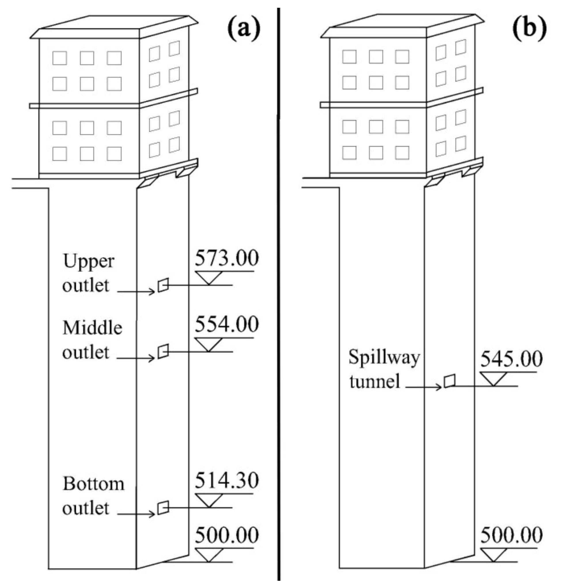
The intake tower of the Heihe Reservoir is located on the right bank of the dam and has upper, middle, and bottom outlets at elevations of 571.0 m, 554.0 m, and 514.3 m, respectively (Figure 5a). During the flood season, the water quality of the reservoir might worsen abruptly and affect the water treatment plant. When storm runoff incidents occur, masses of suspended sediment and humus in the inflow water directly cause effluent quality of the water treatment plant to fall to substandard levels [3].

According to the calculation results in

Table 5. Limiting height of aspiration for different flow rates of flood discharge.

Flow Rate of Flood Discharge (m3/s)	220	506	838	1033
Open height (m)	1.0	2.5	4.0	5.0
Orifice centre elevation (m)	545.5	546.2	547.0	547.50
Limiting height of aspiration (m)	12.5	21.8	30.5	35.1
Lowest elevation of aspiration (m)	533.0	524.4	516.5	512.4

, because the inflow water temperature was low in May, the CUEs were around 520 m. This was close to the height of the bottom outlet. Meanwhile, when the Heihe Reservoir stratified, the quality of the anaerobic water near the bottom outlet was poor [32]. On the other hand, there could be as much as 20 × 10⁶ cells/L of algae in the reservoir in May [36], when the middle outlet might be the best choice; if the algae were not abundant in the surface water, both the upper and middle outlets could be used. In July, the CUEs increased to about 546 m, except for the inflow peak discharge, which was 1500 m³/s; therefore, use of the middle outlet needed to be avoided. If the inflow peak discharge reached 1500 m³/s, the CUE was 518 m; this was close to the elevation of bottom outlet, where the concentration of algae in the surface water could be as high as 30 × 10⁶ cells/L in July and August [36]. Therefore, the bottom and the upper outlet should be closed. Then, when the CUEs decreased to about 500–528 m in August and September, the bottom outlet should be avoided. However, algae were usually rare in September; therefore, the upper or middle outlet could be used at this point.

3.5.2. Flood Discharge Scheme

The spillway tower of the Heihe Reservoir is located on the left bank of the dam, with a bottom elevation of 545 m and a 10 m × 10 m tunnel gate (Figure 5b). As a raw water source reservoir, the inflow SS concentration of the Heihe Reservoir is relatively low for most of the year. Therefore, there is no sediment bore at the bottom of the spillway tower.

In May, the water level was usually low and a high quantity of water was supplied to the city of Xi’an as it was close to summer. Flood discharge would not be carried out at this time despite the occurrence of any runoff. When the Heihe Reservoir began to discharge floodwater, the spillway tunnel gate would be opened, forming an orifice that would suck in a certain thickness of the water layer, half of which was called the limiting height of aspiration. This value could be calculated using the following formula [37]:

$$\mathrm{h}=\mathsf{\phi }*({\mathrm{q}}^2/{\mathsf{\eta }*\mathrm{g})}^{\frac{1}{3}},$$

(6)

where h is the limiting height of aspiration (m), $\mathsf{\phi }$ is a dimensionless coefficient with a value of 0.74, q is the unit width discharge (m³/s), η is the gravity correction coefficient with a value of 0.01, and g is the acceleration due to gravity (m/s²).

The relationship between the flood discharge rate and the open height of the spillway tunnel gate was obtained from the Heihe Reservoir Administration Bureau (Table 5). In July, when the peak discharge was less than 1000 m³/s, the CUEs of around 546 m were close to the elevation of the spillway tunnel (Table 4 and Figure 5b). Opening the gate at that time could discharge highly turbid raw water. When the inflow peak discharge reached 1500 m³/s in July, the CUE dropped to 518 m, which was similar to that in August. If the high turbidity water needed to be discharged, the open height of the gate needed to be at least 4 m. In September, the CUEs dropped to around 510 m, except when the inflow peak discharge was 1500 m³/s; thus, the open height of the gate needed to be greater than 5 m. When the inflow peak discharge was 1500 m³/s or higher, the spillway tunnel did not work; hence, a weir could be set up in front of the spillway tower to raise the CUE. Reservoir managers can use these schemes as scientific management strategies.

3.6. Analysis of Limitation and Application Prospect

The model for calculating the undercurrent elevation in the Heihe Reservoir was established based on a large amount of measured data. It could provide a quick and manoeuvrable technique by which reservoir managers could respond promptly to the occurrence of rainstorm runoff. However, this model also has certain limitations. The relationship between Q and C_S0 worked better when the inflow peak discharge was less than 1200 m³/s; when the inflow peak discharge was higher, the result did not fit very well (Table 3, 09/01/2012). We believe that the neglect of the effects of particle diameter and flow velocity on the sedimentation process was an important reason for this. Furthermore, the inflow water temperature being estimated from the air temperature also led to certain errors in the calculated undercurrent elevation. Despite these errors, the results could still provide a technical scheme for flood discharge and water intake. Moreover, this calculation model is also applicable to other canyon-shaped source water reservoirs although the corresponding correlation analysis should be conducted with data measured from the specific reservoir that the analysis is being applied to. In the future, we aim to do more studies on this issue and establish a model that considers other parameters, such as SS concentration, particle diameter, flow velocity, and water temperature, to calculate the undercurrent elevation. Moreover, we will try to form a visual platform that reservoir managers could use to respond quickly to rainstorm runoff events.

4. Conclusions

(1)

The Heihe Reservoir, a canyon-shaped reservoir in the subtropical zone in northwest China, experiences seasonal rainfall events influenced by a monsoon climate. During the flood season, the SS concentration rises clearly. Based on a correlation analysis of inflow peak discharge (Q) and inflow SS concentration from 2005 to 2014, the relationship between the former and the inflow SS concentration (C_S0) was represented by the formula C_S0 = 0.3899 × e^0.0025Q (R² = 0.8015). Based on a correlation analysis, the inflow SS concentration (C_S0) and the SS concentration at the main area entrance (C_S1) from 2011 to 2014 were found to be related by the equation C_S1 = 0.0346 × e^0.2335C_S0 (R² = 0.7681).

(2)

The inflow water temperature (T_w) and air temperature (T_a) were evidently correlated. The formula we established by correlating the daily data from 2005 to 2014 was T_w = 0.7718 × T_a + 1.0979 (R² = 0.9008). We statistically analysed the inflow water temperature for different inflow peak discharges and months. In the absence of meteorological data, the inflow water temperature could be roughly estimated.

(3)

In the Heihe Reservoir, which is a stratified reservoir, the inflow water flows into a layer of an equivalent density. The undercurrent elevations were calculated and the results were compared with the measured data. The calculated results reflected the undercurrent elevation, showing that the formula used could predict the potential undercurrent elevation in the Heihe Reservoir.

(4)

Fifteen hypothetical calculation conditions, including different months and inflow peak discharges, were established based on the statistics of runoff features from 2005 to 2014. According to the calculation results, a scheme for the optimal operation of reservoirs during the flood season was proposed. In May, the CUEs were approximately 520 m; therefore, if algal blooms occurred during this period, the middle outlet was the best choice for water intake. If the algae concentration in surface water was lower than this, both the upper and middle outlets could be used. When the inflow peak discharge was less than 1000 m³/s in July, the CUEs were close to the height of the spillway tunnel. Opening the spillway tunnel gate could discharge highly turbid water; hence, depending on the concentration of algae during this period, either the upper or the bottom outlet could be used. When the inflow peak discharge reached 1500 m³/s in July, or runoff occurred in August, the CUEs were around 520 m. Therefore, the open height of the spillway tunnel gate needed to be at least 4 m to discharge highly turbid water; therefore, use of the bottom outlet of intake tower should be avoided. In September, when the CUEs were between 500 m and 520 m, the open height of the gate needs to be at least 5 m when the runoff incidents occur; therefore, the use of the bottom outlet of the intake tower should also be avoided at this time.

References

- Kim, H.Y.; Fontane, D.G.; Julien, P.Y.; Lee, J.H. Multiobjective Analysis of the sedimentation behind Sangju Weir, South Korea. J. Water Resour. Plan. Manag. 2018, 144, 05017019. [Google Scholar] [CrossRef]
- Ahmad, A.; El-Shafie, A.; Razali, S.F.M.; Mohamad, Z.S. Reservoir Optimization in Water Resources: A Review. Water Resour. Manag. 2014, 28, 3391–3405. [Google Scholar] [CrossRef]
- Huang, T.; Li, X.; Rijnaarts, H.; Grotenhuis, T.; Ma, W.; Sun, X.; Xu, J. Effects of storm runoff on the thermal regime and water quality of a deep, stratified reservoir in a temperate monsoon zone, in Northwest China. Sci. Total Environ. 2014, 485–486, 820–827. [Google Scholar] [CrossRef] [PubMed]
- Patz, J.A.; Campbell-Lendrum, D.; Holloway, T.; Foley, J.A. Impact of regional climate change on human health. Nature 2005, 438, 310–317. [Google Scholar] [CrossRef] [PubMed]
- Coumou, D.; Rahmstorf, S. A decade of weather extremes. Nat. Clim. Chang. 2012, 2, 491–496. [Google Scholar] [CrossRef]
- Swain, D.L.; Horton, D.E.; Deepti, S.; Diffenbaugh, N.S. Trends in atmospheric patterns conducive to seasonal precipitation and temperature extremes in California. Sci. Adv. 2016, 2, e1501344. [Google Scholar] [CrossRef] [PubMed]
- Bertone, E.; Sahin, O.; Richards, R.; Roiko, A. Extreme events, water quality and health: A participatory Bayesian risk assessment tool for managers of reservoirs. J. Clean. Prod. 2016, 135, 657–667. [Google Scholar] [CrossRef]
- Li, X.; Huang, T.; Ma, W.; Sun, X.; Zhang, H. Effects of rainfall patterns on water quality in a stratified reservoir subject to eutrophication: Implications for management. Sci. Total Environ. 2015, 521–522, 27–36. [Google Scholar] [CrossRef] [PubMed]
- Palma, P.; Ledo, L.; Soares, S.; Barbosa, I.R.; Alvarenga, P. Spatial and temporal variability of the water and sediments quality in the Alqueva reservoir (Guadiana Basin; southern Portugal). Sci. Total Environ. 2013, 470–471, 780–790. [Google Scholar] [CrossRef] [PubMed]
- Chu, H.J.; Liu, C.Y.; Wang, C.K. Identifying the Relationships between Water Quality and Land Cover Changes in the Tseng-Wen Reservoir Watershed of Taiwan. Int. J. Environ. Res. Public Health 2013, 10, 478–489. [Google Scholar] [CrossRef] [PubMed]
- Khan, S.J.; Deere, D.; Leusch, F.D.; Humpage, A.; Jenkins, M.; Cunliffe, D. Extreme weather events: Should drinking water quality management systems adapt to changing risk profiles? Water Res. 2015, 85, 124–136. [Google Scholar] [CrossRef] [PubMed]
- Bessell-Browne, P.; Negri, A.P.; Fisher, R.; Clode, P.L.; Duckworth, A.; Jones, R. Impacts of turbidity on corals: The relative importance of light limitation and suspended sediments. Mar. Pollut. Bull. 2017, 117, 161–170. [Google Scholar] [CrossRef] [PubMed]
- Gonzálezortegón, E.; Subida, M.D.; Cuesta, J.A.; Arias, A.M.; Fernándezdelgado, C.; Drake, P. The impact of extreme turbidity events on the nursery function of a temperate European estuary with regulated freshwater inflow. Estuar. Coast. Shelf Sci. 2010, 87, 311–324. [Google Scholar] [CrossRef]
- Pietrucha-Urbanik, K. Multidimensional comparative analysis of water infrastructures differentiation. Environ. Eng. 2013, 4, 29–34. [Google Scholar]
- Pietrucha-Urbanik, K. Assessing the Costs of Losses Incurred as a Result of Failure. Adv. Intell. Syst. Comput. 2016, 470, 355–362. [Google Scholar]
- Pietrucha-Urbanik, K.; Zelazko, A. Approaches to Assess Water Distribution Failure. Period. Polytech. Civ. Eng. 2017, 61, 632–639. [Google Scholar] [CrossRef]
- Beutel, M.W.; Leonard, T.M.; Dent, S.R.; Moore, B.C. Effects of aerobic and anaerobic conditions on P, N, Fe, Mn, and Hg accumulation in waters overlaying profundal sediments of an oligo-mesotrophic lake. Water Res. 2008, 42, 1953–1962. [Google Scholar] [CrossRef] [PubMed]
- Visser, P.M.; Ibelings, B.W.; Bormans, M.; Huisman, J. Artificial mixing to control cyanobacterial blooms: A review. Aquat. Ecol. 2016, 50, 423–441. [Google Scholar] [CrossRef]
- Zhang, Y.; Wu, Z.; Liu, M.; He, J.; Shi, K.; Zhou, Y.; Wang, M.; Liu, X. Dissolved oxygen stratification and response to thermal structure and long-term climate change in a large and deep subtropical reservoir (Lake Qiandaohu, China). Water Res. 2015, 75, 249–258. [Google Scholar] [CrossRef] [PubMed]
- Xie, Q.; Liu, Z.; Fang, X.; Chen, Y.; Li, C.; Macintyre, S. Understanding the Temperature Variations and Thermal Structure of a Subtropical Deep River-Run Reservoir before and after Impoundment. Water 2017, 9, 603. [Google Scholar] [CrossRef]
- Wang, S.; Qian, X.; Han, B.P.; Luo, L.C.; Hamilton, D.P. Effects of local climate and hydrological conditions on the thermal regime of a reservoir at Tropic of Cancer, in southern China. Water Res. 2012, 46, 2591–2604. [Google Scholar] [CrossRef] [PubMed]
- Cantón, Y.; Solébenet, A.; De, V.J.; Boixfayos, C.; Calvocases, A.; Asensio, C.; Puigdefábregas, J. A review of runoff generation and soil erosion across scales in semiarid south-eastern Spain. J. Arid Environ. 2011, 75, 1254–1261. [Google Scholar] [CrossRef]
- Fink, G.; Wessels, M.; Wüest, A. Flood frequency matters: Why climate change degrades deep-water quality of peri-alpine lakes. J. Hydrol. 2016, 540, 457–468. [Google Scholar] [CrossRef]
- Fan, C.W.; Kao, S.J. Effects of climate events driven hydrodynamics on dissolved oxygen in a subtropical deep reservoir in Taiwan. Sci. Total Environ. 2008, 393, 326–333. [Google Scholar] [CrossRef] [PubMed]
- Xie, H.; Zhang, J.; Hao, Z.; Yang, W. A review of research on reservoir density current. Yellow River 2008, 30, 28–30. [Google Scholar]
- Castillahernández, P.; Del, R.T.M.; HerreraSan Luis, J.A.; Cruzlópez, N. Water quality of a reservoir and its major tributary located in east-central Mexico. Int. J. Environ. Res. Public Health 2014, 11, 6119–6135. [Google Scholar] [CrossRef] [PubMed]
- Chamoun, S.; De, G.C.; Schleiss, A.J. Management of turbidity current venting in reservoirs under different bed slopes. J. Environ. Manag. 2017, 204, 519–530. [Google Scholar] [CrossRef] [PubMed]
- Ma, J.; Liu, D.; Wells, S.A.; Tang, H.; Ji, D.; Yang, Z. Modeling density currents in a typical tributary of the Three Gorges Reservoir, China. Ecol. Model. 2015, 296, 113–125. [Google Scholar] [CrossRef]
- Wang, Z.; Xia, J.; Li, T.; Deng, S.; Zhang, J. An integrated model coupling open-channel flow, turbidity current and flow exchanges between main river and tributaries in Xiaolangdi Reservoir, China. J. Hydrol. 2016, 543, 548–561. [Google Scholar] [CrossRef]
- Hu, P.; Cao, Z.; Pender, G.; Tan, G. Numerical modelling of turbidity currents in the Xiaolangdi reservoir, Yellow River, China. J. Hydrol. 2012, 464–465, 41–53. [Google Scholar] [CrossRef]
- Cao, Z.; Li, J.; Pender, G.; Liu, Q. Whole-Process Modeling of Reservoir Turbidity Currents by a Double Layer-Averaged Model. J. Hydraul. Eng. 2015, 141, 04014069. [Google Scholar] [CrossRef]
- Ma, W.X.; Huang, T.L.; Li, X.; Zhang, H.H.; Ju, T. Impact of short-term climate variation and hydrology change on thermal structure and water quality of a canyon-shaped, stratified reservoir. Environ. Sci. Pollut. Res. Int. 2015, 22, 18372–18380. [Google Scholar] [CrossRef] [PubMed]
- Ming, X.; Xu, Q.; Jing, Y. Analysis of multi-factors affecting sediment load in the Three Gorges Reservoir. Quat. Int. 2009, 208, 76–84. [Google Scholar] [CrossRef]
- Hamer, W.D.; Love, D.; Owen, R.; Booij, M.J.; Hoekstra, A.Y. Potential water supply of a small reservoir and alluvial aquifer system in southern Zimbabwe. Phys. Chem. Earth Parts A/B/C 2008, 33, 633–639. [Google Scholar] [CrossRef]
- Li, H.; Shen, J. Research on 1-D Water Temperature Model of Reservoir and Temperature Prediction for Hei River Reservoir. J. Xian Univ. Technol. 1990, 6, 236–243. [Google Scholar]
- Ma, Y.; GuO, Q.L.; Huang, T.L.; Tan, P. Response characteristics of water quality to the seasonal thermal stratification in Jin-pen reservoir along the Heihe river, Xi’an city in China. J. Hydrol. 2013, 44, 406–415. [Google Scholar]
- Fan, J. Analysis on parameters of limiting height of aspiration for density current outflow from orifice. J. Hydraul. Eng. 2007, 38, 460–467. [Google Scholar]
Figure 1.
Location of Heihe Reservoir and the sampling sites.
Figure 2.
Variation in monthly average flow rate and suspended sediment (SS) concentration.
Figure 3.
Relationships between (a) inflow peak discharge and inflow suspended sediment concentration (CS0) and (b) CS0 and suspended sediment concentration at site S1, the entrance to the main reservoir (CS1).
Figure 4.
(a) The variation in monthly average inflow water temperature and monthly average air temperature and (b) the relationship between air temperature and inflow water temperature, both from 2005 to 2014.
Figure 5.
Sketches of the (a) intake tower and (b) spillway tower.