Assessment of the Spatiotemporal Effects of Land Use Changes on Runoff and Nitrate Loads in the Talar River


1
Department of Watershed Management, Faculty of Natural Resources, Sari Agricultural Sciences and Natural Resources University (SANRU), Sari 4844174111, Iran
2
Deparment of Watershed Management Sciences and Engineering, Faculty of Natural Resources, Tarbiat Modares University (TMU), Nour, Mazandaran, Iran
3
Department of Geography, Instituto de Geomorfología y Suelos, Málaga University, Campus of Teatinos s/n, 29071 Málaga, Spain
*
Author to whom correspondence should be addressed.
Water 2018, 10(4), 445; https://doi.org/10.3390/w10040445
Submission received: 20 February 2018
/
Revised: 26 March 2018
/
Accepted: 5 April 2018
/
Published: 8 April 2018
(This article belongs to the Special Issue Runoff Water Harvesting for Sustaining Agricultural Productivity and Increasing Food Security)
Abstract
:This research surveyed the effects of land use changes on flow nitrate pollution in the Talar River (northern Iran), using Landsat images of 1991 and 2013 and the Soil and Water Assessment Tool (SWAT). The results indicated that forest areas decreased by 14.9% and irrigated crops, dry land farming areas, range lands and residential areas increased by 46.8%, 31.1%, 4.7% and 17.5%, respectively. To calibrate and validate the studied period, the Nash Sutcliffe model efficiency (NSE) and coefficient of determination (R2) were applied, ranging from 0.57 to 0.75 and from 0.62 to 0.76 for flow simulation and 0.84 and 0.63 and 0.75 and 0.83 for nitrate simulation, respectively. The results of land use scenarios indicated that respective water flow and nitrate loads increased by 34.4% and 42.2% in 1991–2013 and may even increase by 42.3% and 55.9% in the simulated period of 2013–2050 in all sub-basins. It is likely that the main reason for these results was due to the increase in agricultural activities and the decrease in forestry areas. Our findings showed the useful combination of modelling techniques (land cover changes and SWAT) to develop valuable maps able to design correct land management plans and nature-based solutions for water quality of runoff water harvesting systems in the future.
1. Introduction
Humans condition and modify natural ecosystems, which may lead to negative consequences in fluvial ecosystems [1,2,3]. Water is the most important source and its quality directly affects human health, soil fertility, biogeochemical cycles, welfare, food security and industrial development [4,5].
Recent studies claim that land use changes are one of the most important factors that affect surface water characteristics and soil fertility [6,7,8]. During the last decades, land use changes and water quality of rainwater harvesting systems have been associated with population growth, urban development, intensive agricultural activities, degradation of pastures and deforestation [9,10]. Although these factors are causing an increase in land degradation processes, little attention is paid to water resources and ecosystem management plan elaborations [11,12]. Drastic land use changes, which are not well-planed, are able to change water quality and quantity and subsequently, modify water balance in arid and semi-arid watersheds, increasing soil erosion and nutrient losses [13,14,15].
Several methods can be used to quantify the hydrological status after land use changes, but there is no consensus to standardize one method for regional or global contexts [16,17]. For example, the paired-watershed method is commonly used for small watersheds to detect hydrological differences among similar basins with different land uses [18,19]. Another widely used method is time series analysis, which is a statistical method that requires a long-term data base, which is often not available in non-developed countries [20]. Therefore, it is necessary that in order to get the maximum information from limited data, more comprehensive tools are developed [21]. In this way, hydrological models are tools that may be able to simulate spatiotemporal variations of hydrological processes and enhance the understanding of land use changes [22].
Several models have been developed to simulate hydrological processes for watershed areas such as ANSWERS (Areal Nonpoint Source Watershed Environment Response Simulation) [23], AGNPS (Agricultural Non-Point Source Pollution Model) [24], HSPF (Hydrological Simulation Program—FORTRAN) [25], WEEP (Water Erosion Prediction Project) [26] and SWRRB (Simulator for Water Resources in Rural Basins) [27]. One of the most commonly used models applied is the Soil and Water Assessment Tool (SWAT), developed by Arnold et al. [28]. Many previous studies have demonstrated the ability of SWAT to detect the negative impacts of land use changes on hydrology and water quality in different landscapes under distinct environmental conditions [29,30]. For example, Chaplot et al. [31] assessed the impact of land use changes on water discharge, sediment transport and NO3-N load at the outlet of the central Iowa watershed. Also, Kigira et al. [32] evaluated the impact of land use changes on water and sediment yield in the Thika River catchment in combination with satellite images. Lam et al. [33], using SWAT, investigated the effect of the best management practices (BMP) such as buffer strips in extensive land use managements such as grazing in the Kielstau catchment (north Germany). In China, Ouyang et al. [34], from 1976 to 2006, evaluated the effect of agricultural development on non-point source (NPS) pollution. In these studies, the models were calibrated and validated using daily data of flow, sediment, NO3-N and total phosphorus. Li et al. [35] classified three categories of factors for runoff using SWAT: climate, land cover change and direct human activities. Their result showed that climatic variations were the main cause of runoff declines over the time in the entire basin. Giri et al. [36] implemented ten best management practices (BMP) in agricultural areas in the Saginaw River Watershed using SWAT based on four targeting methods (Load per Subbasin Area Index -LPSAI-, Load per Unit Area Index -LPUAI-, Concentration Impact Index -CII-, and Load Impact Index -LII-). They reported strong relationships between the LPSAI and LPUAI methods both for the sediment and total nitrogen targeting scenarios. However, the SWAT model, even in watersheds with limited hydrological data, is able to show a satisfactory performance, if it is well calibrated and validated [37]. It is important to remark that this rapid development in geostatistical techniques has been possible due to the intensive improvement of remote sensing (RS) techniques and geographic information system (GIS) databases [38,39,40]. Thus, there is no point to obviate the discussion about the impact of rainfall scenarios and land-use change on hydrologic responses in degraded catchments in order to design correct management policies and implications of the population [41,42,43].
In Iran, a decrease in forest areas has become one of the critical problems in recent years, and the water quality of rainwater harvesting systems is being affected. One of the most important examples is the Hyrcanian forest, which contains one of the most important and significant natural habitats for in-situ conservation of biological diversity, including species from the Jurassic era such as unique endangered forest species, mountain rangeland with rare plant species, and endangered animal species. Unfortunately, in two decades this unique forest area has decreased, with the Talar watershed being one of the most affected areas due to fuel, timber smuggling, livestock grazing, road development, exploitation of mines and construction of factories. However, little attention has been paid by the scientific community to quantify this dynamic to help rural areas.
Because accurate and long-term water quality samples are not easily available in Iran and the establishment of new water quality monitoring stations and data collection are very costly and time-consuming, our main goal is to apply a hydrological model to assess the relationship between land use changes and their effects on the water quality of rainwater harvesting systems (water flow and nitrate transport) in the degraded areas of Hyrcanian forest. We intend to provide scientific evidence to promote sustainable landscape and water management plans for rural and natural areas. Therefore, to achieve this goal, we calibrate, validate and conduct a sensitivity analysis of the SWAT model in combination with remote sensing data. A gauging station in the Talar River and Landsat images were used to evaluate land use changes between 1991 and 2013. Finally, a hypothetical scenario for 2050 based on annual changes between 1991 and 2013 was also predicted.
2. Materials and Methods
2.1. Study Area
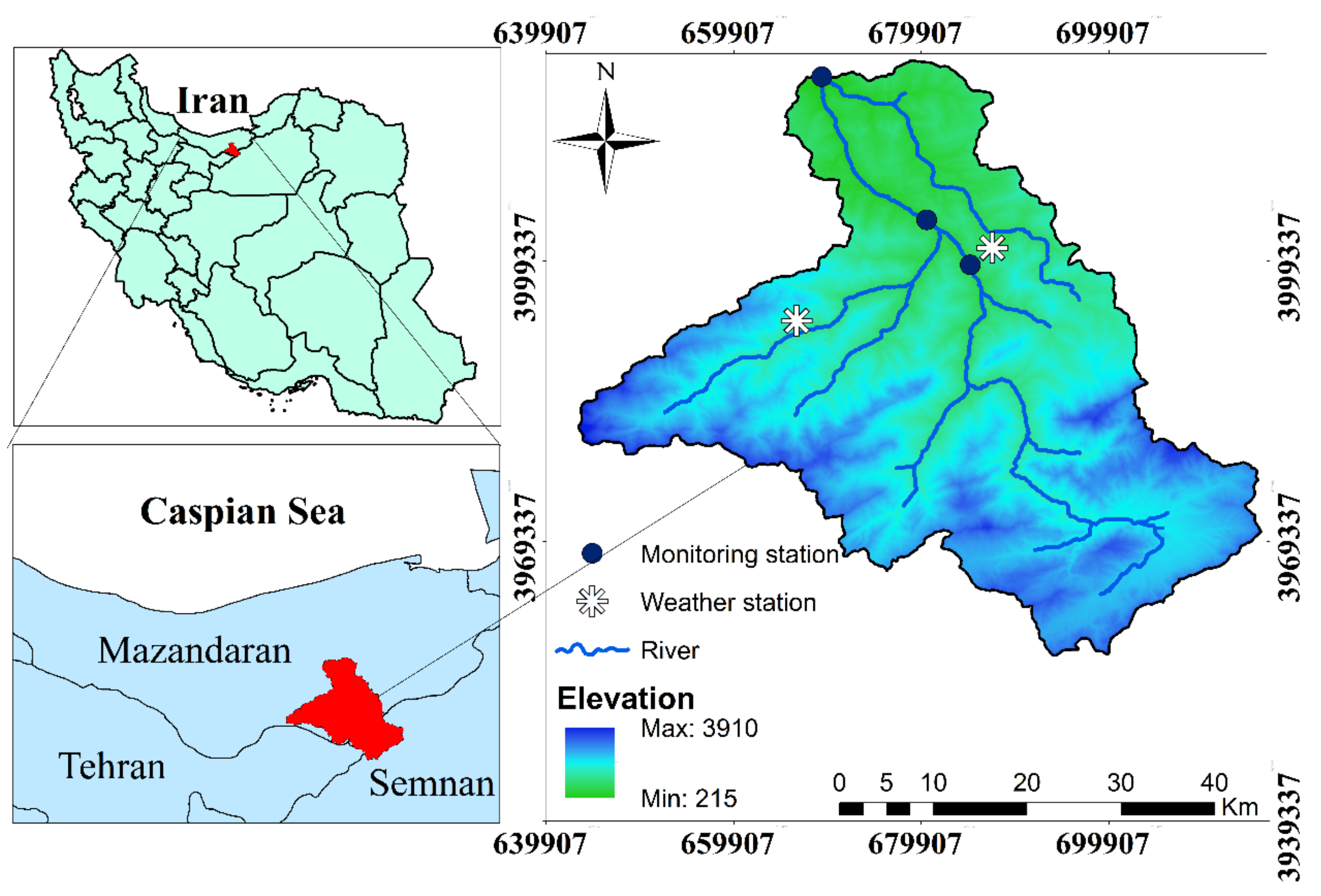
Talar River is a mountainous watershed with a total area of 210,088.7 ha, which is located between the eastern longitudes 52°35′22.2″ and 53°23′34.19″ and the northern latitudes 35°44′23.6″ and 36°19′1.6″ in Mazandaran province (Northern Iran). The average height is 2001.1 m a.s.l., and this region is characterized by a Mediterranean rainfall regime. The region has a mean annual rainfall of 552.7 mm and annual minimum and maximum temperature of 7.7 and 21.1 °C, respectively [44]. Figure 1 shows the location of Talar, which is also characterized by gentle steep hillslopes (less than 12%) and is mainly distributed between the southeast highland plains and land near the outlet of the watershed. The sloping areas (more than 60%) occupy 14.2% of the whole territory. The remaining 38% have inclinations greater than 30%. The lithology and stratigraphy of Talar watershed are diverse. Most of the area is covered by sedimentary, igneous and continental rocks [44]. Most of the rock units (about 61%) are related to the Mesozoic Era. Moreover, 58 types of soils with different physical and chemical properties have been registered. The average discharge for Shirgah station located at 52°53′10″ eastern longitude and 36°57′10″ northern latitude, registered 7.95 m3/s and the highest discharge was 93.46 m3/s (1971–1998). The most important land uses of the studied area are forests, dry land farming, irrigated lands, rangelands and residential areas [44].
2.2. SWAT Model
The SWAT model is a distributed, physics-based and continuous model that is used to perform simulations at the catchment scale. This model was developed to predict the impact of land use and land management practices on water, sediment and pollutant yields in large watersheds using a daily time step [28]. In the SWAT model, the main watershed is divided into multiple sub-watersheds, based on soil types, land uses and slope classes, resulting in hydrological response units (HRU). Soil water content, surface runoff, nutrient cycles, sediment yield, crop growth and management practices can be also simulated in each HRU [45].
The simulation of the hydrological cycle allows separation into a land phase and a water phase. The simulation of the land phase is based on water balance equations. The generated runoff in each HRU is summed to calculate the water reaching the main channel in each sub-basin. The water phase of the hydrological cycle is defined as the process of routing runoff in a river channel using the variable storage coefficient method. A detailed description of the model can be also found in Neitsch et al. [46].
SWAT is also able to simulate evapotranspiration, infiltration, percolation, runoff generation, nutrient cycling and transport for each HRU. Water and sediment routing as well as in-stream nutrient processes can be simulated along the channel length for each sub-basin [46]. The algorithms for nitrogen cycling and transport are based on the EPIC (Erosion-Productivity Impact Calculator) model [45]. Net mineralization is simulated with one active and one stable organic nitrogen pool. Plant uptake of nitrogen is estimated using a supply and demand approach. Finally, nitrates in soils can be removed from the soil via denitrification, mass flow of water as well as plant uptake [46].
2.3. Data Collection
In this study, SWAT version 2012 was used to simulate water quality and quantity affected by land use changes. The input data for the SWAT model for this study were weather data, a digital elevation model (DEM), soil and land-use, streamflow, and water quality data. A detailed description of these input data and their sources are presented in Table 1.
The land use data were generated from Landsat satellite images (Landsat Thematic Mapper (TM) for 1991 and Landsat Enhanced Thematic Mapper Plus (ETM+) for 2006, which were downloaded from the USGS website (Figure 2). Both images correspond to June. Land-use maps were generated using a supervised classification based on the maximum likelihood algorithm. Then, the overall accuracy and kappa coefficient (κ) were used to assess the classification accuracy. Land use data were classified into five different land use types including forest, irrigated land, dry land farming, rangeland and urban areas. To achieve these goals, the software ENVI Version 5.1 (Boulder, CO, USA) was used. In this study, for determining the land use scenario for 2050, parameters such as elevation classes, slope, distance from the river and roads as well as residential areas were used as indicators of land use change. After the image classification was completed for 1991 and 2006, the differences among land use classes were calculated between the two paired-periods. Then, by dividing this difference over a period of 15 years (1991–2006), the annual rate of change was obtained for each year. Finally, the land use polygons in the GIS environment were reduced by considering parameters.
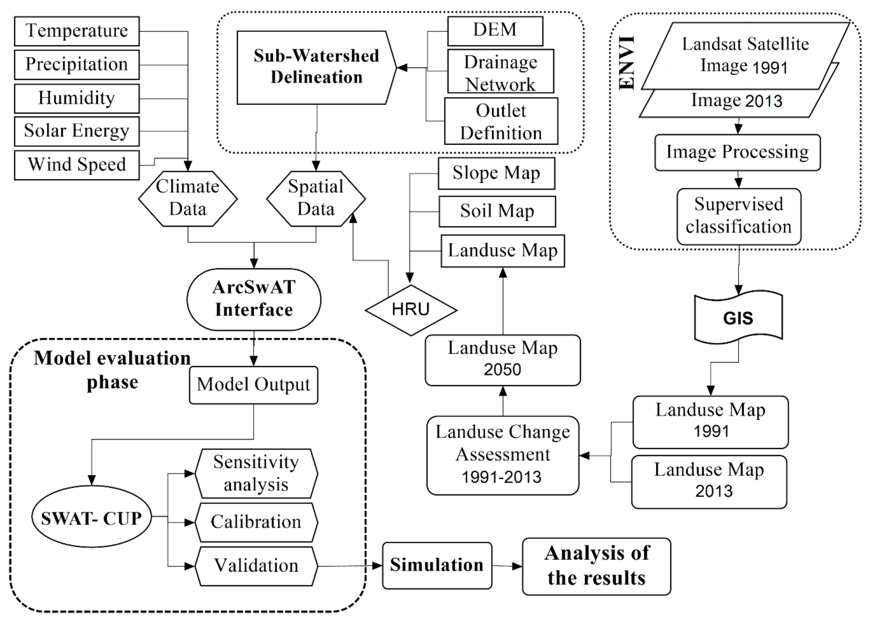
The watershed was delineated into 23 sub-watersheds using a digital elevation model. Then, the area based on special conditions of soil types, land uses and topography was divided into HRU units. Daily weather data (precipitation, maximum and minimum temperature, relative humidity, and wind speed and sunshine hours) were obtained from three local weather gauges from 1 January 2000 to 30 September 2013. The basic calibration and validation of SWAT were conducted using the land use map of 2013. Stream flow records were also measured daily using the hydrometric stations of Shirgah, Kerikola and Polsefid. The discharge data used were: (i) from 2001 to 2008 (for calibration) and (ii) 2009 to 2013 (for validation). Measurements of nitrate started in 2012 at the Shirgah station. We used 2012 and 2013 monthly nitrate data for calibration and validation, respectively. Figure 3 shows the stages of this research.
2.4. Model Performance Evaluation
Due to limitations related to the input data such as slope, elevation, soil type, land cover and complexity of hydrologic processes, the calibration of SWAT output was considered as complex. There are many statistical methods to access and evaluate the accuracy of model results. In this study, the accuracy of SWAT simulation was evaluated with the observed values using the coefficient of correlation (R2), Nash-Sutcliffe coefficient (ENS) and percent bias (PBIAS).
2.4.1. Coefficient of Determination (R2)
This method is considered a good indicator to determine the data uniformity observed and simulated. R2 ranges from 0 to 1, where higher values indicate less error variance [47] and values greater than 0.50 are considered acceptable [48]. R2 was calculated using Equation (1):
where observed stream flow in m3/s; = simulated stream flow in m3/s; mean of n values; Mean of simulated values and mean of observed values and n = number of observations.
2.4.2. Nash-Sutcliffe Efficiency (NSE)
NSE is a normalized statistical method that assesses the relative magnitude of the residual variance compared to measured data variance [49]. NSE was calculated using Equation (2):
NSE ranges between −∞ and 1.0; a value of 1 is the optimal value. Values between 0.0 and 1.0 are generally viewed as acceptable levels of performance. Generally, the model simulation was considered satisfactory if NES > 0.5 [47].
2.4.3. Percent Bias (PBIAS)
PBIAS allows calculation of the average tendency of the simulated values to be larger or smaller than their observed values [50]. A model with low-magnitude values from PBIAS indicates accurate simulation (optimal value is 0). Positive and negative values of PBIAS indicated that the model registered an underestimation or overestimation bias, respectively [50]. PBIAS was obtained as follows from Equation (3):
where PBIAS is the deviation of data being evaluated, expressed as a percentage. Table 2 shows the classification of statistical results of NSE and PBIAS for flow and nutrients [47].
2.4.4. Sensitivity Analysis
In this study, Swat Cup software and the SUFI-2 program were used to conduct the sensitivity analysis, calibration and validation. Many parameters are able to affect the model results; therefore, it is necessary to specify the key parameters that will register more impact. In our case, 24 parameters were selected using monthly observational discharge (2001–2003) and nitrate (2012–2013) data. Sensitivity analysis was automatically performed with 500 iterations and 24 sensitivity parameters.
3. Results and Discussion
3.1. Accuracy Assessment of Land Use Classification
It is well known that the accuracy assessment is the most important part of remote sensing classification and land use change classifications. Lu et al. [51] stated that the most common accuracy assessment elements include overall accuracy, producer’s accuracy, user’s accuracy and the Kappa coefficient. In this study, the Kappa coefficient and overall accuracy were also used to assess the verification of land use classification (Table 3 and Table 4).
Forest, irrigated land, dry land farming and residential areas in 1991 were accurately classified using the error matrix (Table 3). Residential areas and irrigated land are sometimes mistaken for range land. This may be due to the proximity of these land uses to rangeland areas. The classification error matrix in 2006 shows that dry land farming was accurately classified, followed by forest, residential areas, irrigated land and range lands (Table 4). In 1991 and 2013, the classification efficiency reached 96.7% and 87.2%, respectively, and the corresponding kappa coefficient was 0.94 and 0.80.
3.2. Land Use Changes from 1991 to 2013
A total of five land use classes were identified from the satellite images, including forest, irrigated land, dry land farming, range land and residential areas.
In Table 5, land use changes are summarized. Land use maps obtained using Landsat TM and ETM images of Talar River for 1999 and 2013 are displayed in Figure 4.
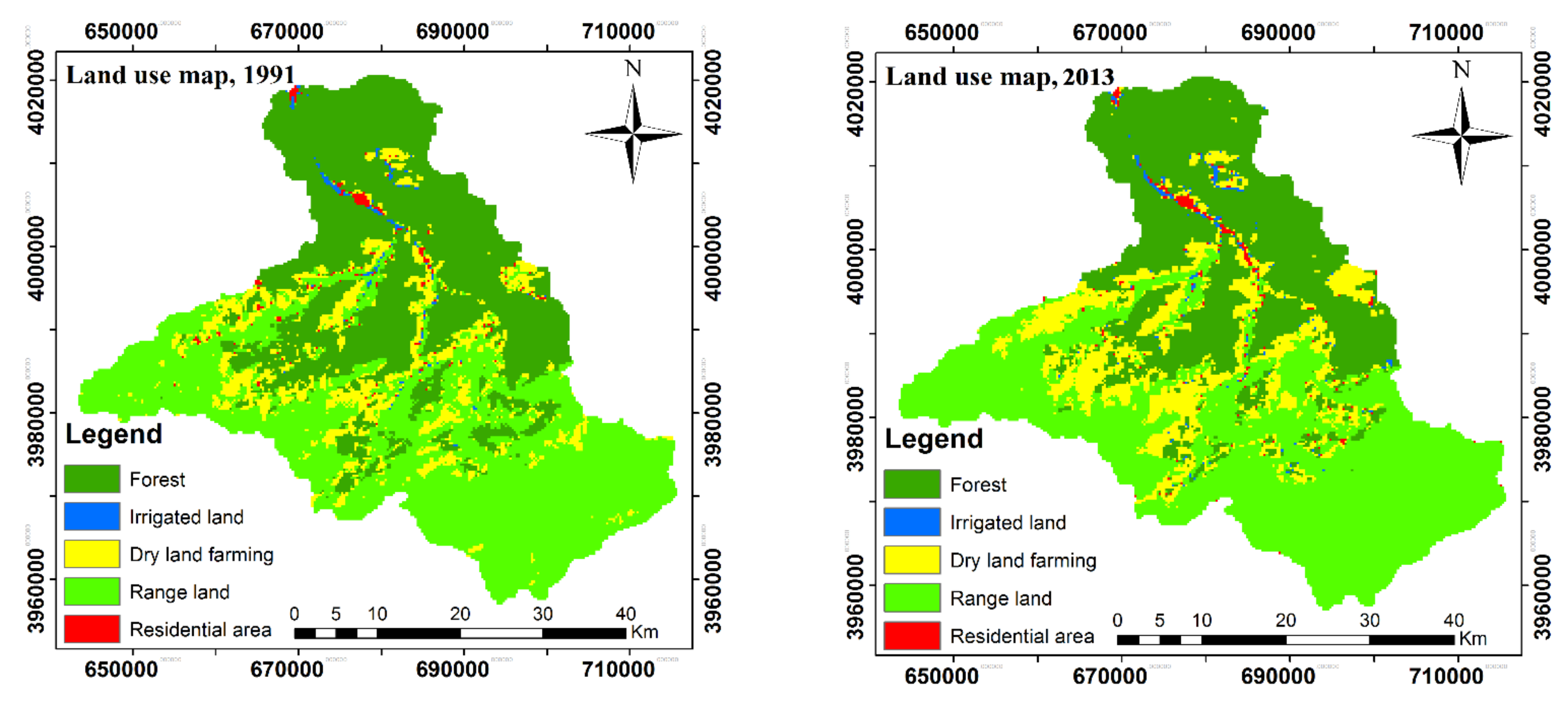
It can be observed that the dominant land uses are forest and range lands with total areas of about 80% (Table 5). The 1991 land use map shows that the forest, irrigated land, dry land farming, range land and residential areas had respective areas of 40.8%, 0.5%, 11.3%, 46.6% and 0.8% (Figure 3a), but the land use map shows that forest, irrigated land, dry land farming, range land and residential areas had areas of 34.8%, 0.7%, 14.8%, 48.8% and 0.9% in 2013 (Figure 3b). From 1991 to 2013, forest decreased from 40.8 to 34.8% but other land uses increased (Table 5 and Figure 3). This dynamic has been reported in several areas around the world such as in the Mediterranean landscapes or tropical territories, showing critical land degradation processes such as soil erosion or a decrease in soil fertility after these changes [52,53,54]. Therefore, land planners and policy makers should detect these drastic land use changes and apply restoration measures or strict plans to protect forestry areas and rural areas that use water for traditional agricultural activities [55,56].
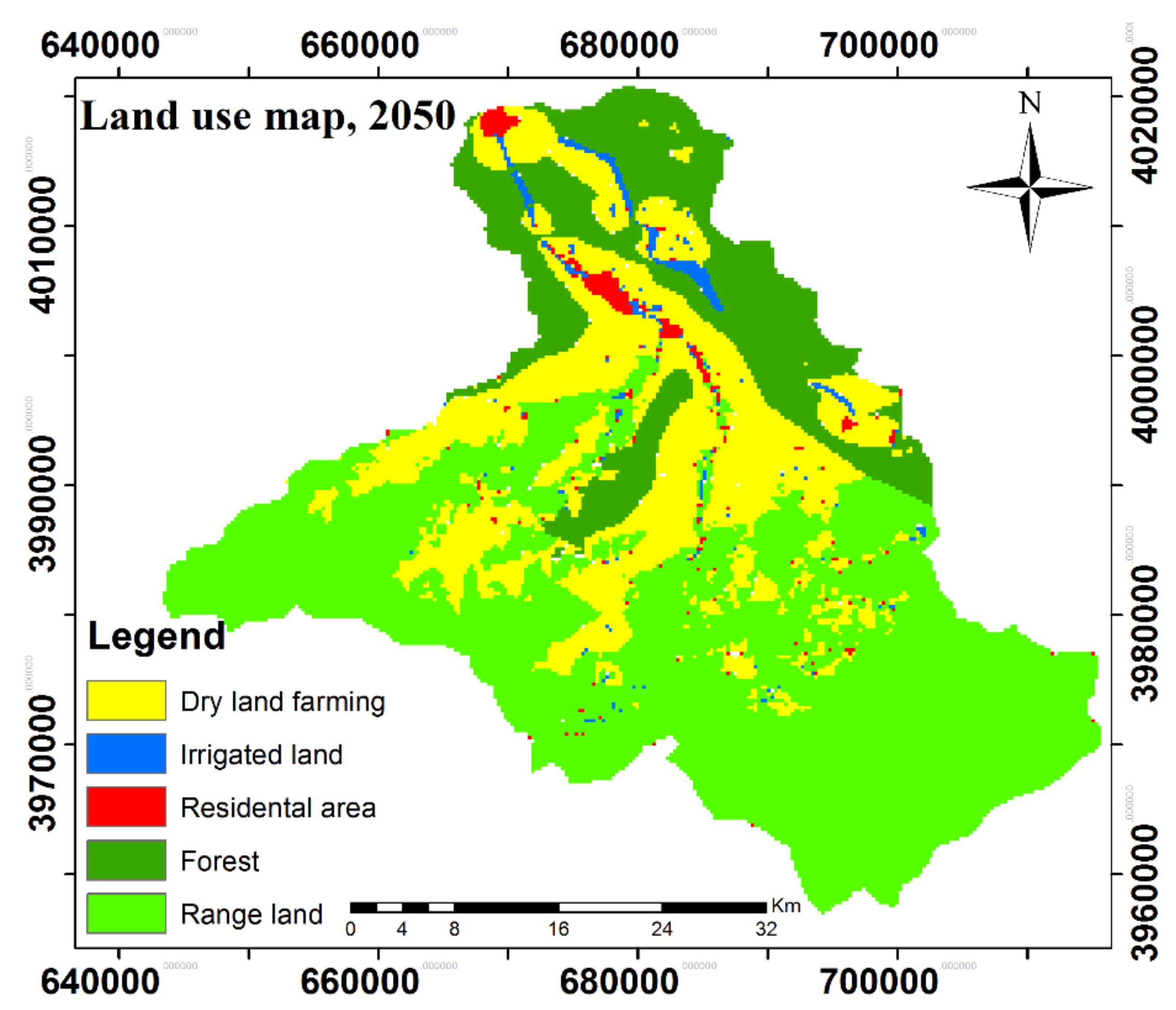
3.3. Land-Use Scenario in Year 2050
During the last twenty years, a loss of forestry areas has been registered. Thus, we try to evaluate the impact of land use changes on water flow and nitrate transport for a future scenario. To achieve this goal, three land use scenarios are chosen: 1991 (S1), 2013 (S2) and 2050 (S3). The image classification is presented in Table 6. Figure 5 shows land-use scenarios for the year 2050. As other authors observed, parameters such as slope, distance from roads and residential areas affected land use polygon size [57]. We can observe that the outlook for future water quality of rainwater harvesting systems is not so hopeful. Our results show that a decrease in natural areas and an increase in human expansion would be higher than nowadays. It is important to remark that several authors claimed that the loss of forestry areas is affecting the levels of carbon, ozone and biodiversity [58,59]. Moreover, the risk of floods and slides may also increase, as demonstrated other authors in other Iranian areas [60,61,62].
3.4. Model Calibration and Validation
3.4.1. Sensitivity Analysis
Because of different characteristics of watersheds such as soil physical and chemical properties, land use and physiographic characteristics, the effects of parameters can vary with respect to hydrology, sediment and nutrient discharges [63,64]. Hence, parameter sensitivity analysis must locally performed although none of the sensitivity analysis methods is clearly superior [65].
Since water quality models have comprehensive parameters and there are various data to compare with simulation results (e.g., flow, suspended sediment, nitrogen and phosphorus), sensitivity analysis methods are needed in order to adjust parameters considering the model outputs [66]. In this study, the selected parameters for sensitivity analysis based on relevant literature [67] and SWAT documentation [27,46] are presented in Table 7. The soil conservation service curve number (SCS-CN) was considered in this study as the most sensitive parameter for the three stations and the main parameter for flow simulation.
The other most sensitive parameters are SMTMP, SOL_BD, ALPHA_BNK, SOL_K, SOL_AWC, SMFMN, SLSUBBSN and REVAPMN. The last-ranked flow parameters are LAT_TTIME, CANMX, TIMP, CH_N2, GWQMN, SURLAG, TLAPS, ESCO, GW_REVAP and ALPHA_BF, (meaning in Table 7). Also, for nitrogen discharge, the most sensitive parameters are CN2, and GWQMN and ALPHA_BF and also water quality parameters SDNCO, ERORGN, SOL_NO3 and SOL_ORGN (meaning in Table 7).
Lenhart et al. [68] and Zhai et al. [69] reported that CN2 (SCS runoff curve number for moisture condition II) was also the most sensitive parameters in the simulation of flow and water quality. They explained that this is because the land use and soil types often have a great influence on the CN2 value [70]. As a consequence, this parameter has a major influence on the composition of the water balance and the simulated flow [71].
3.4.2. Stream Flow Simulations
The model simulation was evaluated for both the calibration and validation periods using graphical comparisons and three statistical measures (Table 8): R2, NSE and PBIAS.
Prior to model calibration, the mean of the simulated stream flow data for Shirgah, Kerikkola and Polsefid relative to the mean observed data was approximately 1.4, 2.6 and 0.02%, respectively. For calibration (2001–2008) and validation (2009–2013) periods, NSE and R2 ranged from 0.57 to 0.75 and 0.62 to 0.76, respectively, for the three monitored stations. The monthly flow simulations show a good calibration and validation based on the performance ratings of Moriasi et al. [47] with rates of 0.65 < NSE < 0.75 and ±10 < PBIAS < ±15. The PBIAS coefficient for calibration and validation period ranges from 1.3% to 13%. These results show an underestimation of the simulated mean.
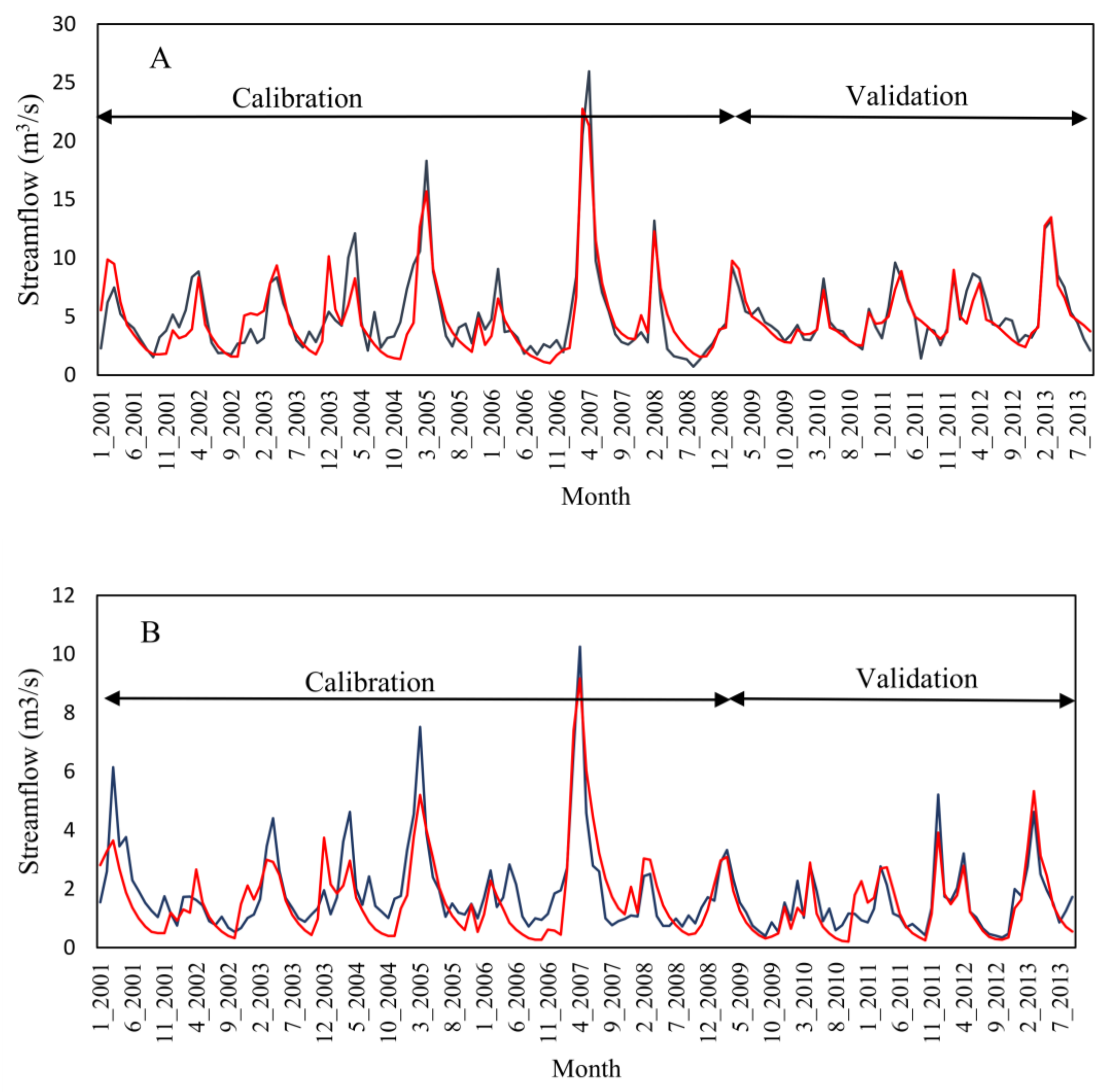
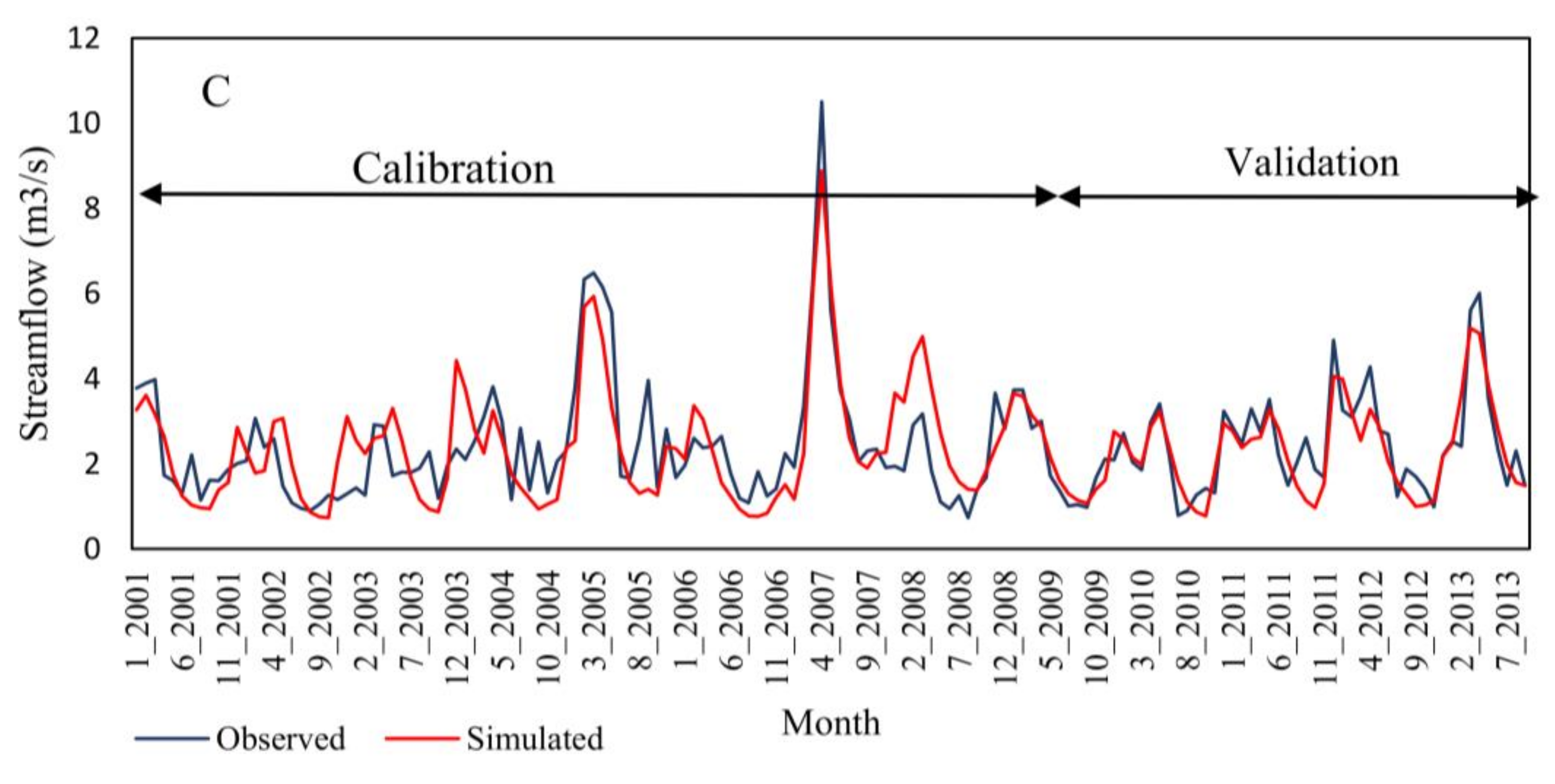
In Figure 6, hydrographs of observed and simulated monthly flow at Shirgah, Kerikkola and Polseffid stations during 2001–2008 (calibration period) and 2009–2013 (validation period) are presented. We can appreciate that time and the volume of flow peaks are simulated with high accuracy, but the maximum flow volume of most peaks is underestimated. In general, the model statistical evaluations indicate a good model performance for flow simulation in Talar watershed. Our findings agree with those presented by Cao et al. [72], who, using SWAT, also noted that the number and location of rainfall gauges strongly affected the accuracy of the flow simulation. Wu and Chen [73] also detected similar results, but they had better coefficients in their studies. They obtained an NSE and R2 of 0.75 and 0.80 for the calibration period, and 0.74 and 0.87 for the validation period using SWAT-cup and SUFI-2, respectively. Moreover, they were able to report reasonable consistency among the simulated and observed runoff values as well as the responses to the precipitation dynamic. In another case, Xu et al. [74] compared climate data measured at Xingshan climate station and gridded climate data for the accuracy of the simulation result. They stated that the gridded dataset had lower accuracy of stream flow predictions, and for this reason, gridded climate data were not used for improving simulation results.
3.4.3. Nitrate Simulations
The concentration of nitrates in water is also considered an important indicator to evaluate the water quality of rainwater harvesting systems. Figure 7 shows the monthly measured and simulated nitrate loads for calibration and validation periods (2012 and 2013).
The model has calibration and validation values close to the measured values for most of the monthly nitrate loads (Figure 7). These results are also confirmed by our statistical measures in Table 8. The model efficiency NSE for calibration and validation periods is 0.74 and 0.62, respectively, and the R2 coefficient for calibration and validation periods is 0.75 and 0.83, respectively. PBIAS is 5.4 (for calibration period) and −39.3 (for validation period). These results show that the model has a general underestimation (in first period) and a high overestimation (in second period). Similarly, the model performance in simulating nitrate loads for both calibration and validation periods can be considered suitable (with 0.65 > NSE > 0.75, ±10 < PBIAS < ±40) [46] and acceptable in stream flow and nitrate simulations. In this study, the result of nitrate simulation is close to that for other catchments like the Lam Takong River Basin in Thailand [75]. These authors obtained R2 values higher than 0.6 and PBIAS values lower than 25% for nitrate simulation. Moreover, they established fair relationships between observation and simulation results.
3.5. Discharge and Nitrate Responses to Land Use Changes
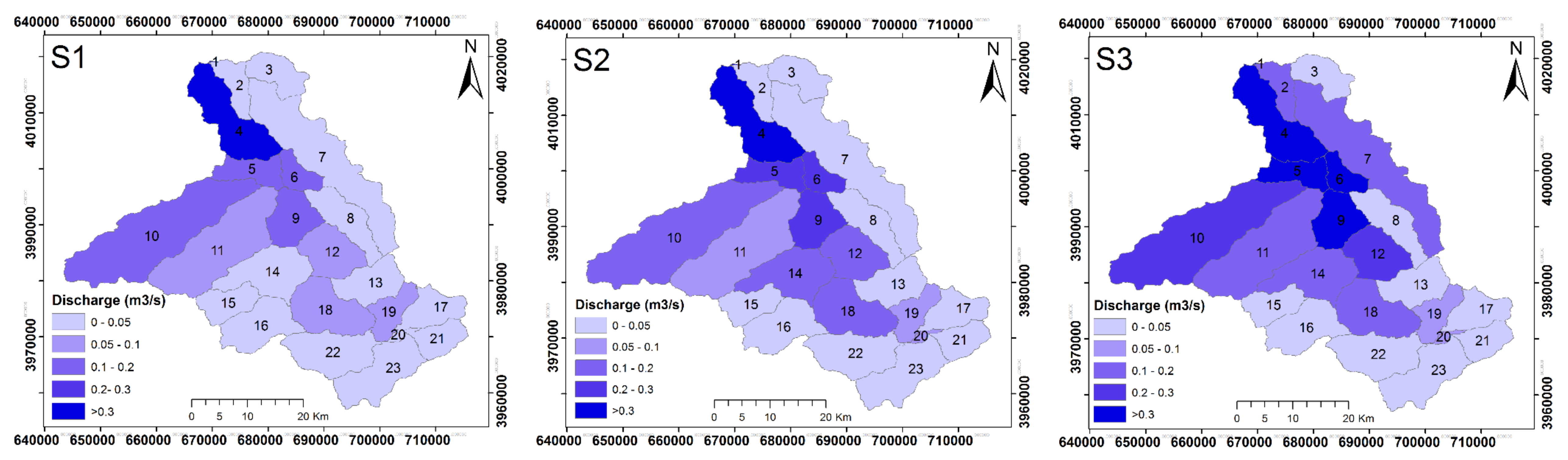
Table 9 shows the percentile changes of discharge and nitrate at the sub-basin scale under three land use change scenarios. For both the first period (1991–2013) and the second period (2013–2050), the discharge increases in most sub-basins because of deforestation and the development of rainfed and irrigated agricultural land. The water discharges do not change in some sub-basins such as 3, 8 and 21 (in the first period) and sub-basins 3 and 13 (in the second period). Additionally, the highest changes in discharge are registered in sub-basins 22, 7 and 2, (in three periods). Nitrate output shows an increase, except in sub-basin 3 and 8 for the S1-S2 scenario. The highest nitrate output observed in the sub-basin is located in sub-basin 13, with a rate of 613.4% (Table 9). In addition, nitrate output increases for almost all sub-basins for the S2-S3 scenario. Here, the highest nitrate rate is calculated for sub-basins 23, 15 and 16, with rates of 1277.6, 1240.54 and 3820.7, respectively. The third scenario (S1-S3) shows a sharp increase in nitrate output in several sub-basins, except 8 and 16.
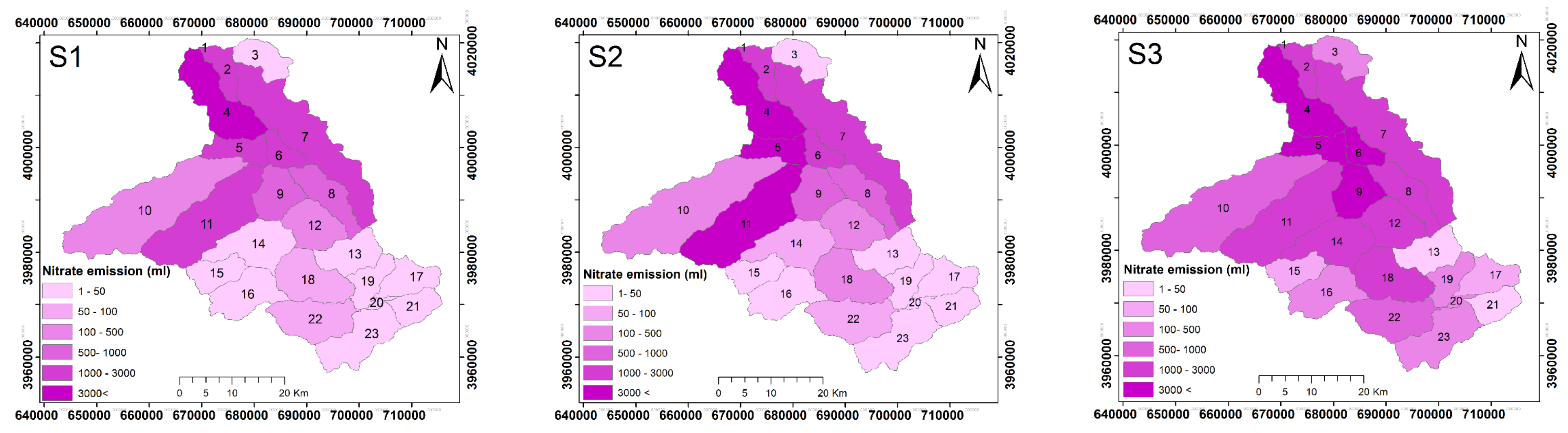
Figure 8 and Figure 9 show the changes in average annual discharge and nitrate yield in all sub-basins for the three land use scenarios. The results also show that forest destruction and the development of dry land farming are causing a higher concentration of nitrates in surface water. In general, the results state that the nitrate loss originates from agricultural lands and rangelands, which can be considered as driving factors of water quality [76]. We conclude that these areas are the main sources of nitrate pollution in Talar watershed, being located in the hotspot of dry land farming, which affects irrigated and forestry areas. The obtained results correspond with the conclusions of Ahearn et al. [77], Behera and Panda [78] and Mohammad and Ahmad [79], who claimed that dry land farming is one of the most important land uses that is able to affect nitrate mobilization. Castillo et al. [80] also reported that nitrate is significantly related to the water quality of rainwater harvesting systems and the elimination of forestry areas in the catchments. In fact, apart from other many factors, forest land and irrigated areas are identified as a sink for NPS pollution [81,82] because decayed organic matter from forest land can produce organic nutrients and cause nutrient loss during rainfall.
3.6. Broader Impact
In recent years, the Mazandaran province has experienced widespread land use changes due to its favorable climatic conditions and fertile soils, population growth and food demand needs. A large amount of forest land has been turned into garden and agriculture land uses. Due to a recent water shortage, a large amount of riverside land is devoted to rice cultivation due to easy access to water. These extensive land use changes in Mazandaran province endanger water and soil resources in watersheds and sustainable development. These results can be extrapolated to other areas with similar environmental problems applying the same methods and increasing the scales. Thus, we consider that this study can show a broader impact and be useful for land managers and decision makers in the future.
4. Conclusions
In this study, an evaluation of the impact of land use changes on water quality of runoff water harvesting systems of the Talar River watershed, using satellite data and the SWAT model, was conducted. We conclude that the combination of both techniques is able to provide useful information to analyze spatiotemporal land use dynamics and water quality of rainwater harvesting systems. The simulated flow and nitrate loads were in reasonable agreement with the measured values using statistical coefficients such as R2, NSE and PBIAS. The results of land use scenarios for all sub-basins indicated that the flow and nitrate increased, with rates of 34.4% and 42.2% in the first period (1991–2013) and 42.3%, and 55.9% in the second period (2013–2050), respectively. The spatial modeling and assessment of water and nitrate yield presented may allow better understanding of the land use change challenges in Talar River watershed. Moreover, the results will allow researchers, managers and policy makers to identify critical areas, appropriate land use management plans and pollution control measures.
Acknowledgments
We appreciate the Sari Agricultural Sciences and Natural Resources University (SANRU) for financial support.
Author Contributions
Ataollah Kavian, Maziar Mohammadi, Leila Gholami conceived and designed the experiments, performed the experiments, analyzed the data and contributed reagents/materials/analysis tools. Ataollah Kavian and Jesús Rodrigo-Comino wrote the paper.
Conflicts of Interest
The authors declare no conflict of interest. The founding sponsors had no role in the design of the study; in the collection, analyses, or interpretation of data; in the writing of the manuscript, and in the decision to publish the results.
References
- Keesstra, S.D. Impact of natural reforestation on floodplain sedimentation in the Dragonja basin, SW Slovenia. Earth Surf. Process. Landf. 2007, 32, 49–65. [Google Scholar] [CrossRef]
- Mohajerani, H.; Kholghi, M.; Mosaedi, A.; Farmani, R.; Sadoddin, A.; Casper, M. Application of bayesian decision networks for groundwater resources management under the conditions of high uncertainty and data scarcity. Water Resour. Manag. 2017, 31, 1859–1879. [Google Scholar] [CrossRef]
- Bertalan, L.; Tóth, C.A.; Szabó, G.; Nagy, G.; Kuda, F.; Szabó, S. Confirmation of a theory: Reconstruction of an alluvial plain development in a flume experiment. Erdkunde 2016, 70, 271–285. [Google Scholar] [CrossRef]
- Abdollahi, Z.; Kavian, A.; Sadeghi, S.H.R. Spatio-temporal changes of water quality variables in a highly disturbed river. Glob. J. Environ. Sci. Manag. 2017, 3, 243–256. [Google Scholar] [CrossRef]
- Steffan, J.J.; Brevik, E.C.; Burgess, L.; Cerdà, A. The effect of soil on human health: An overview. Eur. J. Soil Sci. 2017, 69, 159–171, In press. [Google Scholar] [CrossRef] [PubMed]
- Jafarian, Z.; Kavian, A. Effects of Land-Use Change on Soil Organic Carbon and Nitrogen. Commun. Soil Sci. Plant Anal. 2013, 44, 339–346. [Google Scholar] [CrossRef]
- Pulido Moncada, M.; Gabriels, D.; Cornelis, W.; Lobo, D. Comparing Aggregate Stability Tests for Soil Physical Quality Indicators. Land Degrad. Dev. 2015, 26, 843–852. [Google Scholar] [CrossRef]
- Khaledian, Y.; Kiani, F.; Ebrahimi, S.; Brevik, E.C.; Aitkenhead-Peterson, J. Assessment and monitoring of soil degradation during land use change using multivariate analysis. Land Degrad. Dev. 2016, 28, 128–141. [Google Scholar] [CrossRef]
- Schultz, B. Impacts of man-Induced Changes in Land use and Climate Change on Living in Coastal and Deltaic Areas. Irrig. Drain. 2016. [Google Scholar] [CrossRef]
- Pulido, M.; Schnabel, S.; Lavado Contador, J.F.; Lozano-Parra, J.; González, F. The Impact of Heavy Grazing on Soil Quality and Pasture Production in Rangelands of SW Spain. Land Degrad. Dev. 2018, 29, 219–230. [Google Scholar] [CrossRef]
- Jacobson, C.R. Identification and quantification of the hydrological impacts of imperviousness in urban catchments: A review. J. Environ. Manag. 2011, 92, 1438–1448. [Google Scholar] [CrossRef] [PubMed]
- Martínez-Hernández, C.; Rodrigo-Comino, J.; Romero-Díaz, A. Impact of lithology and soil properties on abandoned dryland terraces during the early stages of soil erosion by water in south-east Spain. Hydrol. Process. 2017, 31, 3095–3109. [Google Scholar] [CrossRef]
- Pfister, L.; Kwadijk, J.; Musy, A.; Bronstert, A.; Hoffmann, L. Climate change, land use change and runoff prediction in the Rhine–Meuse basins. River Res. Appl. 2004, 20, 229–241. [Google Scholar] [CrossRef]
- Kavian, A.; Golshan, M.; Abdollahi, Z. Flow discharge simulation based on land use change predictions. Environ. Earth Sci. 2017, 76, 588. [Google Scholar] [CrossRef]
- Wang, W.; Shao, Q.; Yang, T.; Peng, S.; Xing, W.; Sun, F.; Luo, Y. Quantitative assessment of the impact of climate variability and human activities on runoff changes: A case study in four catchments of the Haihe River basin, China. Hydrol. Process. 2012, 27, 1158–1174. [Google Scholar] [CrossRef]
- Angrill, S.; Petit-Boix, A.; Morales-Pinzón, T.; Josa, A.; Rieradevall, J.; Gabarrell, X. Urban rainwater runoff quantity and quality—A potential endogenous resource in cities? J. Environ. Manag. 2017, 189, 14–21. [Google Scholar] [CrossRef] [PubMed]
- Shamir, E.; Rimmer, A.; Georgakakos, K.P. The use of an orographic precipitation model to assess the precipitation spatial distribution in Lake Kinneret watershed. Water 2016, 8, 591. [Google Scholar] [CrossRef]
- Germer, S.; Neill, C.; Vetter, T.; Chaves, J.; Krusche, A.V.; Elsenbeer, H. Implications of long-term land-use change for the hydrology and solute budgets of small catchments in Amazonia. J. Hydrol. 2009, 364, 349–363. [Google Scholar] [CrossRef]
- Giertz, S.; Junge, B.; Diekkrüger, B. Assessing the effects of land use change on soil physical properties and hydrological processes in the sub-humid tropical environment of West Africa. Phys. Chem. Earth Parts A/B/C 2005, 30, 485–496. [Google Scholar] [CrossRef]
- Zema, D.A.; Denisi, P.; Taguas Ruiz, E.V.; Gómez, J.A.; Bombino, G.; Fortugno, D. Evaluation of Surface Runoff Prediction by AnnAGNPS Model in a Large Mediterranean Watershed Covered by Olive Groves. Land Degrad. Dev. 2015, 27, 811–822. [Google Scholar] [CrossRef]
- Rodrigo-Comino, J.; Cerdà, A. Improving stock unearthing method to measure soil erosion rates in vineyards. Ecol. Indic. 2018, 85, 509–517. [Google Scholar] [CrossRef]
- Lin, B.; Chen, X.; Yao, H.; Chen, Y.; Liu, M.; Gao, L.; James, A. Analyses of landuse change impacts on catchment runoff using different time indicators based on SWAT model. Ecol. Indic. 2015, 58, 55–63. [Google Scholar] [CrossRef]
- Beasley, D.B.; Huggins, L.F.; Monke, E.J. ANSWERS: A Model for Watershed Planning. Trans. ASAE 1980, 23, 938–944. [Google Scholar] [CrossRef]
- Young, R.A.; Onstad, C.A.; Bosch, D.D.; Anderson, W.P. AGNPS: A nonpoint-source pollution model for evaluating agricultural watersheds. J. Soil Water Conserv. 1989, 44, 168–173. [Google Scholar]
- Bicknell, B.; Imhoff, J.; Kittle, J.; Donigian, A.; Johanson, R. Hydrologic Simulation Program-Fortran: User’s Manual for Release 10; U.S. EPA Environmental Research Laboratory Athens: Athens, GA, USA, 1993.
- Nearing, M.A.; Foster, G.R.; Lane, L.J.; Finkner, S.C. A Process-Based Soil Erosion Model for USDA-Water Erosion Prediction Project Technology. Trans. ASAE 1989, 32, 1587–1593. [Google Scholar] [CrossRef]
- Williams, J.R.; Nicks, A.D.; Arnold, J.G. Simulator for Water Resources in Rural Basins. J. Hydraul. Eng. 1985, 111, 970–986. [Google Scholar] [CrossRef]
- Arnold, J.G.; Srinivasan, R.; Muttiah, R.S.; Williams, J.R. Large area hydrologic modeling and assessment part i: Model development1. JAWRA J. Am. Water Resour. Assoc. 2007, 34, 73–89. [Google Scholar] [CrossRef]
- Zhang, P.; Liu, Y.; Pan, Y.; Yu, Z. Land use pattern optimization based on CLUE-S and SWAT models for agricultural non-point source pollution control. Math. Comput. Model. 2013, 58, 588–595. [Google Scholar] [CrossRef]
- Tong, S.T.Y.; Liu, A.J.; Goodrich, J.A. Assessing the water quality impacts of future land-use changes in an urbanising watershed. Civ. Eng. Environ. Syst. 2009, 26, 3–18. [Google Scholar] [CrossRef]
- Chaplot, V.; Saleh, A.; Jaynes, D.B.; Arnold, J. Predicting Water, Sediment and NO3-N Loads under Scenarios of Land-use and Management Practices in a Flat Watershed. Water Air Soil Pollut. 2004, 154, 271–293. [Google Scholar] [CrossRef]
- Kigira, F.K.; Gathenya, J.M.; Home, P.G. Modeling the Influence of Land Use/Land Cover Changes on Sediment Yield and Hydrology in Thika River Catchment Kenya, Using SWAT Model. In Proceedings of the 2007 JKUAT Scientific, Technological and Industrialisation Conference, JKUAT, Kenya, 25–26 October 2007. [Google Scholar]
- Lam, Q.D.; Schmalz, B.; Fohrer, N. The impact of agricultural Best Management Practices on water quality in a North German lowland catchment. Environ. Monit. Assess. 2011, 183, 351–379. [Google Scholar] [CrossRef] [PubMed]
- Ouyang, W.; Song, K.; Wang, X.; Hao, F. Non-point source pollution dynamics under long-term agricultural development and relationship with landscape dynamics. Ecol. Indic. 2014, 45, 579–589. [Google Scholar] [CrossRef]
- Li, Y.; Chang, J.; Wang, Y.; Jin, W.; Guo, A. Spatiotemporal Impacts of Climate, Land Cover Change and Direct Human Activities on Runoff Variations in the Wei River Basin, China. Water 2016, 8, 220. [Google Scholar] [CrossRef]
- Giri, S.; Nejadhashemi, A.P.; Woznicki, S.; Zhang, Z. Analysis of best management practice effectiveness and spatiotemporal variability based on different targeting strategies. Hydrol. Process. 2012, 28, 431–445. [Google Scholar] [CrossRef]
- Stehr, A.; Debels, P.; Romero, F.; Alcayaga, H. Hydrological modelling with SWAT under conditions of limited data availability: Evaluation of results from a Chilean case study. Hydrol. Sci. J. 2008, 53, 588–601. [Google Scholar] [CrossRef]
- Keshavarzi, A.; Tuffour, H.; Bagherzadeh, A.; Duraisamy, V. Spatial and Fractal Characterization of Soil Properties across Soil Depth in an Agricultural Field, Northeast Iran. Eur. J. Soil Sci. 2018, 7, 35–45. [Google Scholar]
- Zeraatpisheh, M.; Ayoubi, S.; Jafari, A.; Finke, P. Comparing the efficiency of digital and conventional soil mapping to predict soil types in a semi-arid region in Iran. Geomorphology 2017, 285, 186–204. [Google Scholar] [CrossRef]
- Kavian, A.; Sabet, S.H.; Solaimani, K.; Jafari, B. Simulating the effects of land use changes on soil erosion using RUSLE model. Geocarto Int. 2017, 32, 97–111. [Google Scholar] [CrossRef]
- Luo, P.; He, B.; Chaffe, P.L.B.; Nover, D.; Takara, K.; Rozainy, M.A.Z.M.R. Statistical analysis and estimation of annual suspended sediments of major rivers in Japan. Environ. Sci. Process. Impacts 2013, 15, 1052–1061. [Google Scholar] [CrossRef] [PubMed]
- Luo, P.; He, B.; Takara, K.; Xiong, Y.E.; Nover, D.; Duan, W.; Fukushi, K. Historical assessment of Chinese and Japanese flood management policies and implications for managing future floods. Environ. Sci. Policy 2015, 48, 265–277. [Google Scholar] [CrossRef]
- Luo, P.; He, B.; Duan, W.; Takara, K.; Nover, D. Impact assessment of rainfall scenarios and land-use change on hydrologic response using synthetic Area IDF curves. J. Flood Risk Manag. 2015, 11, S84–S97. [Google Scholar] [CrossRef]
- Comprehensive studies of Talar watershed. Office of Watersheds Studies Evaluation; Jahad Engineering Services Company: Sari, Mazandaran, Iran, 2001. [Google Scholar]
- Jimmy, R. Williams Flood Routing With Variable Travel Time or Variable Storage Coefficients. Trans. ASAE 1969, 12, 100–103. [Google Scholar] [CrossRef]
- Neitsch, S.; Arnold, J.; Kiniry, J.; Williams, J. Soil and Water Assessment Tool Theoretical Documentation; Version 2000; Texas Water Resources Institute: College Station, TX, USA, 2009. [Google Scholar]
- Moriasi, D.N.; Arnold, J.G.; Van Liew, M.W.; Bingner, R.L.; Harmel, R.D.; Veith, T.L. Model Evaluation Guidelines for Systematic Quantification of Accuracy in Watershed Simulations. Trans. ASABE 2007, 50, 885–900. [Google Scholar] [CrossRef]
- Santhi, C.; Arnold, J.G.; Williams, J.R.; Dugas, W.A.; Srinivasan, R.; Hauck, L.M. Validation of the swat model on a large rwer basin with point and nonpoint sources. J. Am. Water Resour. Assoc. 2007, 37, 1169–1188. [Google Scholar] [CrossRef]
- Nash, J.E.; Sutcliffe, J.V. River flow forecasting through conceptual models part I—A discussion of principles. J. Hydrol. 1970, 10, 282–290. [Google Scholar] [CrossRef]
- Gupta, H.V.; Sorooshian, S.; Yapo, P.O. Status of Automatic Calibration for Hydrologic Models: Comparison with Multilevel Expert Calibration. J. Hydrol. Eng. 1999, 4, 135–143. [Google Scholar] [CrossRef]
- Lu, D.; Mausel, P.; Brondízio, E.; Moran, E. Change detection techniques. Int. J. Remote Sens. 2004, 25, 2365–2401. [Google Scholar] [CrossRef]
- Butzer, K.W. Environmental history in the Mediterranean world: Cross-disciplinary investigation of cause-and-effect for degradation and soil erosion. J. Archaeol. Sci. 2005, 32, 1773–1800. [Google Scholar] [CrossRef]
- García-Ruiz, J.M.; Nadal-Romero, E.; Lana-Renault, N.; Beguería, S. Erosion in Mediterranean landscapes: Changes and future challenges. Geomorphology 2013, 198, 20–36. [Google Scholar] [CrossRef] [Green Version]
- Panagos, P.; Meusburger, K.; Ballabio, C.; Borrelli, P.; Alewell, C. Soil erodibility in Europe: A high-resolution dataset based on LUCAS. Sci. Total Environ. 2014, 479–480, 189–200. [Google Scholar] [CrossRef] [PubMed] [Green Version]
- Benvenuti, S.; Bretzel, F. Agro-biodiversity restoration using wildflowers: What is the appropriate weed management for their long-term sustainability? Ecol. Eng. 2017, 102, 519–526. [Google Scholar] [CrossRef]
- Dawson, L.; Elbakidze, M.; Angelstam, P.; Gordon, J. Governance and management dynamics of landscape restoration at multiple scales: Learning from successful environmental managers in Sweden. J. Environ. Manag. 2017, 197, 24–40. [Google Scholar] [CrossRef] [PubMed]
- Ye, L.; Cai, Q.; Liu, R.; Cao, M. The influence of topography and land use on water quality of Xiangxi River in Three Gorges Reservoir region. Environ. Geol. 2009, 58, 937–942. [Google Scholar] [CrossRef]
- Barbier, E.B.; Delacote, P.; Wolfersberger, J. The economic analysis of the forest transition: A review. J. For. Econ. 2017, 27, 10–17. [Google Scholar] [CrossRef]
- Bravo-Espinosa, M.; Mendoza, M.E.; CarlóN Allende, T.; Medina, L.; Sáenz-Reyes, J.T.; Páez, R. Effects of converting forest to avocado orchards on topsoil properties in the trans-Mexican volcanic system, Mexico. Land Degrad. Dev. 2014, 25, 452–467. [Google Scholar] [CrossRef]
- Vaezi, A.R.; Abbasi, M.; Keesstra, S.; Cerdà, A. Assessment of soil particle erodibility and sediment trapping using check dams in small semi-arid catchments. CATENA 2017, 157, 227–240. [Google Scholar] [CrossRef]
- Yousefi, S.; Sadeghi, S.H.; Mirzaee, S.; van der Ploeg, M.; Keesstra, S.; Cerdà, A. Spatio-temporal variation of throughfall in a hyrcanian plain forest stand in Northern Iran. J. Hydrol. Hydromech. 2018, 66, 97–106. [Google Scholar] [CrossRef]
- Mohammadkhan, S.; Ahmadi, H.; Jafari, M. Relationship between soil erosion, slope, parent material, and distance to road (Case study: Latian Watershed, Iran). Arab. J. Geosci. 2011, 4, 331–338. [Google Scholar] [CrossRef]
- López-Vicente, M.; Quijano, L.; Palazón, L.; Gaspar, L.; Navas, A. Assessment of soil redistribution at catchment scale by coupling a soil erosion model and a sediment connectivity index (central spanish pre-pyrenees). Cuad. Investig. Geogr. 2015, 41, 127–147. [Google Scholar] [CrossRef]
- Feng, T.; Wei, W.; Chen, L.; Rodrigo-Comino, J.; Die, C.; Feng, X.; Ren, K.; Brevik, E.C.; Yu, Y. Assessment of the impact of different vegetation patterns on soil erosion processes on semiarid loess slopes. Earth Surf. Process. Landf. 2018. [Google Scholar] [CrossRef]
- Frey, C.H.; Sumeet, P.R. Identification and Review of Sensitivity Analysis Methods. Risk Anal. 2002, 22, 553–578. [Google Scholar] [CrossRef] [PubMed]
- Parajuli, P.B.; Duffy, S.E. Quantifying Hydrologic and Water Quality Responses to Bioenergy Crops in Town Creek Watershed in Mississippi. J. Sustain. Bioenergy Syst. 2013, 03, 202. [Google Scholar] [CrossRef]
- Van Griensven, A.; Meixner, T.; Grunwald, S.; Bishop, T.; Diluzio, M.; Srinivasan, R. A global sensitivity analysis tool for the parameters of multi-variable catchment models. J. Hydrol. 2006, 324, 10–23. [Google Scholar] [CrossRef]
- Lenhart, T.; Eckhardt, K.; Fohrer, N.; Frede, H.-G. Comparison of two different approaches of sensitivity analysis. Phys. Chem. Earth Parts A/B/C 2002, 27, 645–654. [Google Scholar] [CrossRef]
- Zhai, X.; Zhang, Y.; Wang, X.; Xia, J.; Liang, T. Non-point source pollution modelling using Soil and Water Assessment Tool and its parameter sensitivity analysis in Xin’anjiang catchment, China. Hydrol. Process. 2012, 28, 1627–1640. [Google Scholar] [CrossRef]
- Cibin, R.; Sudheer, K.P.; Chaubey, I. Sensitivity and identifiability of stream flow generation parameters of the SWAT model. Hydrol. Process. 2010, 24, 1133–1148. [Google Scholar] [CrossRef]
- Taguas, E.V.; Yuan, Y.; Licciardello, F.; Gómez, J.A. Curve numbers for olive orchard catchments: Case study in Southern Spain. J. Irrig. Drain. Eng. 2015, 141, 05015003. [Google Scholar] [CrossRef]
- Cao, W.; Bowden, W.B.; Davie, T.; Fenemor, A. Multi-variable and multi-site calibration and validation of SWAT in a large mountainous catchment with high spatial variability. Hydrol. Process. 2006, 20, 1057–1073. [Google Scholar] [CrossRef]
- Wu, H.; Chen, B. Evaluating uncertainty estimates in distributed hydrological modeling for the Wenjing River watershed in China by GLUE, SUFI-2, and ParaSol methods. Ecol. Eng. 2015, 76, 110–121. [Google Scholar] [CrossRef]
- Xu, H.; Taylor, R.G.; Kingston, D.G.; Jiang, T.; Thompson, J.R.; Todd, M.C. Hydrological modeling of River Xiangxi using SWAT2005: A comparison of model parameterizations using station and gridded meteorological observations. Quat. Int. 2010, 226, 54–59. [Google Scholar] [CrossRef]
- Pongpetch, N.; Chandraseka, P.; Yossapol, C. Dasananda Assessment the Critical Areas and Nonpoint Source Pollution Reduction best Management Practices in Lam Takong River Basin, Thailand. Environ. Asia 2015, 8, 41–52. [Google Scholar]
- Ribarova, I.; Ninov, P.; Cooper, D. Modeling nutrient pollution during a first flood event using HSPF software: Iskar River case study, Bulgaria. Ecol. Model. 2008, 211, 241–246. [Google Scholar] [CrossRef]
- Ahearn, D.S.; Sheibley, R.W.; Dahlgren, R.A.; Anderson, M.; Johnson, J.; Tate, K.W. Land use and land cover influence on water quality in the last free-flowing river draining the western Sierra Nevada, California. J. Hydrol. 2005, 313, 234–247. [Google Scholar] [CrossRef]
- Behera, S.; Panda, R.K. Evaluation of management alternatives for an agricultural watershed in a sub-humid subtropical region using a physical process based model. Agric. Ecosyst. Environ. 2006, 113, 62–72. [Google Scholar] [CrossRef]
- Mohammad, A.G.; Adam, M.A. The impact of vegetative cover type on runoff and soil erosion under different land uses. CATENA 2010, 81, 97–103. [Google Scholar] [CrossRef]
- Castillo, M.M.; Allan, J.D.; Brunzell, S. Nutrient Concentrations and Discharges in a Midwestern Agricultural Catchment. J. Environ. Qual. 2000, 29, 1142–1151. [Google Scholar] [CrossRef]
- Basnyat, P.; Teeter, L.D.; Flynn, K.M.; Lockaby, B.G. Relationships Between Landscape Characteristics and Nonpoint Source Pollution Inputs to Coastal Estuaries. Environ. Manag. 1999, 23, 539–549. [Google Scholar] [CrossRef]
- Shrestha, S.; Kazama, F. Assessment of surface water quality using multivariate statistical techniques: A case study of the Fuji river basin, Japan. Environ. Model. Softw. 2007, 22, 464–475. [Google Scholar] [CrossRef]
Figure 1.
Location of Talar watershed.

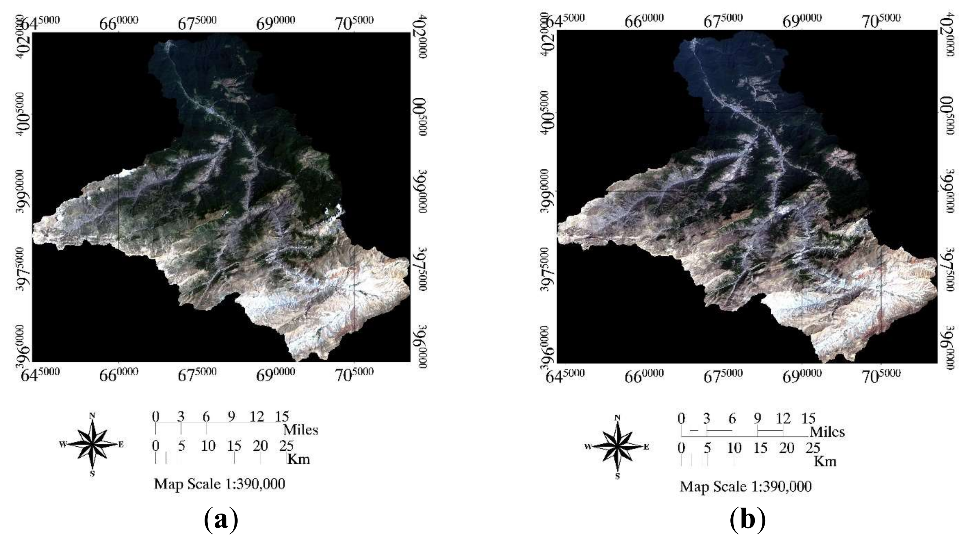
Figure 2.
Satellite images (Path/Row: 163/35) (a) 9 June 1991 and (b) 10 June 2013.

Figure 3.
Flowchart for creation of land use scenarios and SWAT simulation.

Figure 4.
Land use maps for Talar watershed in 1991 and 2013.

Figure 5.
Land-use scenario in 2050.

Figure 6.
Hydrographs of observed and simulated monthly flow at Shirgah (A); Kerikkola (B) and Polseffid (C) stations during 2001–2008 (calibration period) and 2009–2012 (validation period).
Figure 6.
Hydrographs of observed and simulated monthly flow at Shirgah (A); Kerikkola (B) and Polseffid (C) stations during 2001–2008 (calibration period) and 2009–2012 (validation period).


Figure 7.
Observed and simulated monthly nitrate load for calibration and validation periods during 2012–2013 passing through the cross-section of Shirgah station.
Figure 7.
Observed and simulated monthly nitrate load for calibration and validation periods during 2012–2013 passing through the cross-section of Shirgah station.

Figure 8.
Changes in average annual discharge yield in sub-basins for three land use scenarios (S1, S2 and S3).
Figure 8.
Changes in average annual discharge yield in sub-basins for three land use scenarios (S1, S2 and S3).

Figure 9.
Changes in average annual nitrate load in sub-basin for three land use scenarios (S1, S2 and S3).
Figure 9.
Changes in average annual nitrate load in sub-basin for three land use scenarios (S1, S2 and S3).


Table 1.
Model inputs and data sources for the studied watershed.
| Data | Data Item | Station | Data Period | Sources |
|---|---|---|---|---|
| Weather data | Precipitation Max./Min. Temperature Solar radiation Wind speed | Gharakheil, Polsefid, | 2000–2013 | Iran meteorological organization |
| Relative humidity | Allasht (Synoptic stations) | |||
| Hydrological data (measured daily) | Discharge | Shirgah, Kerikola, Polsefid, | 2000–2013 | Iran Water Resources Management Company |
| Water quality data | Nitrate | Shirgah | 2012–2013 | Iran Water Resources Management Company |
| Soil map | Soil physical and chemical properties | - | 2008 | Forests, Range and Watershed Management. IR of Iran |
| Land use | Satellite images (Landsat) | - | 1991–2013 | http://earthexplorer.usgs.gov/ |
Table 2.
General performance for recommended statistics at a monthly time step [47].
Table 2.
General performance for recommended statistics at a monthly time step [47].
| Performance Rating | NSE | Percent Bias (PBIAS) | |
|---|---|---|---|
| Stream Flow | Nitrate | ||
| Very good | 0.75 < NSE < 1.00 | PBIAS < ±10 | PBIAS < ±25 |
| Good | 0.65 < NSE < 0.75 | ±10 < PBIAS < ±15 | ±25 < PBIAS < ±40 |
| Satisfactory | 0.50 < NSE < 0.65 | ±15 < PBIAS < ±25 | ±40 < PBIAS < ±70 |
| Unsatisfactory | NSE < 0.50 | PBIAS > ±25 | PBIAS > ±70 |
NSE: Nash Sutcliffe model efficiency; PBIAS: Percent Bias.
Table 3.
Error matrix and accuracy assessment of the land use map for 1991.
| Land Use | Forest | Irrigated Land | Dry Land Farming | Residential Area | Range Land | Total | Producer Accuracy (%) |
|---|---|---|---|---|---|---|---|
| Forest | 472 | 0 | 0 | 0 | 0 | 472 | 100 |
| Irrigated land | 0 | 72 | 0 | 0 | 0 | 72 | 100 |
| Dryland farming | 0 | 0 | 23 | 0 | 4 | 27 | 85.2 |
| Residential Area | 0 | 0 | 0 | 42 | 27 | 69 | 60.9 |
| Range land | 0 | 0 | 0 | 0 | 297 | 297 | 100 |
| Total | 472 | 72 | 23 | 42 | 328 | 937 | - |
| Overall accuracy = 96.69% and Kappa index = 0.94. | |||||||
Table 4.
Error matrix and accuracy assessment of the land use map for 2013.
| Land Use | Forest | Range Land | Irrigated Land | Dry Land Farming | Residential Area | Total | Producer Accuracy (%) |
|---|---|---|---|---|---|---|---|
| Forest | 1257 | 0 | 0 | 0 | 0 | 1257 | 100 |
| Range land | 2 | 987 | 0 | 0 | 0 | 990 | 99.8 |
| Irrigated land | 0 | 0 | 80 | 0 | 0 | 80 | 100 |
| Dry land farming | 7 | 357 | 5 | 116 | 13 | 498 | 23.3 |
| Residential area | 0 | 0 | 2 | 0 | 179 | 181 | 98.9 |
| Total | 1266 | 1345 | 87 | 116 | 192 | 3006 | 100 |
| Overall accuracy = 87.15% and Kappa index = 0.80. | |||||||
Table 5.
Land use changes between 1991 and 2013.
| Land Use | 1991 | 2013 | Change | |||
|---|---|---|---|---|---|---|
| Area (%) | Area (ha) | Area (%) | Area (ha) | Area (%) | Area (ha) | |
| Forest | 40.8 | 83,902.75 | 34.8 | 71,424.71 | −14.9 | −12,478.04 |
| Irrigated land | 0.5 | 1017.82 | 0.7 | 1493.82 | +46.8 | +476 |
| Dry land farming | 11.3 | 23,272.06 | 14.8 | 30,520.31 | +31.1 | +7248.25 |
| Range land | 46.6 | 95,826.45 | 48.8 | 10,0307.5 | +4.7 | +4481.05 |
| Residential area | 0.8 | 1563.77 | 0.9 | 1837.72 | +17.5 | +273.95 |
Table 6.
Land use changes from 1991 to 2013 and the 2050 scenario.
| Land-Use Type | Land-Use 1991 (ha) | Land-Use 2013 (ha) | Change (1991–2013) | Change Annual Rate (ha) | Scenario 2050 (ha) | Change (1991–2050) |
|---|---|---|---|---|---|---|
| Forest | 83,902.75 | 71,424.71 | −12,478.04 | −542.52 | 51,351.47 | −32,551.28 |
| Irrigated land | 1017.82 | 1493.82 | +476 | +20.70 | 2259.72 | +1241.90 |
| Dry land farming | 23,272.06 | 30,520.31 | +7248.25 | +315.14 | 42,180.49 | +18,908.43 |
| Range land | 95,826.45 | 100,307.5 | +4481.07 | +194.83 | 107,516.21 | +11,689.76 |
| Residential Area | 1563.77 | 1837.72 | +273.95 | +11.91 | 2278.39 | +714.62 |
Table 7.
SWAT parameters that were fitted and their final calibrated values.
| Sensitive Parameters | Definition | Final Parameter Value |
|---|---|---|
| CN2 | SCS runoff curve number for moisture condition II | 0.57 |
| SMTMP | Snow melt base temperature | −2.09 |
| SOL_BD | Moist bulk density | −0.32 |
| SFTMP | Snowfall temperature | 8.68 |
| ALPHA_BNK | Base flow alpha factor for bank storage | 0.11 |
| SOL_K | Soil hydraulic conductivity | 0.51 |
| SMFMN | Melt factor for snow in December 21 | 1.73 |
| SOL_AWC | Soil available water storage capacity | 0.05 |
| SLSUBBSN | Average slope length | 1.81 |
| REVAPMN | Threshold depth of water in the shallow aquifer for “revap” to occur | 249.23 |
| LAT_TTIME | Lateral flow travel time | −15.50 |
| CANMX | Maximum canopy storage | 34.93 |
| TIMP | Snow pack temperature lag factor | 0.92 |
| CH_N2 | Manning’s “n” value for the main channel | 0.52 |
| GWQMN | Threshold depth of water in the shallow aquifer required for return flow to occur | 3652.82 |
| SURLAG | Surface runoff lag time | 0.78 |
| TLAPS | Temperature lapse rate | 67.63 |
| ESCO | Outflow simulation option | 0.47 |
| GW_REVAP | Groundwater “revap” coefficient | 0.12 |
| ALPHA_BF | Baseflow alpha factor | −0.42 |
| SDNCO | Denitrification threshold water content | 0.50 |
| ERORGN | Organic N enrichment ratio for loading with sediment | 0.94 |
| SOL_NO3 | Initial NO3 concentration in the soil layer | 25.69 |
| SOL_ORGN | Initial organic N concentration in the soil layer | 75.09 |
Table 8.
Model statistical evaluation for monthly flow and nitrate load for 2006.
| Item | Station | Period | Mean | NSE | R2 | PBIAS | |
|---|---|---|---|---|---|---|---|
| Observed | Simulated | ||||||
| Streamflow | Shirgah | Calibration | 4.83 | 4.72 | 0.67 | 0.68 | 4.2 |
| Validation | 5.01 | 5.19 | 0.62 | 0.65 | 5.3 | ||
| Kerikkola | Calibration | 1.86 | 1.98 | 0.57 | 0.63 | 6.2 | |
| Validation | 1.48 | 1.70 | 0.71 | 0.75 | 13 | ||
| Polseffid | Calibration | 2.25 | 2.43 | 0.60 | 0.62 | 7.4 | |
| Validation | 2.02 | 2.08 | 0.75 | 0.76 | 1.3 | ||
| Nitrate load | Shirgah | Calibration | 30,116.8 | 31,850 | 0.74 | 0.75 | 5.4 |
| Validation | 27,924.1 | 19,762.33 | 0.62 | 0.83 | −39.3 | ||
Table 9.
Percent changes in simulated average annual discharge and nitrate transport for three land use scenarios (S1: 1991, S2: 2013 and S3: 2050).
Table 9.
Percent changes in simulated average annual discharge and nitrate transport for three land use scenarios (S1: 1991, S2: 2013 and S3: 2050).
| Sub-Basin | Discharge Change (%) | Nitrate Change (%) | ||||
|---|---|---|---|---|---|---|
| S1-S2 | S2-S3 | S1-S3 | S1-S2 | S2-S3 | S1-S3 | |
| 1 | +21.4 | +43.6 | +74.4 | +18.2 | +163.8 | +211.9 |
| 2 | +13.2 | +883.5 | +1013 | +2.9 | +4 | +7 |
| 3 | 0 | 0 | 0 | 0 | +846 | +846 |
| 4 | +27.8 | +43.3 | +83.2 | +23.6 | +210.6 | +283.9 |
| 5 | +32.5 | +56.2 | +107.0 | +31.9 | +73.7 | +129.1 |
| 6 | +69.1 | +53.1 | +158.9 | +10.2 | +470.4 | +528.5 |
| 7 | +4.2 | +899.6 | +941.8 | +3.2 | −20.8 | −18.3 |
| 8 | 0 | +0.4 | +41.7 | 0 | +300.2 | +300.2 |
| 9 | +84.6 | +49.7 | +176.2 | +11.8 | +512 | +626.9 |
| 10 | +60.5 | +51.3 | +142.8 | +36.8 | +568 | +813.7 |
| 11 | +3.8 | +99.0 | +106.6 | +32.8 | −5.8 | +25.1 |
| 12 | +81.3 | +19.5 | +116.6 | +126.6 | +661.9 | +1626.5 |
| 13 | +197.9 | 0 | +197.9 | +613.5 | 0 | +613.5 |
| 14 | +241.9 | +20.4 | +311.7 | +74.2 | +1968.7 | +2469.1 |
| 15 | +229.4 | +24.6 | +310.4 | +11.4 | +1277.6 | +1433.8 |
| 16 | +3.6 | +11.9 | +404.4 | −1.8 | +1240.5 | +1216 |
| 17 | +1.2 | +19.8 | +147 | +294.8 | +1087.3 | +4587.8 |
| 18 | +62.7 | +14.3 | +85.9 | +115.2 | +817.4 | +1873.9 |
| 19 | +43.2 | +8.7 | +55.6 | +250.3 | +1000.8 | +3767.4 |
| 20 | +47.9 | +8.7 | +60.8 | +257.3 | +809.8 | +3151.1 |
| 21 | 0 | +0.6 | +56.9 | +514.9 | +6.1 | +551.9 |
| 22 | +936.6 | +6.2 | +1001.2 | +80.1 | +452.4 | +894.9 |
| 23 | +37.5 | +6.8 | +46.8 | +106.7 | +3820.7 | +8003.2 |
© 2018 by the authors. Licensee MDPI, Basel, Switzerland. This article is an open access article distributed under the terms and conditions of the Creative Commons Attribution (CC BY) license (http://creativecommons.org/licenses/by/4.0/).
Share and Cite
MDPI and ACS Style
Kavian, A.; Mohammadi, M.; Gholami, L.; Rodrigo-Comino, J. Assessment of the Spatiotemporal Effects of Land Use Changes on Runoff and Nitrate Loads in the Talar River. Water 2018, 10, 445. https://doi.org/10.3390/w10040445
AMA Style
Kavian A, Mohammadi M, Gholami L, Rodrigo-Comino J. Assessment of the Spatiotemporal Effects of Land Use Changes on Runoff and Nitrate Loads in the Talar River. Water. 2018; 10(4):445. https://doi.org/10.3390/w10040445
Chicago/Turabian StyleKavian, Ataollah, Maziar Mohammadi, Leila Gholami, and Jesús Rodrigo-Comino. 2018. "Assessment of the Spatiotemporal Effects of Land Use Changes on Runoff and Nitrate Loads in the Talar River" Water 10, no. 4: 445. https://doi.org/10.3390/w10040445
Note that from the first issue of 2016, this journal uses article numbers instead of page numbers. See further details here.