Article

What Large Sample Size Is Sufficient for Hydrologic Frequency Analysis?—A Rational Argument for a 30-Year Hydrologic Sample Size in Water Resources Management

1
Key Laboratory of Groundwater Resources and Environment, Ministry of Education, Jilin University, Changchun 130021, China
2
Department of Hydrology & Water Resources Engineering, Chang’an University, Xi’an 710054, China
3
Institute of water resources and hydro-electric engineering, Xi’an University of Technology, Xi’an 710054, China
4
Department of Civil Engineering, Chungnam National University, Daejeon 34134, Korea
5
International Water Resources Research Institute, Chungnam National University, Daejeon 34134, Korea
6
Yunqing Xuan, College of Engineering, Swansea University, Swansea SA2 8PP, UK
7
Nanjing Hydraulic Research Institute, State Key Laboratory of Hydrology-Water Resources and Hydraulic Engineering, Nanjing 210029, China
8
Research Center for Climate Change, Ministry of Water Resources, Nanjing 210029, China
*
Author to whom correspondence should be addressed.
Water 2018, 10(4), 430; https://doi.org/10.3390/w10040430
Submission received: 4 February 2018 / Revised: 27 March 2018 / Accepted: 2 April 2018 / Published: 4 April 2018

Abstract

:
The calculation of hydrologic frequency is an important basic step in the planning and design stage of any water conservancy project. The purpose of the frequency analysis is to deduce the hydrologic variables under different guarantee rates, and to provide hydrologic information for water conservancy project planning and design. The calculation of hydrologic frequency requires that the sample size is large enough, as only then can the statistical characteristics of samples take the place of the total statistical eigenvalues. This means that the samples can reveal the statistical characteristics of hydrologic variables and identify the randomness rule of hydrologic phenomena. Many countries in the East Asian monsoon climate zone (China, Japan and South Korea) have stipulated a sample size of 30 years for hydrologic frequency analysis. In this paper the rationality of the 30-year sample size is proved by analyzing the periodic and random rules of hydrologic phenomenon and the influencing mechanism of solar activity, and by adopting the general conclusion of the sampling theorem. Then, using the wavelet analysis method to examine annual precipitation data in a long series generated from representative precipitation observation stations in China, the strong-weak cycle of solar activity is proved to be 10 years, which is consistent with the wet-dry cycle of the representative precipitation stations (10–12 years). Finally, adopting numerical modeling to analyze the normal distribution of randomly generated samples and long-range annual precipitation data collected from representative stations, hypothesis testing (u, F and t) is used to prove that a 30-year sample size is reasonable. This research provides a reference as to how to prove the necessary sample size for relevant statistical analyses (for example, how large the sample should be for analyzing hydrologic factors trend evolution, hydrologic data consistency and ergodicity of statistical samples), thus ensuring the reliability of the analytical results.

1. Introduction

A great variety of factors affect the hydrologic circulation of a river basin, and no single factor is absolutely dominating; hence, the hydrologic phenomenon takes on randomness [1]. Frequency of occurrence is adopted in the hydrologic field to describe the occurrence probability of hydrologic variables. For instance, among long-range annual observed precipitation data, the occurrences of a wet year and a dry year are fewer and the volume of runoff is close to the average value. Hydrologic frequency refers to the number of occurrences that a hydrologic variable equals or exceeds a certain value. For example, frequencies of 1%, 50% and 95% typically indicate a wet year, average year and dry year, respectively.
Hydrologic frequency analysis is used to calculate the hydrologic variable design value xp as it is responsive to design frequency p based on long-range historical observation data. The method involves fitting the probability distribution function of the hydrologic variable based on the statistical characteristic value (x, Cv and Cs) of the hydrologic variable. The limit theorem [2] shows that the noticeable statistical nature of the random phenomenon can be revealed via a number of repeated experiments. The large number theorem [3] proves that when the experiment is repeated a sufficient number of times, the sampled average value will be close to the overall average value. The central limit theorem [4] proves that if a random variable is generated by the combined influence of a great many independent random factors, and each factor by itself exerts only minimal influence (i.e., no dominating factor), then the generated random variable can be deemed as the sum of multiple random variables. Furthermore, when the sample size is large enough, the random variable can be shown to follow or almost follow a normal distribution. In summary, for hydrologic frequency analysis, so long as the sample size is large enough, the distribution function of the hydrologic variables for a river basin can be determined using statistical rules.
Hydrologists in all countries establish the practical standard for hydrologic frequency calculations based on probability theory combined with regional hydrologic experiences. For example, China requires a sample size of 30 years [1] and a P-III type of distribution [5]; Korea requires a sample size of 30 years, a Gumbel distribution and a Wakeby distribution [6,7]; Japan requires a sample size of the most recent 30 years [8]; Zimbabwe uses a 30-year sample size [9], and the Nyanyadzi River uses historical runoff data and the Gumbel distribution to calculate the once-in-every-200 years wet year (0.5%). The calculation of runoff frequency in the United Kingdom [10] adopts a generalized logistic distribution, which is a probability function close to the P-III distribution, and the calculation of rainfall frequency uses a Gumbel distribution and requires a sample size that is four times the return period. For example, determining a once-in-20 years wet year (5%) entails a sample size of 80 years.
The United Kingdom is located near the Atlantic Ocean and belongs to the temperate marine climate zone that is warm and humid in winter, warm and wet in summer, and has evenly distributed inter-annual precipitation during the year; furthermore, the designed wet frequency is generally low. Differences in hydrologic and climatic conditions also determine the size requirements of water samples. For example, in China where the East Asian monsoon prevails, the inter-annual variability in precipitation caused by the strength of monsoons is large, and serious droughts and floods occur frequently. If the United Kingdom’s method of determining sample size were adopted for designing water conservancy projects in China with a wet control standard for once-in-100 years (1%), the frequency calculation would require a sample size of 400 years, which is obviously not realistic.
The theory of probability requires that the hydrologic variable sample size should be large enough to ensure the statistical characteristics of samples approximate that of the entire population. Based on a large number of regional experiences, hydrologists of the East Asian monsoon climatic region require a data period of 30 consecutive years for hydrologic frequency analysis. This paper proves the rationality of the 30-year sample size from the aspects of physical analysis and numerical simulation.

2. Physical Mechanism that Restricts the Sample Size

2.1. The Law of Solar Activities Makes the Hydrologic Phenomenon almost Periodic

The climate characteristics in a river basin are mainly affected by solar activities, atmospheric circulation, the natural geographical environment and other factors. As summarized elsewhere [11], the effect of solar radiation is an astronomical factor that is beyond the hydrologic cycle system, and has a periodic influence on climate. Atmospheric circulation is the dominant factor affecting climate, and takes on a seasonally changing trend. Meanwhile, the effects of various factors are to be realized by affecting the atmospheric circulation, which means that atmospheric circulation provides the basic conditions for various activities of the weather system and takes on a random nature. The natural geographical features of a basin have consistent effects on atmospheric circulation, which reflects the particularity and consistency of the basin response. Therefore, the hydrologic climate of a basin is a coupled superposition of periodic and stochastic laws, showing regularity on a long timescale and randomness on a short timescale.
Research [12] shows that the wet and dry runoff changes of China’s second Songhua River basin are affected by the solar cycle, also known as the solar magnetic activity cycle, a quasi-periodic change of sunspot number and other phenomena with an approximate period of 11 years. Further studies [11] show that the abnormal years with serious wet periods and drought for basin runoff are periodic; for instance, the serious drought and wet periods in the Nenjiang River and the second Songhua River in China are almost periodic at 10-year cycles, with a 1-year error.

2.2. Sampling Theory Serving as Theoretical Basis for Sample Size

Sampling theory [13,14], also known as Nyquist theory, was proposed by American telecommunication engineer Harry Nyquist in 1928 and defines the sufficient conditions for sampling frequency. In the original application, sampling frequency allowed a discrete sampling sequence to capture all information from limited continuous time signals. In the field of digital signal processing, a continuous time signal is usually called an “analog signal”, and a discrete time signal is usually referred to as “digital signal”. In the process of simulation and conversion of digital signals, when the sampling frequency is twice the highest frequency of the signal, the digital signal after sampling can completely preserve the original signal information. In general practice, the signal sampling frequency should be 2.5–4 times the highest frequency of the signal.
In 1933, V. A. Kotelnikov, a Soviet engineer, used the sampling frequency algorithm to give a rigorous expression of this theorem for the first time; hence it was called the V. A. Kotelnikov sampling theorem in the Soviet Union’s literature. In 1948, C. E. Shannon, founder of information theory, gave a clear account of the Kotelnikov’s procedure and formally quoted it as a theorem. Therefore, it is also called the Shannon sampling theorem in most literature.
The sampling theorem can be expressed in a variety of ways, and the most basic ones are the time domain sampling theorem and the frequency domain sampling theorem. The time domain sampling theorem is the foundation of sampling error theory, random variable sampling theory and multivariate sampling theory.
Obviously, the rules of hydrologic variables expression are affected by the solar activity cycle. According to the sampling theorem, the sample size of hydrologic phenomena for statistical regularity should be (10–11) × 2.5 = 25–27.5 years, thus proving from a physical mechanism that a 30-year sample size is appropriate for hydrologic frequency calculations.

3. Characteristics of Hydroclimate in China

Precipitation is not only the basic link of the hydrologic cycle but also the basic element of the water balance. It is both the original source of surface runoff and the main source of groundwater recharge; moreover, it is also an important index that reflects the characteristics of regional hydrology and climate. The uneven and unstable spatial and temporal distribution of precipitation is the direct cause of flooding and drought in China. For the analysis that follows, six representative precipitation observation stations (Figure 1) were selected as the sites for precipitation data. The precipitation characteristics of the six representative precipitation stations are described (see Table 1).

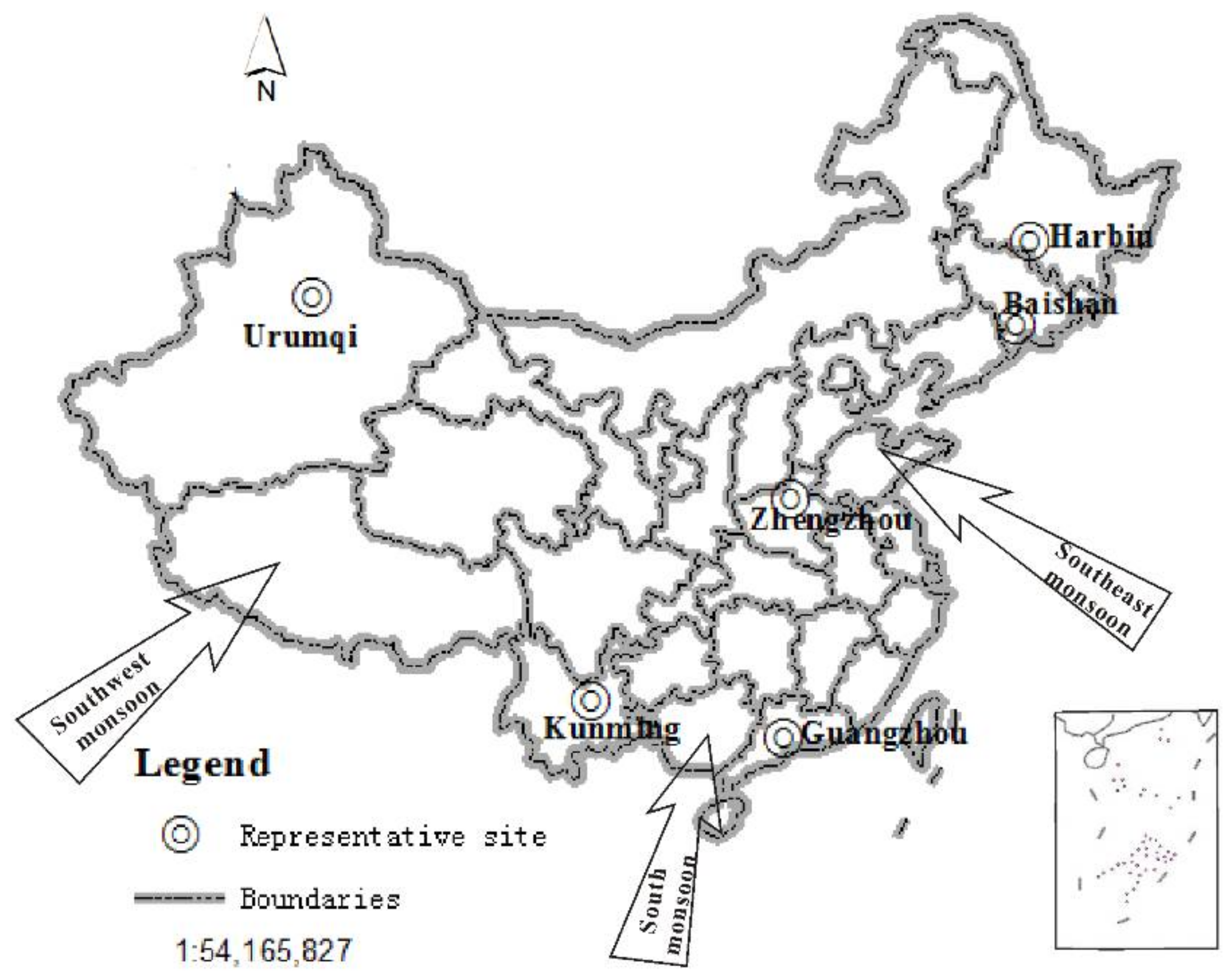
3.1. Analysis of Water Vapor Sources for China

Located in the eastern part of Eurasia and the west side of the Pacific Ocean, China is in the interaction zone between the oceanic and the continental airflow fields; thus, it is one of the countries with the most conspicuous features of a monsoon climate [15]. As shown in Figure 1, the southwest monsoon from the Pacific Ocean affects the vast eastern region of China, while the southwest monsoon from the Indian Ocean and the South China Sea mainly affects the coastal areas of southwest and south China. Thus, approximately 67% of the Chinese territory is a monsoon-influenced area. In the summer, easterly wind has difficulty reaching the northwest hinterland of China as this region is far from the oceans and is screened by mountains and plateaus. Therefore, Chinese precipitation mainly comes from the southeast corridor along the south of the subtropical high pressure zone of the Pacific Ocean, the southwest corridor along the Indian Ocean via the Bay of Bengal [16,17,18], as well as a weakly northwest corridor via the westerly circulation [19]. These three corridors reflect the influences on China’s precipitation by the southeast monsoon, southwest monsoon and mid-latitude northwest wind, respectively [20].

3.2. Regional Precipitation Cycle Identification

The temporal and spatial distributions of river runoff and precipitation are generally overlapping [21]. Furthermore, regional precipitation is not significantly affected by human activities and is stable over a long timescale. Therefore, the statistical characteristics of regional precipitation are used to reveal the regularity of inter-annual water resources evolution in order to argue the sufficiency of sample size for flood frequency calculations.
The wavelet analysis method [22] was adopted for cycle identification. Morlet wavelet analysis has the function of time-frequency multi-resolution, which can accurately identify the varying period of changes hidden in a time sequence. The isoline map of wavelet coefficients can reflect the periodic variations of different timescales in the time sequence and the responsive distribution in the time domain. In an isoline map of wavelet coefficients, the X-axis of the ordinate indicates the time (year) while the Y-axis indicates the time scale, and the isoline shows the value of wavelet coefficients. The visual portrayal of scale-based wavelet variance is called a wavelet variance graph, which can reflect the distribution of scaled-based changes of random variables. Therefore, the wavelet variance graph can be used to identify the relative intensity and the main timescale, or main cycle of different scale disturbances among random variables. Figure 2 shows the structure of the wavelet in the relative number sequence of sunspots, and Figure 3 reveals the result of wavelet analysis of precipitation from the six representative regional stations in China.
Table 2 shows the results of the statistical analysis of wavelet variance based on Figure 2 and Figure 3, from which it can be seen that the sunspot activity is periodic with a cycle of 9–12 years, and corresponds with general knowledge about the 11-year cycle of solar activity. The high and low changes of precipitation at representative stations are periodic with a cycle of 10–12 years, which proves that the cycle of high and low changes of Chinese regional precipitations is consistent with that of the weak and strong changes of solar activities.

4. Numerical Simulation Verification

In the preceding sections of this paper, it was demonstrated that solar activity makes the hydrologic phenomena almost periodic and that the sampling theorem serves as the basis for the sampling frequency and sample size. It was also proved based on the physical mechanism that hydrologic frequency calculations require a sample size of 30 years. In this section the correctness of this inference is verified using numerical simulation experiments.
The numerical simulation experiment adopts the standard normal distribution function and the P-III function. It is worth explaining that the P-III function is the distribution function of standard sampling for hydrologic frequency calculations in China. Numerical simulation using the P-III function verifies that as the sample size increases, statistical parameters of samples tend to stabilize. In this way, the sample size for describing the distribution function is confirmed.
Karl Pearson, a British bio-statistician, studied numerous observation data from 1895 to 1916 and discovered that the frequency distribution of many random variables registers a single peak in a bell-shape function, with the frequency on both sides of the peak gradually decreasing and eventually tending to the transverse axis tangent. The differential equation describing the distribution is:
d y d x = ( x + d ) y b 0 + b 1 x + b 2 x 2
In Equation (1), y = p(x) is the probability density. The origin of the coordinate is located at x, the mean value of the variable; d is the distance between the maximum and the mean, and b0, b1 and b2 are parameters.
According to the values of b0, b1 and b2, and the root of b0 + b1x + b2x2 = 0, 13 different density functions can be attained after integration of Equation (1) to form a Pearson curve cluster; the normal distribution and P-III distribution are two curve types in the cluster.
Equation (2) is an over-limit normal distribution function,
G ( x ) = 1 2 π x e x 2 2 d x ,   0 < x <
After 1924 when Forster [23] for the first time applied the P-III distribution function in hydrologic phenomena analysis, it became widely used by hydrologists everywhere and has been incorporated into the hydrologic frequency calculation specification of many countries such as China, South Korea, Thailand, Austria, Bulgaria, Hungary, Poland, Romania and Switzerland.
Equation (3) is an over-limit P-III distribution function:
G ( x ) = β α Γ ( α ) x ( x a 0 ) α 1 e β ( x a 0 ) d x ,   0 < x <
In Equation (3), α, β and a0 are the parameters of the shape, scale and position of the P-III distribution function, respectively, and can be attained via statistical calculations as follows.
α = 4 C s 2
β = 2 x ¯ C v C s
a 0 = x ¯ ( 1 2 C v C s )
In Equations (4)–(6), Cv and Cs are the variation coefficient and skewness coefficient, respectively, which can be obtained by sample calculation. The calculation of Cv includes a cube, and the exponential function will show a geometric incremental trend and the sample noise is increased. γ = Cs/Cv, γ and Cv are usually used to calculate Cs. A value for γ can be found in a hydrologic manual; for example, the value of 2.5 is usually used for the Songhua River Basin in Northeast China.

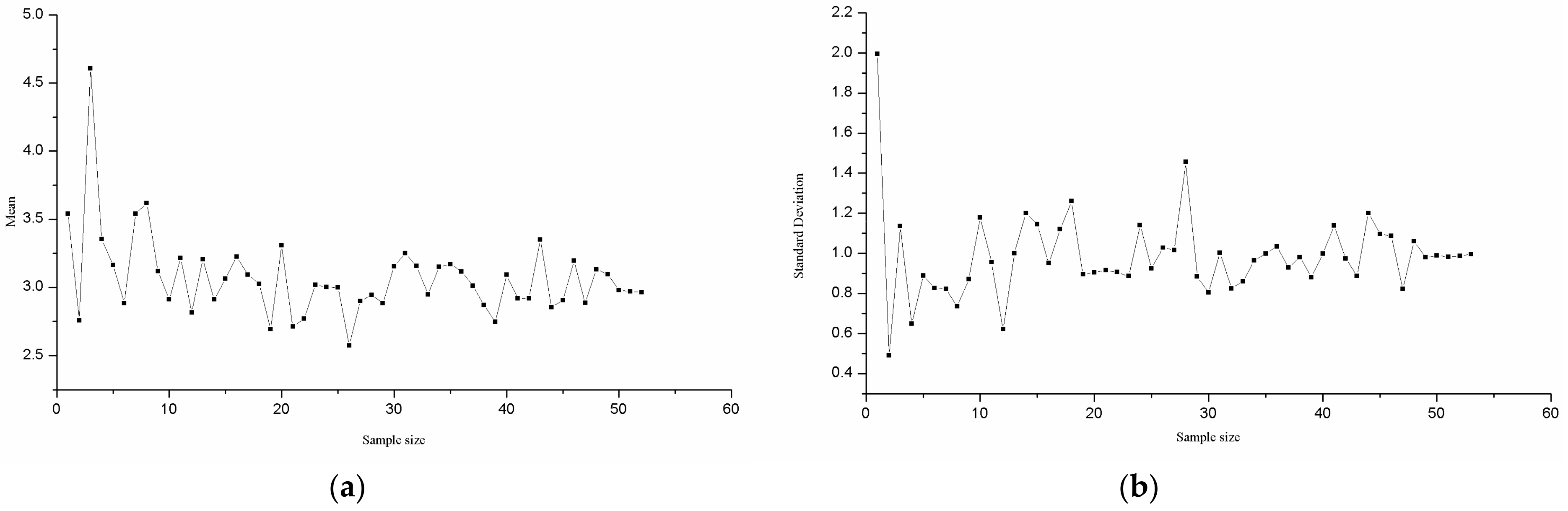
4.1. Normal Distribution Simulation

First, select the standard normal distribution as the simulation object to ensure the function value is positive. Take [G(x) + 3] to describe the distribution, for which the theoretical mean value is a0 = 3, and the theoretical mean variance is σ0 = 1. Then, the discrete sample of the normal distribution is randomly generated, and the trends of mean value x ¯ and mean variance value σ are analyzed while increasing the sample size (Figure 4). As is seen in Figure 4a, the mean value x ¯ gradually approaches 3 with increasing sample size; and as is seen in Figure 4b, the mean variance value σ gradually reaches 1 with increasing sample size.
As is shown in Figure 4a, as the sample size increases, the mean value x ¯ gradually approaches the theoretical mean value 3, which is corroborated via u hypothesis verification [24]. According to the sample sequence in Figure 4a, when the sample size equals 30, the mean value x ¯ 30 is = 3.15 and the u-statistic is:
u = x 30 ¯ a 0 σ 0 n = 3.15 3 1 30 0.84
With the degree of confidence α = 5% and by referring to a standard normal distribution, it can be calculated that uα/2 = 1.96 < u; thus, via u verification, it is proved that the calculated mean value x ¯ = 3.15 when the sample size is 30 is reasonable.
As is shown in Figure 4b, when the sample size increases, the mean variance σ gradually approaches the theoretical value of 1, which is corroborated via hypothesis F verification [25]. This test method and hypothesis testing are used to further demonstrate that, according to sample series shown in Figure 4b, when the sample size is equal to 30, the standard variance σ30 = 0.89, and the F-statistic is:
F = σ 0 2 σ 30 2 = 1 0.89 2 1.26
With v1 = n1 − 1 = 30 − 1 = 29, v2 = n2 − 1 = , and confidence degree α = 10%, the standard F distribution chart shows F0.05 = 1.342 > F, and thus, via F verification, the calculated mean variance σ = 0.89 when the sample size is 30 is reasonable.

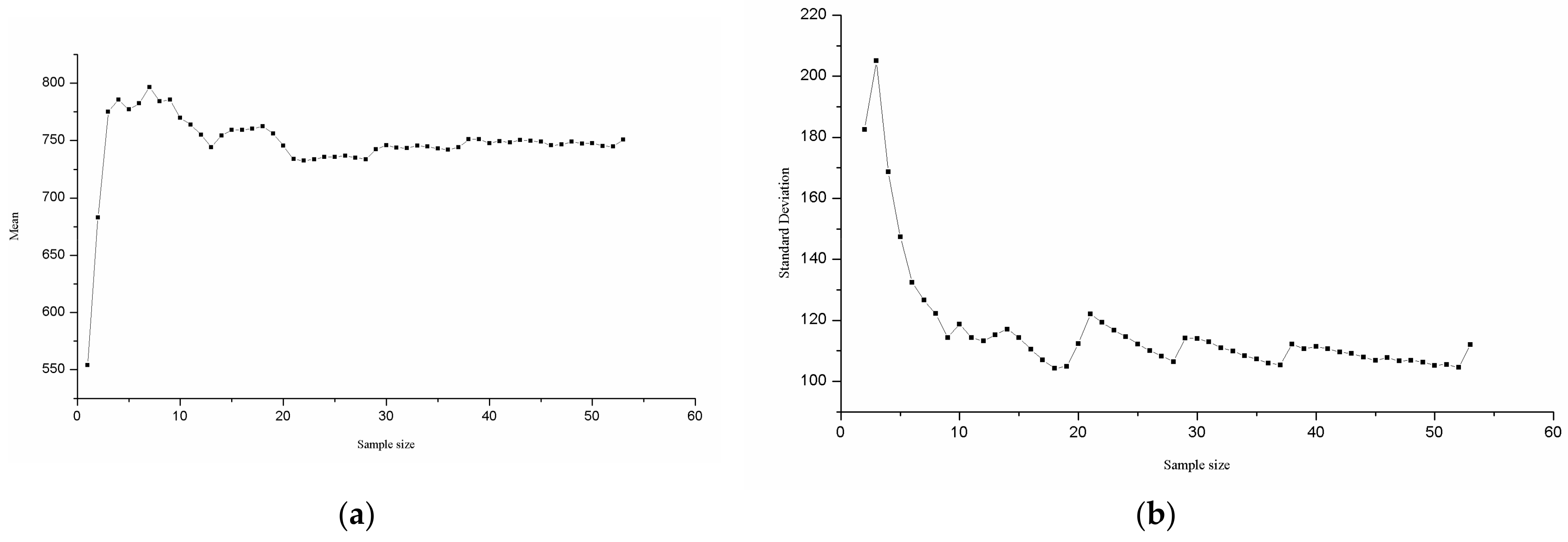
4.2. P-III Distribution

As noted previously, six representative stations in China were selected (Figure 1) to carry out the hypothesis verification of the mean and variance.
The 53-year precipitation series from 1958 to 2010 of the Baishan station in the second Songhua River basin is used as an example. In the analysis of hydrologic frequency, the P-III distribution is confirmed by three statistical parameters of the samples (mean x ¯ , the coefficient of variation Cv and Cs). Furthermore, Cv = σ/ x ¯ and Cs = γCv. By analyzing the sample mean x ¯ and the variance σ, the sample size of 30 for hydrologic frequency calculations can be proved to be reasonable. Figure 5 shows the trends of x ¯ and mean variance σ changing as sample size increases.
Figure 5 shows that with the increase of sample size, the mean value and mean variance tend to become stable. The calculated mean and variance obtained from sample sizes of 30 years and 53 years are x ¯ 30 ≈ 746, x ¯ 53 ≈ 750, σ30 ≈ 114 and σ53 ≈ 112, respectively.
As the mean value and the mean variance cannot be obtained from this calculation, t-verification [26,27] can be used to verify the rationality of the mean value, and the F-verification can be used to test the rationality of the variance.
Statistic t is:
t = x 1 ¯ x 2 ¯ n 1 σ 1 2 + n 2 σ 2 2 n 1 + n 2 2 1 n 1 + 1 n 2 = 746 750 30 114 2 + 53 112 2 30 + 53 2 1 30 + 1 53 0.18
With the distribution t(n1 + n2 − 2), t0.05 = 1.66 > t; thus, there is no difference in the mean variance calculated using sample sizes of 30 and 53 at a confidence level α = 5%.
Statistic F is:
F = σ 53 2 σ 30 2 = 112 2 114 2 0.97
Using v1 = n1 − 1= 30 − 1 = 29, v2 = n2 – 1 = 52, F0.05 = 1.342 > F from a standard F-distribution chart. Thus, there is no difference in the mean variance confidence calculated with sample sizes of 30 and 53 at a confidence level of α′ = 5%.
In these two simulations, the statistical average value was calculated from the normal distribution, and the temporal average value was attained using a P-III distribution of annual precipitation at the Baishan stations in the second Songhua River basin. The two examples show that the mean value x ¯ and coefficient of variation Cv are stable when the sample size reaches 30. Hence, the numerical simulations verify that a 30-year sample size is sufficient for hydrologic frequency calculations.
Similarly, Figure 6 shows the changing trend of statistical parameters according to the increasing sizes of random samples from the annual precipitation sequences at the other five representative precipitation stations, and the hypothesis verification results are shown in Table 3.
Using the t(n1 + n2 − 2) distribution, t0.05 = 1.65 > t ; therefore, there is no difference (at a confidence level of α = 5%) in the mean calculated using sample sizes of 30 and 62 at the Harbin, Zhengzhou, Kunming and Guangzhou stations. Furthermore, with v1 = n1 − 1 = 30 − 1 = 29, v2 = n2 − 1 = 61, F0.05 = 1.649 > F according to the standard F distribution chart; thus, there is no difference (at a confidence level of α = 5%) in the mean variance calculated using sample sizes of 30 and 62 at the Harbin, Zhengzhou, Kunming and Guangzhou stations. The test results of these stations indicate that when the sample size is 30 years, the statistical parameters of the sample can accurately represent the statistical parameters of the population.
However, the Urumqi station does not pass the hypothesis verification, probably because its hydro-climatic conditions are more complex than those at the other five stations, which are all located in the southeastern and southwestern monsoon regions. In the northwest mountainous areas of Xinjiang Province of China (where the Urumqi station is located), water vapor from the Atlantic Ocean and the Arctic Ocean is the main source of precipitation. Therefore, under the influence of natural geographical conditions of this region, the inter-annual variation of precipitation is obviously different from that of areas influenced by monsoon climate.

5. Conclusions

5.1. Conclusions

In this paper the stochastic characteristics of hydrologic variables were discussed and the experiences in countries influenced by the East Asian monsoon climate were shown to require a sample size of 30 years for hydrologic frequency calculations. Then, the rationality of a 30-year sample size was demonstrated based on the periodic influence of solar activity on the hydrologic process. This was accomplished using general sampling theory, identification of the consistency between the strong-and-weak cycle of the solar activity and the wet-and-dry cycle of precipitation at representative stations, as well as statistical parameter trend analysis of the annual precipitation series from representative precipitation stations. The following conclusions are justified by the results of these analyses.
(1)
Countries in the East Asian monsoon region such as China, Japan and South Korea all require a sample size of exceeding 30 years in the calculation of hydrologic frequency.
(2)
Solar activity makes hydrologic phenomena almost periodic, and the sampling theorem can be used as a theoretical basis to deduce a reasonable sample size for hydrologic frequency calculations.
(3)
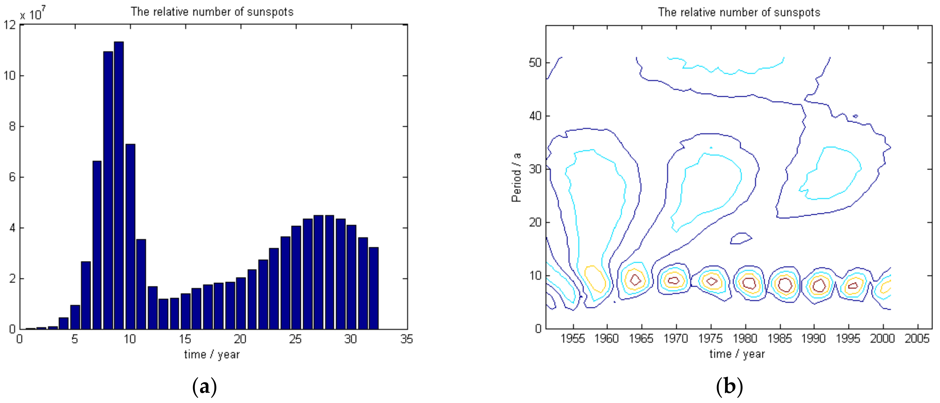
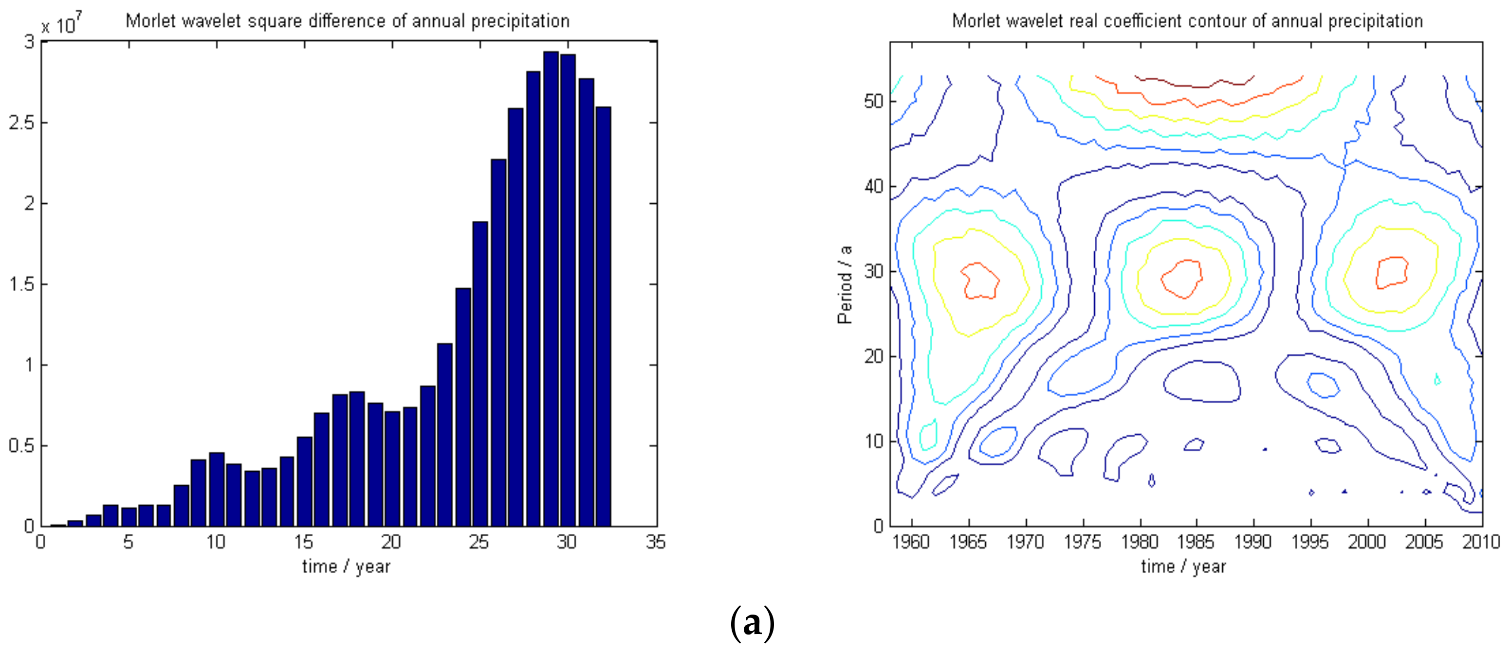
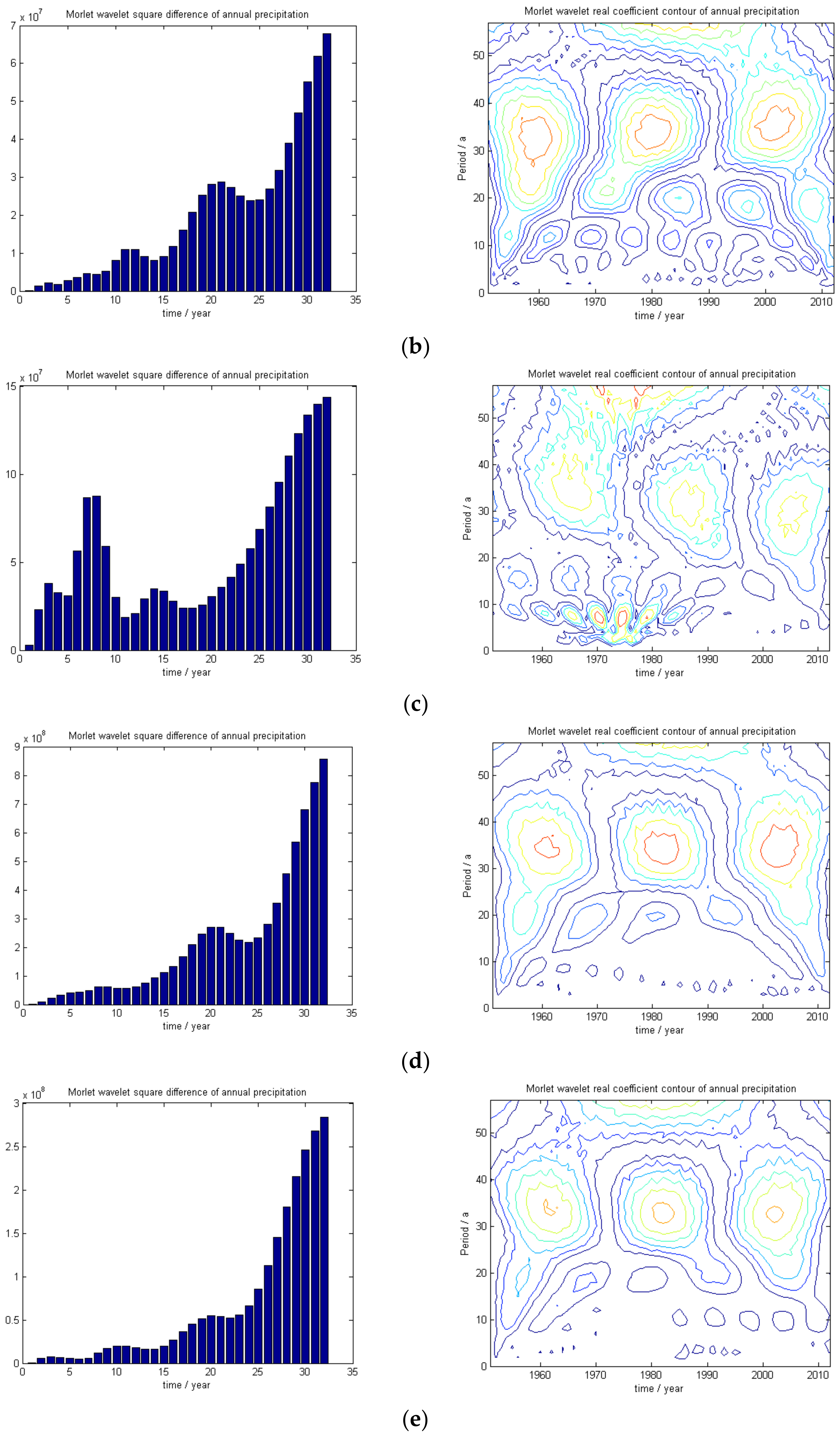
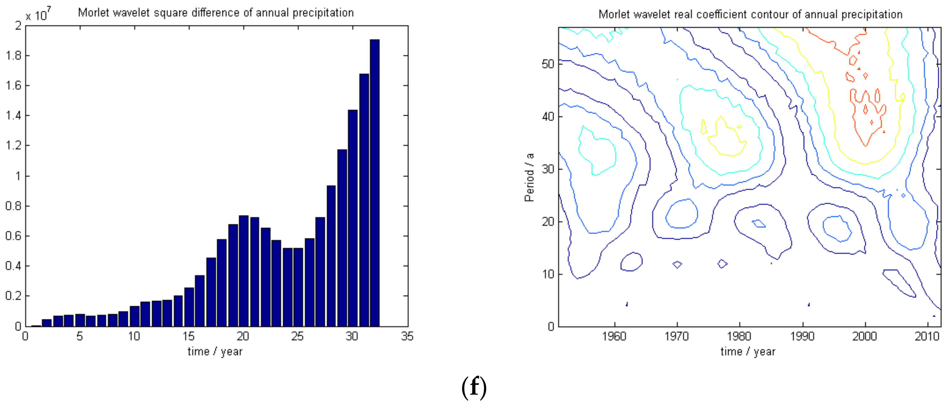
The wavelet analysis method combined with a long series of sunspot number data and representative station annual precipitation data can be used to show that solar activity is periodic with a cycle of 10 years, that the annual wet-dry cycle of representative precipitation observation stations is periodic with a cycle of 10–12 years, and that the sunspot and precipitation data are consistently aligned.
(4)
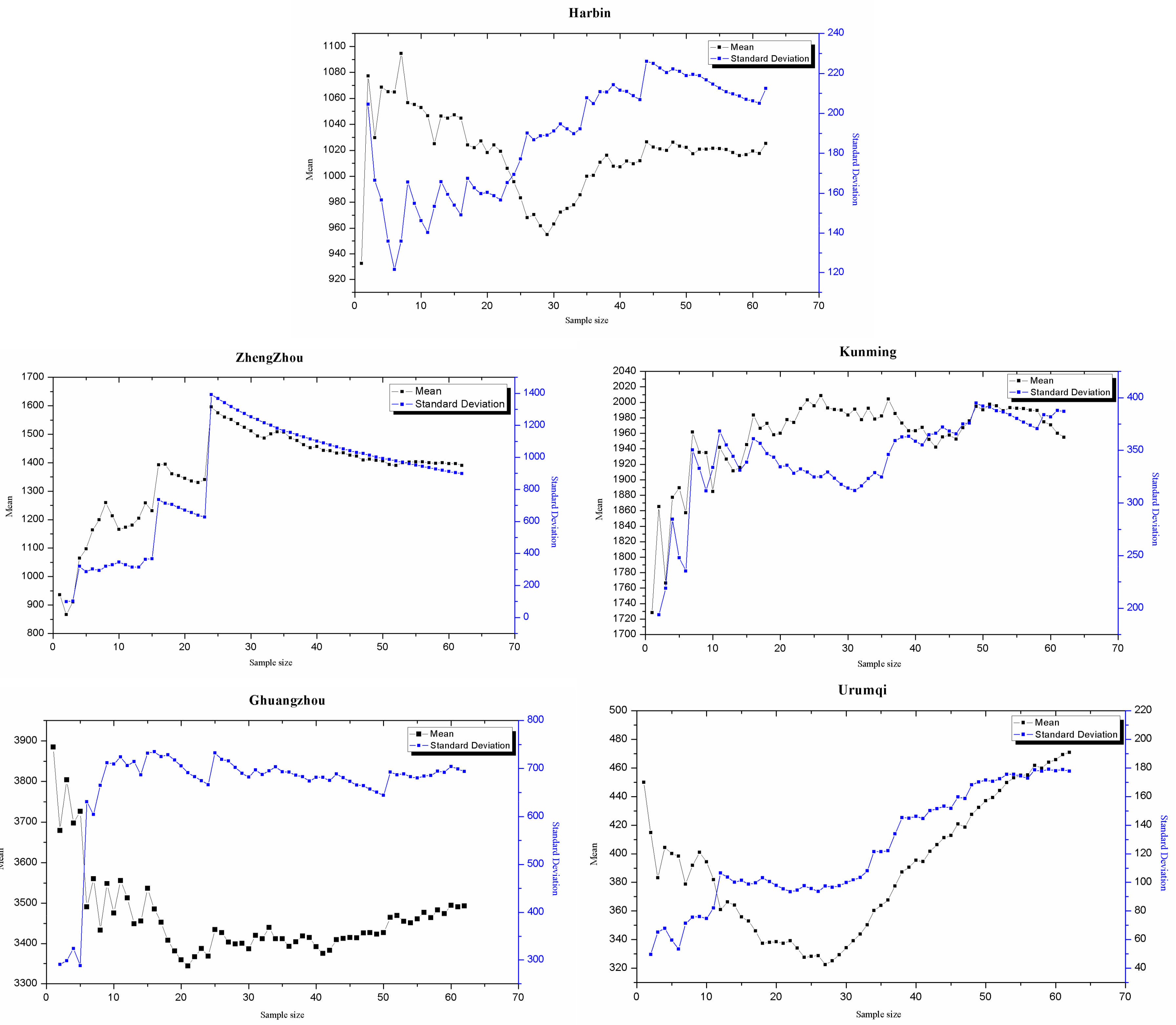
Numerical simulation of the normal distribution and the annual precipitation series of representative stations, corroborated by hypothesis verification, shows that when the sample size is 30 years, the mean and variance tend to be stable, proving that a sample size of 30 years is reasonable for the calculation of hydrologic frequency.
(5)
Precipitation data from five stations in the southeast and southwest monsoon areas of China are consistent, and statistical parameters (mean and variance) calculated using a sample size of 30 years pass the hypothesis verification test. Precipitation data from a sixth station located in the inland west wind circulation of China do not pass a hypothesis test that a 30-year sample size is adequate for hydrologic frequency calculations.
In global terms, China, Japan and South Korea (which are located in the East Asian monsoon region) require a sample size exceeding 30 years for hydrologic frequency calculations, while the for sample size requirement in other countries (such as the United Kingdom) is based on a different standard. From these arguments, we can conclude that the influence on solar activity and atmospheric circulation by natural geographical features in basins isconsistent, which also shows the particularity and consistency of basin-based responses, the same meaning is stated in the literature [11] that “the laws affecting runoff can be summarized into three categories. (1) Periodic law considers the effects that can be repeated in cycles. These are normally astronomical factors; (2) Random law includes the factors that can be subject to random effects, mainly atmospheric circulation; (3) Basin-wide law is affected by basin-wide factors, mainly underlying surface characteristics”.

5.2. Forecast

(1)
This paper aimed to provide a general method for statistical analysis to determine the reasonable sample size for hydrologic frequency calculations. The method involves making the qualitative analysis of suitable sample size according to the main influencing factors of random variables, its rule of influence and the sampling theorem. Then, numerical experiments are used to analyze the evolution trend and stabilizing state of statistical parameters of the random variables as sample size increases, from which the reasonable sample size is initially determined. Finally, through hypothesis verification, the method demonstrates how large a sample size should be so as to ensure that no significant changes occur in the values of statistical parameters describing the sample set, thus confirming that the initially determined sample size is, in fact, the proper sample size.
(2)
The sample size rationality verification can be widely applied for statistical analyses. For example, it can be used in trend analysis of hydro-meteorological factors (climate change research), to explore the hydrologic series non-stationarity issue (ergodic verification), and in artificial neural network training (excessive training problem), among other applications. When conducting these statistical analyses, statistical parameters related to the issue have to be analyzed first, and, by means of numerical analysis, the trend of change and stabilizing status of statistical parameters can be analyzed as a function of increasing sample size. Finally, hypothesis verification can be used to determine the reasonable sample size.

Acknowledgments

The author hereby would like to express deep gratitude to the key special project of “Efficient Development and Utilization of Water Resources” (2017YFC0406005), China-ROK cooperation project (51711540299), Natural Science Foundation of Jilin Province (20180101078JC), the National Natural Science Fund (51379088) and other projects which have given support to the research of this paper.

Author Contributions

Hongyan Li proposed and demonstrated scientific problems; Jiaqi Sun performed wavelet analysis and hypothesis testing; Hongbo Zhang carried out the sample representative and analyzed regional hydrological climate characteristics; Jianfeng Zhang analyzed the application of sampling theorem in this paper; Kwnasue Jung discussed the background of Korean; Joocheol Kim provided relevant references in Korea; Yunqing Xuan provided British references; Xiaojun Wang provided regional data for China; Li Fengping directed the structure of the article.

Conflicts of Interest

The authors declare no conflict of interest.

References

  1. Wang, J. Hydrologic Statistics; Water Resources and Electric Power Press: Beijing, China, 1993; Volume 6, p. 2. (In Chinese) [Google Scholar]
  2. Bure, V.; Parilina, E. Probability Theory and Mathematical Statistics; World Scientific: Singapore, 2013; pp. 617–619. [Google Scholar]
  3. Bronshtein, I.N.; Semendyayev, K.A.; Musiol, G.; Mühlig, H. Probability Theory and Mathematical Statistics; Mir Publishers: Moscow, Russia, 1986. [Google Scholar]
  4. Ibragimov, I.A.; Zaitsev, A.Y. Probability Theory and Mathematical Statistics; World Scientific: Singapore, 1992. [Google Scholar]
  5. Standard for Hydrologic Calculation of Water Resources and Hydropower Engineering; DL/T5431-2009; China Electric Power Press: Beijing, China, 2009. (In Chinese)
  6. Oh, T.-S.; Kim, M.-S.; Moon, Y.-I.; Ahn, J.-H. An Analysis of the Characteristics in Design Rainfall According to the Data Periods. J. Korean Soc. Hazard Mitig. 2009, 9, 115–127. (In Korean) [Google Scholar]
  7. Kim, N.W.; Won, Y.S. Estimates of Regional wet Frequency in Korea. J. Korea Water Resour. Assoc. 2004, 37, 1019–1032. (In Korean) [Google Scholar] [CrossRef]
  8. Japan Meteorological Office. Japan Meteorological Office; Special Edition; Japan Meteorological Agency: Tokyo, Japan, 2017. (In Japanese)
  9. Mujere, N. Wet frequency analysis using the Gumbel distribution. Int. J. Comput. Sci. Eng. 2011, 3, 2774–2778. [Google Scholar]
  10. Robson, A.J.; Reed, D.W. Statistical procedure for wet frequency estimation. In The Wet Estimation Handbook; Centre for Ecology & Hydrology: Bailrigg, UK, 1999; Volume 3. [Google Scholar]
  11. Li, H.; Wang, Y.; Li, X. Mechanism and Forecasting Methods for Severe Droughts and wets in Songhua River Basin in China. Chin. Geogr. Sci. 2011, 21, 531–542. [Google Scholar] [CrossRef]
  12. Li, H.; Xue, L.; Wang, X. Relationship between Solar Activity and Wet/Drought Disasters of the Second Songhua River Basin. J. Water Clim. Chang. 2015, 6, 578–585. [Google Scholar]
  13. Wu, T.; Hua, H. Mechanical Vibration; Tsinghua University Press: Beijing, China, 2014. (In Chinese) [Google Scholar]
  14. Sampling Theory. Econometric 1948, 16, 69.
  15. China Water Resources and Hydropower Planning and Design Institute. China’s Water Resources and Its Development and Utilization Survey; China Water Conservancy and Hydropower Press: Beijing, China, 2014; Volume10, p. 2. (In Chinese) [Google Scholar]
  16. Murakami, T. The general circulation and water-vapor balance over the Far East during the rainy season. Geoph. Mag. 1959, 29, 131–171. [Google Scholar]
  17. Shen, R.; Luo, S.; Chen, L. Relationship between Summer Monsoon Environment and Precipitation in China. In Proceedings of the Tropical Weather Conference, Beijing, China, 3 September 1980; Science Press: Beijing, China, 1980; pp. 102–111. (In Chinese). [Google Scholar]
  18. Tao, J.; Chen, J. Water vapor source and conveying channel of rainstorm in Jianghuai region. J. Nanjing Inst. Meteorol. 1994, 4, 443–447. (In Chinese) [Google Scholar]
  19. Tian, H.; Guo, P.; Lu, W. Characteristics of summer water vapor transmission and its relationship with precipitation anomalies in China. J. Nanjing Meteorol. Coll. 2002, 4, 496–502. (In Chinese) [Google Scholar]
  20. Liu, C. Chinese Hydrology; Science Press: Beijing, China, 2014; Volume 1, p. 26. (In Chinese) [Google Scholar]
  21. Miao, R. Principles of Hydrology; China Waterpower Press: Beijing, China, 2007; p. 3. (In Chinese) [Google Scholar]
  22. Venugopal, V.; Foufoula-Georgiou, E. Energy decomposition of rainfall in the time-frequency-scale domain using wavelet packets. J. Hydrol. 1996, 187, 3–27. [Google Scholar] [CrossRef]
  23. Foster, H.A. Theoretical Frequency Curves and Their Application to Engineering Problems. Trans. ASCE 1924, 87, 825–855. [Google Scholar]
  24. Chang, J.; Shao, Q.M.; Zhou, W.X. Cramér-type moderate deviations for Studentized two-sample U-statistics with applications. Ann. Stat. 2016, 44, 1931–1956. [Google Scholar] [CrossRef]
  25. Dixon, W.J. Analysis of Extreme Values. Ann. Math. Stat. 1950, 21, 488–506. [Google Scholar] [CrossRef]
  26. Grubbs, E.F. Sample criterion for testing outlying observations. Ann. Math. 1950, 21, 27–58. [Google Scholar] [CrossRef]
  27. Su, W. Talk about hypothesis testing (t test) and its application. China Qual. 1997, 6, 44–46. (In Chinese) [Google Scholar]
Figure 1. Distribution of precipitation vapor sources (monsoons) and representative precipitation stations in China.
Water 10 00430 g001
Figure 2. Wavelet analysis of sunspots. (a) Wavelet analysis variance; (b) Wavelet coefficient isoline.
Water 10 00430 g002
Figure 3. Wavelet analysis of annual precipitation at six representative precipitation observation stations in China. (a) Wavelet analysis of annual precipitation at Baishan; (b) Wavelet analysis of annual precipitation at Harbin; (c) Wavelet analysis of annual precipitation at Zhengzhou; (d) Wavelet analysis of annual precipitation at Guangzhou; (e) Wavelet analysis of annual precipitation at Kunming; (f) Wavelet analysis of annual precipitation at Urumqi.
Water 10 00430 g003aWater 10 00430 g003bWater 10 00430 g003c
Figure 4. Variation of the statistical parameters with changing sample size of a normal distribution. (a) Variation of mean value x ¯ with increasing sample size; (b) Variation of mean variance σ with increasing sample size.
Water 10 00430 g004
Figure 5. Trends of statistical parameters of the annual precipitation sequence of Baishan station as sample size increases. (a) Mean value; (b) Mean variance.
Water 10 00430 g005
Figure 6. Variations in statistical parameters for annual precipitation at representative precipitation stations as sample size varies.
Water 10 00430 g006
Table 1. Precipitation Characteristics Statistics for Sites.
SitesClimate ZonesMaximum (mm)Minimum (mm)Mean (mm)Mean Variance Value
BaishanNorthern temperate continental monsoon climate1057.6497.21750112.07
HarbinTemperate continental monsoon climate1652.6558.11025.36212.44
ZhengzhouNorthern temperate continental monsoon climate3811.6732.81390.74441.98
KunmingLow latitude subtropical-plateau mountain monsoon climate2899.81131.61954.88386.90
GuangzhouMarine subtropical monsoon climate5357.823163493.19693.57
UrumqiIn the temperate continental arid climate839131.6471177.86
Table 2. Wavelet variance analysis.
ObjectsSample Series (Year)Sample SizeWavelet Variance Extrema (Series Number)Extrema NumberCycle (Year)
Relative number of sunspot1951–2007579, 18, 3039, 12
Annual precipitation, Baishan1958–20105310, 18, 2838, 10
Annual precipitation, Harbin1951–20126211, 21, 32210, 11
Annual precipitation, Zhengzhou1951–2012628, 14, 3226, 18
Annual precipitation, Guangzhou1951–2012629, 20, 32211, 12
Annual precipitation, Kunming1951–20126210, 20, 32210, 12
Annual precipitation, Urumqi1951–2012625, 20, 32215, 12
Table 3. Statistical parameter hypothesis verification results for 30-year sample size of annual precipitation series from representative stations.
Representative Stationst-Verification Method Mean Value (x)F-Verification Method Mean Variance (σ)Note
Baishan0.180.97t0.05 = 1.65
F0.05 = 1.649
Harbin1.341.23
Zhengzhou0.520.51
Kunming0.341.52
Guangzhou0.681.04
Urumqi3.893.17

