Morphogenesis of a Floodplain as a Criterion for Assessing the Susceptibility to Water Pollution in an Agriculturally Rich Valley of a Lowland River

Abstract

This study presents the results of the influence of the specific geological landforms occurring in a lowland river floodplain on the recharge and drainage conditions in an agricultural area. Particular attention has been paid to the presence of the buried erosional channels of flood waters, which may constitute the preferential paths for migration of agricultural contaminants. Moreover, the changes of effective infiltration which affect the hydrogeological regime of the tested area were analyzed. Priority was also given to the use of laboratory techniques in order to determine the parameters influencing the contaminant migration in the soil-water environment for the purpose of hydrogeological modeling. Laboratory tests, based on a column experiment, were performed in a Trautwein apparatus with reference to the constant head procedure, using conservative and reactive markers. The parameters of advection, dispersion, and sorption, obtained in the laboratory experiment were then used as the input data for the hydrodynamic model of groundwater flow and contaminant migration in the research area. Based on the created digital model of groundwater flow, the multi-variant analysis of the effect of specific geological features on the conditions of contaminant transport in a valley was performed. The presented tools and methods contributed to a significant increase in the accuracy of recognizing zones susceptible to water pollution and should be adopted in other valley areas exposed to contamination.

1. Introduction

The availability of water resources and the fertility of soils mean that the river valleys of lowland areas are often developed for agricultural purposes. The recharge and drainage conditions in agricultural areas located in a river valley are determined, among others, by the specificity of geological features occurring in the area. In recent years, significant attention has been paid to floodplains, also because of their ecological and social functions (flood control, nutrient retention, wildlife habitats or recreation) [1].

The conditions for the development of the floodplain area of river valleys in the Polish Lowlands depend on their geological structure, which is a record of the transformation of river systems during the Holocene. Over a significant stretch of the Holocene era, especially during the Atlantic period (Holocene climatic optimum), the rivers of the European Plain were characterized by the aligned (in the hydrologic year) discharges [2]. The effect of that was expressed by widespread formation of meandering channels. During the overbank flows, considerably thick flood alluvia (silty-clay cover) were deposited in the floodplain area. Whereas fine-textured sediments occur at the floodplain sites, coarser particles are stored near the channel. Spatial dynamics of the overbank sedimentation in a floodplain area was discussed in detail by Pierce and King [1] and Fryirs and Brigley [3].

Since the sub-Atlantic period of the Holocene, a change in the character of fluvial processes was noted. This was related to the gradual increase in the importance of human activity in the river catchment areas. Deforestation and changes in the land use (ploughing) caused an increase in surface runoff of water and sediment from the catchment areas. Lowland river channels, which were originally meandering, gradually transformed into braided ones, overloaded with alluvia. This process is referred to as “wilding of the rivers” [2]. The aforementioned process is also manifested by the natural formation of point and central bars within the riverbeds and can be calculated on the basis of the following formula [4]:

$$r_a=\frac{q}{l_{ch}} · 100$$

(1)

where r_a—index of river wilderness, (%); q—number of bars within the riverbeds (m), l_ch—length of the river channel, (m).

As a result of transformation of rivers, a braidplain was developed along the river channel [5]. In many cases it adjoins the meandering river floodplain from the Holocene climatic optimum. Many examples supported by literature also indicate that fluvial processes have a direct impact on biogeochemical dynamics [6,7,8].

Falkowski [9] reported that an increase in high-water flows, which is accompanied by increased channel bottom erosion, revealed the importance of the geological structure of the channel zone itself for the course of modern evolution of the floodplains in river valleys of the Polish Lowlands.

The common feature of river valleys in the Polish Lowlands area is their immaturity. In many reaches the erosional base of the valleys is not fully developed [10]. The sub-alluvial basement surface, composed of erosion-resistant (cohesive and coarse grained) deposits, usually shows complex morphology. During high-water stages, it can be exposed from under the channel alluvia layer, especially in the places where it forms morphological protrusions. Complex morphology of the sub-alluvial basement influences the concentration of flood flows, whose recurrence leads to development of a group of erosional landforms such as crevasses and other erosional troughs, as well as to the differentiation of flood depositional environments. The morphology of Holocene alluvia basement, in combination with the occurrence of hydrotechnical structure occurrence, has a significant influence not only on the direction of flood water flow [11], but also on the geological setting of a floodplain area [5].

Correct valorization of a lowland river valley requires a reconstruction of its morphogenesis. The possibilities of landform recognition have increased in recent years, mainly due to the use of airborne laser scanning techniques [12]. Li and Bristow [13] emphasized that high-resolution imagery in combination with field studies is an efficient way to identify a development of crevasse splays. Crevasse splays and their evolution in time were also a subject of the research conducted by Yuill et al. [14].

Any attempt made to recognize the dynamics of the processes forming the floodplain surface should be important in hydraulic and environmental engineering as well as in geological forecast concerning the effects of floodplain development [10,15,16].

It can be stated that the change in the type of the floodplain development during the process of “wilding of the rivers”, which, as it was mentioned above, is related to any change in the natural environment of a catchment area influenced by human activities [2], caused a deterioration of both the water balance and the soil quality (fertile soils formed on clayey flood sediments of meandering river were washed out or covered with silty and sandy flood deposits of the contemporary braided river).

With regard to the above, it is worth mentioning that there are numerous examples proving that landscapes do not always evolve as floodplains [17,18,19]. For instance, marine terraces in California were developed as an effect of coastal erosion, and climate, and reflect the fluctuations of the sea level. Moreover, these landforms can be used to determine surface uplift rates or to quantify the record of sea-level change [18]. Detailed characteristics of mentioned landforms were presented by Regard et al. [19]. On the other hand, a convergence could be found in the occurrence and shape of landforms which evolve in a zone where the sub-alluvial basement was formed on a solid basis (uncovered from the alluvium during overbank flows). Such a situation strictly concern the areas formed during the Alpine orogeny [20,21].

Sustainable development of rural areas combined with the management based on proper knowledge affects the increase of attractiveness of modern cultivation techniques. The availability of modern agricultural machines and the development and improvement of the fertilizer base cause an increased interest in precision agriculture [22]. In addition to measurable savings of the amount of fertilizers used, it also allows the pollutant transfer from agriculture to the natural environment to be reduced. Whereas traditional agriculture treats a single field as a uniform area in terms of soil properties and its needs for nutrients, in the precision farming system agricultural production is carried out in a timely manner with the use of the least possible amount of fertilizers. The application of the principles of precision agriculture is usually associated with limiting the excessive use of mineral fertilizers and reducing the risk of losses of unused fertilizer components to the environment [23].

The availability of detailed data about both the load of an infiltrating contaminant and the chemical background allow for precise determination of the migration character of individual components originating from agriculture in the groundwater system [24]. Gworek et al. [25] presented that rainfall infiltration is strictly dependent on the materials composing soil layers and is responsible for replenishment of the groundwater horizon. Moreover, the groundwater level has a significant connection with the concentration of contaminant measured in groundwater, which means that with high groundwater level, lover contaminant concentration is observed, and vice versa [26].

Since nitrate contamination has become a very serious environmental concern due to over application of fertilizers for agricultural purpose, it is justified to predict the fate and transport of these compounds in the aquatic environment. The quality and quantity of surface and subsurface water is affected by connectivity between the river and aquifer. Hyporheic exchange, defined as interaction between surface water and groundwater, is considered as a crucial process for contaminant transport and nutrient cycle. Interactions between surface water and groundwater also have a special impact on biogeochemical pathways as well as on chemical status of both surface water and groundwater [27]. Hyporheic zones are also treated as hotspots of biogeochemical activity. For better understanding the transformation of nutrients (e.g., nitrogen) in these zones, several studies, concerning simulations of flow and reactive transport, have been presented in the scientific literature. For instance, Dwivedi et al. [28] demonstrated that due to hyporheic exchanges, river meanders have a great impact on local nitrogen fluxes and transformation.

In recent years, numerical modeling has been increasingly applied to deal with a wide range of hydrogeological issues, concerning mainly groundwater flow and contaminant movement in aquifers [29,30,31].

Numerical modeling techniques commonly concern the following: Finite difference method, finite element method, and boundary element method [32]. Some scientific works proved that the finite element method is efficient to solve the issue of contaminant migration in the case of landfills and waste management sites [33,34,35,36].

According to Szczepański [37], modeling techniques have been used in Poland in hydrogeology since the mid-1960s. The continuous development of modeling techniques and the widespread use of computational programs make it possible to solve most of the hydrogeological tasks, including estimation of the extent of pollution migration.

However, this involves the risk related to the lack of both sufficient hydrogeological knowledge about the solved problems and data concerning parameters occurring in mathematical equations describing the processes of transport of pollutants [38,39,40]. Almost 20 years ago, the same problem was pointed out by Sabino et al. [41] who claimed that the prediction of contaminant migration parameters is commonly based on the data found in the literature without considering the conditions under which they were measured.

Therefore, there is a real need for conducting laboratory research in order to expand the available knowledge on the migration parameters of various compounds in specific hydrogeological conditions for numerical modeling. Some works undertaken in this regard were presented in our previous studies [42,43,44,45].

Migrating harmful compounds may cause a nuisance to the natural environment. With respect to that, the present authors paid attention to morphogenetic analysis for assessing the susceptibility to water pollution in an agriculturally rich valley of the Vistula River as well as to the transport and fate of nitrate forms considered as a basic indicator related to the application of nitrogen fertilizers in agricultural practice.

The authors’ intention was to present a methodology of hydrogeological approach, supported by morphogenetic analysis using LIDAR data, for comprehensive identification of landforms having a key significance for hydrodynamics of groundwater flow and, related to that, contaminant (nitrate) transport in a floodplain.

2. Materials and Methods

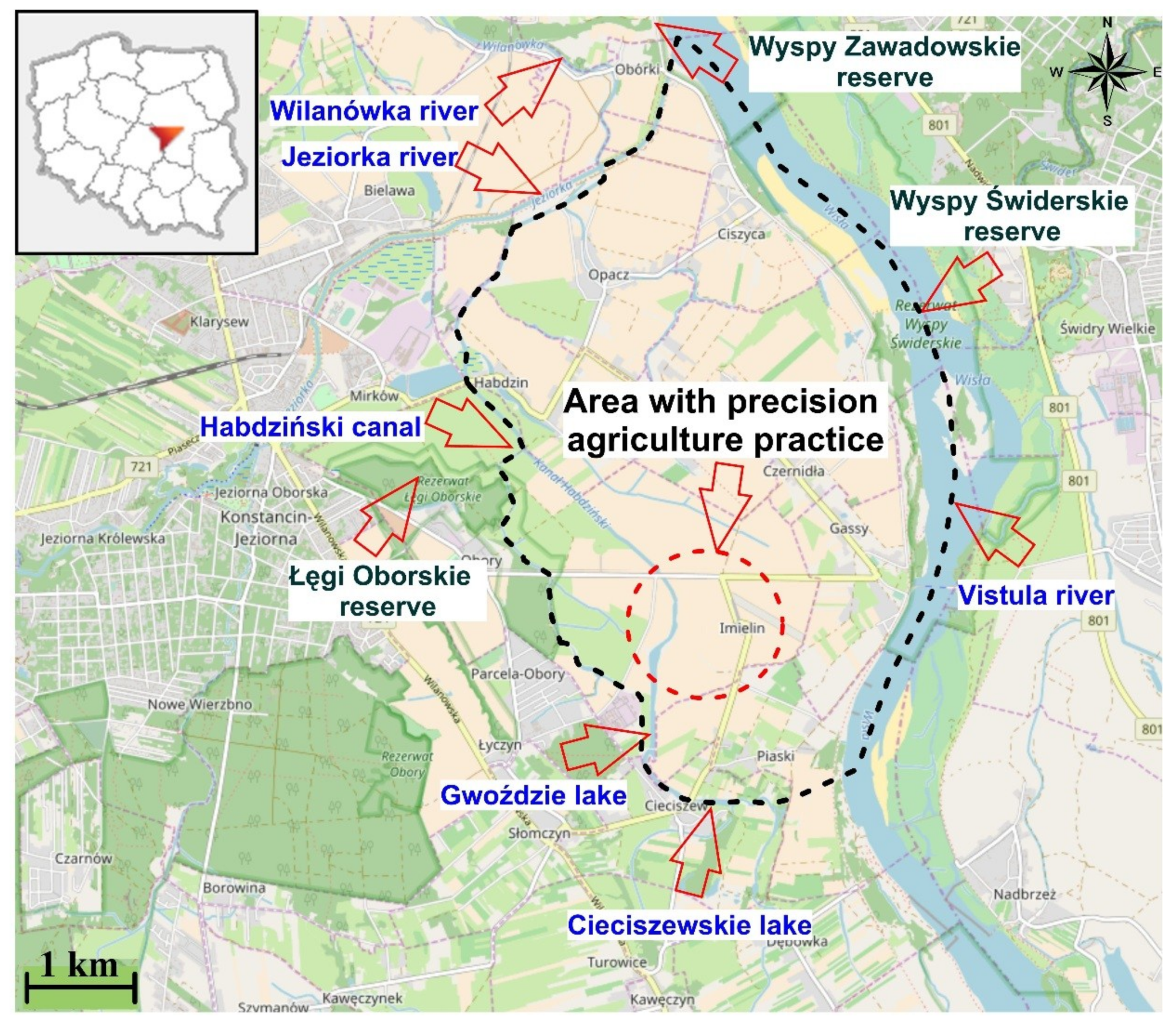
2.1. Study Area

The research area includes the contemporary floodplain of the Vistula River near Warsaw, Poland. The area covers ca. 17.5 km². From the north, east, and west, it is surrounded by nature reserves: Wyspy Zawadowskie, Wyspy Świderskie, and Łegi Oborskie (part of the Chojnowski Landscape Park), respectively (Figure 1).

The whole area is covered by a drainage system with numerous ditches and excavations. Noteworthy is a culvert, located in the northern part of the area, carrying the Wilanówka river waters under the artificial channel of the Jeziorka River.

On the south side, there are the Gwoździe Lake and Cieciszewskie Lake that mark the boundary of the modeled area. The west side of the modeling area borders on the Habdziński canal.

Falkowski et al. [46] reported that the basement of the contemporary alluvia observed in the research area forms a morphological protrusion composed of glaciotectonically disturbed and uplifted Neogene lacustrine clays and Pleistocene glacial deposits covered by a residual lag composed of glacial gravels and pebbles.

The floodplain, tapering to the south, is limited to the west by a Pleistocene glacial upland. From the east and north, the floodplain is limited by embankments of the Vistula and Jeziorka rivers. The area is relatively flat and falls towards the north following the course of the Vistula River.

In the southern part, agricultural areas of approximately 40 ha covered by the precision agriculture program are located. The cultivation of cereals, mainly wheat, is typical for this region. Agricultural fields lie approximately at 88 m above sea level (a.s.l). The altitudes within the modeled site are in the range of 86.39 m a.s.l. to 89.39 m a.s.l. Observed groundwater levels vary from 84.37 m a.s.l. to 86.62 m a.s.l. The average annual precipitation in the study area is around 550 mm. The annual average temperature for this site is 9 °C. Groundwater environment in the study area has a good chemical status compared with the groundwater quality standard presented in the Regulation of the Minister of the Environment of Poland [47].

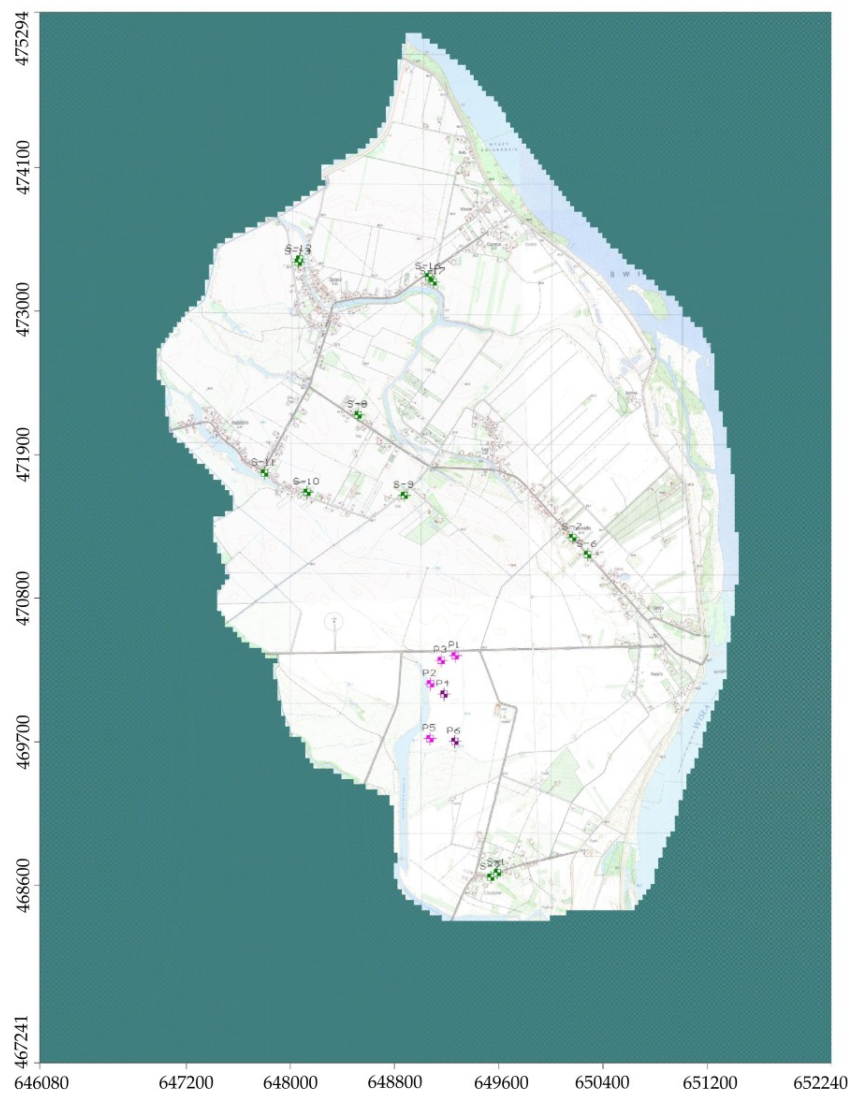
2.2. Field and Laboratory Studies

During the site inspections and field studies, soil samples were collected for further analysis of contaminant migration parameters, i.e., parameters of advection, dispersion, and sorption, respectively. In a group of advection parameters the following were measured: hydraulic conductivity, effective porosity, and flow velocity. The dispersion coefficient and longitudinal and transverse (horizontal and vertical) dispersivity were determined to specify the process of dispersion. For sorption, the retardation factor as well as distribution coefficient were assessed.

Six undisturbed soil samples were taken from the vicinity of piezometers located in agricultural fields using a stainless steel tube sampler (diameter 89 mm, length 600 m). Groundwater samples were collected in accordance with the procedure outlined in EN ISO 5667-3 [48] and ISO 5667-11 [49]. Before sampling, the top water in each piezometer was carefully pumped out using a submersible pump. The pump was rinsed with distilled water each time before the water sample was taken. To assure sampling appropriateness, each pumping was accompanied with simultaneous measurements of pH, temperature, and electrical conductivity. All samples were collected with great care taking into consideration that about 30% of the monitoring results may be biased due to inappropriate sampling and sample transportation [50]. As part of this study, an observation network of the level of groundwater and its quality was set up, including dug wells and observation piezometers (Figure 2). In total, the observation network consisted of twelve dug wells located within the research area and six piezometers in the fields with precision agriculture practice.

All of the observation points were leveled and connected to the National Geodetic Network. The depth to the groundwater table was measured using a hydrogeological whistle. Coordinates of dug wells (X, Y) were set according to “PUWG 1992” geodetic system using GPS-RTK equipment. In addition, water-level drops were marked out in surface watercourses within and on the boundaries of the analyzed area.

Physical properties of the soils were determined in accordance with the standards PN-EN ISO 14688-1:2006 [51], PN-B-02480:1986 [52], and PN-88/B-04481 [53], respectively. Physico-chemical properties of the soils and contaminant solutions (sodium chloride, ammonium nitrate), e.g., pH and EC were determined using a multimeter 18.52.01 (Eijkelkamp, Giesbeek, The Netherlands). Concentrations of selected pollutants were determined spectrophotometrically using a UV-VIS DR 6000 spectrophotometer (Hach Lange type, Düsseldorf, Germany).

In the next step, attention was paid to the identification of the parameters of migration of contaminants in the soil-water environment, in particular advection, dispersion, and sorption in dynamic conditions. The parameters responsible for migration, e.g., the hydraulic conductivity, flow velocity, porosity, dispersion coefficient, dispersivity, and retardation factor were determined using a Trautwein apparatus in the saturated conditions using the constant head method with regard to the ASTM D5084-00 procedure [54].

Hydraulic conductivity k was calculated using the following formula:

$$k=\frac{\mathsf{\Delta }V}{A·i·\mathsf{\Delta }t}$$

(2)

where ΔV—volume of the liquid, (m³); A—cross-section area of the soil sample, (m²); i—hydraulic gradient, (-); Δt—time, (s).

The experiment was based on the assumption that filtration of the liquid through the soil sample should last until the pore volume of flow is exchanged twice [55]. According to this assumption, the pore volume of flow (PVF) was treated as the sum of the flow in relation to the volume of soil pores opened for filtration. The PVF was calculated using the expression:

$$\mathrm{PVF}= \frac{k·i·\mathsf{\Delta }t}{n·L}$$

(3)

where n—total porosity of the soil sample, (-); L—length of the soil sample, (m).

The effective porosity n_e was calculated on the basis of performed column tests with reference to the formula presented by Marciniak et al. [56]:

$$n_e=\frac{q·t}{\pi ·L·r^2}$$

(4)

where q—flow rate (m³ s⁻¹); t—time required for exchange of one pore volume of flow, (s); r—radius of the soil sample, (m).

Before the test, the samples were soaked with distilled water until the flow stabilized, which was observed by the equality of the volumes of water flowing in and out of the sample. To imitate the stress conditions in the soils tested, a confining pressure was applied. Effluent samples were collected at different time intervals regarding the flow rate and the volume of solution that passed through the soil sample during the experiment. On this basis it was possible to control if any variations of the flow velocity occur.

After the flow stabilized, the injection of contaminants (sodium chloride, ammonium nitrate) was started from the bottom to the top of the sample. Chloride solution prepared based on sodium chloride was treated as a non-reactive marker, while nitrate solution prepared based on ammonium nitrate fertilizer was treated as a reactive one. During the experiment, the concentration, flow rate, and volume of solution that filtered through the sample in specific time intervals were measured. The concentrations of chloride and nitrate ions were measured with reference to the Mohr [57] and 8171 HACH methods [58], respectively.

Initial values of retardation factors R used as input data in further numerical studies were calculated based on the following formula [59]:

$$R=\frac{t_r}{t_o}$$

(5)

where t_r—time required to reach the maximum concentration of the reactive marker (nitrate), (s); t_o—time required to reach the maximum concentration of the non-reactive marker (chloride), (s).

Based on retardation factors R obtained from the column studies, it was possible to determine distribution coefficients K_d for each sample tested. The calculations were made using the transformed formula presented by Zhu and Anderson [60]:

$$R=1+\frac{{\rho }_d}{n_e}·K_d$$

(6)

where ρ_d—dry bulk density, (kg L⁻¹); K_d—partition coefficient, (L kg⁻¹).

Coefficients of hydrodynamic dispersion were calculated based on the following equations:

$$D_L= {\alpha }_L·v+D_M^{*}$$

(7)

$$D_T= {\alpha }_T·v+D_M^{*}$$

(8)

where D_L—longitudinal hydrodynamic dispersion coefficient, (m² s⁻¹); D_T—transverse hydrodynamic dispersion coefficient, (m² s⁻¹); $D_M^{*}$—effective diffusion coefficient, (m² s⁻¹); α_L—longitudinal dispersivity, (m); α_T—transverse dispersivity, (m); v—flow velocity, (m s⁻¹).

Longitudinal dispersivity was defined based on the formula presented by Appelo and Postma [61]:

$${\alpha }_L=0.1 x$$

(9)

where x—length of the filtration path, (m).

Horizontal transverse dispersivity (${\alpha }_{TH}$) and vertical transverse dispersivity (${\alpha }_{TV}$) were calculated using the following expressions [62,63]:

$${\alpha }_{TH}=0.1 {\alpha }_L$$

(10)

$${\alpha }_{TV}=0.01 {\alpha }_L$$

(11)

In this study, the half-life t_1/2 was used as a measure of nitrate decomposition in the denitrification process. First-order decay coefficient λ concerning denitrification was calculated in relation to half-life time t_1/2 of nitrates using the following equation [64]:

$$\lambda =\frac{0.693}{t_{1/2}}$$

(12)

A summary of the parameters used for numerical studies is presented in

Table 1. Hydrogeological parameters of model layers.

Layer	Hydraulic Conductivity k	Specific Yield a ${\mathit{S}}_{\mathit{y}}=0.117\sqrt[7]{\mathit{k}}$	Specific Storage b Ss	Total Porosity b n	Effective Porosity c ne
	(m day−1)	(-)	(m−1)	(-)	(-)
1	0.864	0.115	1.28 × 10−4	0.43	0.33
2	0.311	0.099	2.55 × 10−3	0.40	0.14
3	8.640	0.159	1.65 × 10−4	0.39	0.30
4	328.320	0.268	7.56 × 10−4	0.34	0.28
5	190.080	0.248	1.65 × 10−4	0.39	0.30
6	0.0016	0.047	1.92 × 10−3	0.40	0.04

Notes: a, b, c—according to: Bieciński [65], Batu [66] and Marciniak et al. [56], respectively.

.

The space of the conceptual model was set in a horizontal plane (XY) using a mesh with a side of 200 m. On this basis, longitudinal dispersivity was equal to 20 m. Horizontal transverse dispersivity and vertical transverse dispersivity were defined as 2.0 m and 0.2 m, respectively. Molecular diffusion $D_M^{*}$ for nitrates was adopted from Frind et al. [67] as 5 × 10⁻⁵ m² d⁻¹.

The half-life of nitrate degradation was adopted for modeling purposes based on literature research (

Table 2. Half-life of nitrates and calculated first order decay coefficients.

No.	Half-Life t1/2 (Years)	Reference	First-Order Decay Coefficient λ (Day−1)
1	1−2.3	[67]	8.25 × 10−4–1.90 × 10−3
2	20	[68]	9.49 × 10−5
3	1.4 *−7.5 **	[69]	2.53 × 10−4–1.36 × 10−3
4	3.7	[70]	5.13 × 10−4
5	3.7	[71]	5.13 × 10−4
6	1.2−2.1	[72]	9.04 × 10−4–1.58 × 10−3

Notes: * for the area where organic matter is present, ** for the area where organic matter is absent.

).

Eventually, the best calibration results were obtained for the first-order decay coefficient adopted at the level of λ = 5.13 × 10⁻⁴ day⁻¹.

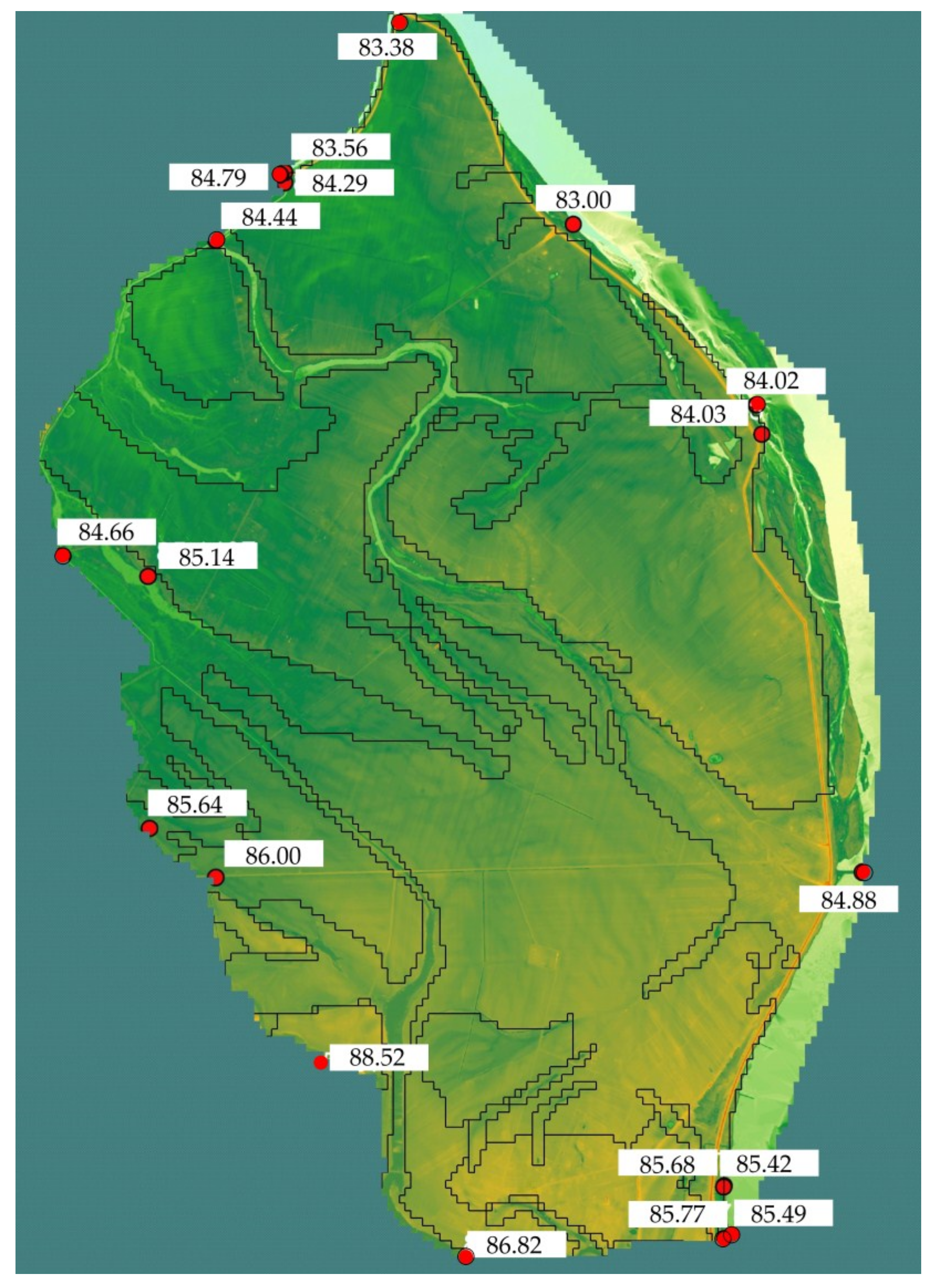
2.3. Numerical Modeling

To determine the parameters of the equation describing transport of contaminants in the soil-water environment, CXTFIT software was used [73]. The parameters were calculated based on the results of dynamic (column) investigations. The key of the procedure used in this methodological approach was the most accurate adjustment of the theoretical (modeled) curve to the curve obtained from experimental research, using numerical optimization methods [74]. The parameter estimation was carried out in accordance with the nonlinear optimization algorithm presented by Marquardt [75].

Owing to the fact that numerous literature studies [76,77,78,79,80] indicate that the CXTFIT package is very popular in estimating the migration parameters of pollutants, including non-reactive markers, pesticides, heavy metals, radionuclides as well as organic and inorganic compounds, the attempt was made in this study to check its utility for predicting parameters of migration of contaminants originating from agricultural fields.

Visual Modflow, considered an international standard for simulating and forecasting groundwater conditions and groundwater or surface-water interactions [30,81], was applied for numerical studies in presented study area. The MT3DMS, as a part of Visual Modflow software, was used to create a three-dimensional transport model that simulates 3D advective-dispersive transport of dissolved solutes (nitrates) in groundwater. As the result of numerical modeling, scenarios of the spread of pollutants in the groundwater environment with respect to the geological conditions were presented on isoline maps. Three-dimensional transport of contaminants was described using the equation presented by Zheng and Wang [82]:

$$\frac{\partial C}{\partial t}=\frac{\partial }{\partial x_i}\left[D_{ij}\frac{\partial C}{\partial x_j}\right]-\frac{\partial }{\partial x_i}\left(v_{i}C\right)+\frac{q_s}{n}{C}_s+\sum R_n$$

(13)

where C—contaminant concentration, (mg L⁻¹); t—time, (s); x_i—distance along the respective Cartesian coordinate axis, (m); D_ij—hydrodynamic dispersion coefficient tensor, (m² s⁻¹); v_i—pore water velocity, (m s⁻¹); q_s—volumetric flow rate per unit volume of aquifer, (m³ s⁻¹); C_s—concentration of the source or sink flux for contaminant, (mg L⁻¹); n—porosity of the porous medium, (-); R_n—chemical reaction term representing retardation factor, (-).

A significant step in numerical modeling of groundwater flow and migration of the contaminant plume in the soil-water environment was the preparation of a conceptual model (Figure 3).

Generally, the model represented the authors’ interpretation of available hydrogeological data, based on data from field tests, and laboratory and literature studies. Then, the conceptual model was translated into a numerical model by setting its boundary and initial conditions, and hydrogeological parameters. The final step of the numerical modeling studies was the model validation and calibration.

The model body was constructed as the effect of the dissection of the dynamics of geomorphological processes during the bankfull flow, identified using the remote sensing tools, which was confirmed by data obtained from drill holes. Subsequently, the created model was used as the initial stage for developing the transient model, taking into account the time-dependent changes, resulting from the variability of recharge (infiltration) conditions. Then, using the MT3DMS tool, an attempt was made to simulate the migration of nitrates from the experimental field where the precision agriculture techniques were applied. The basic stage of the research was to simulate the response of the groundwater system to the change of external conditions.

The morphology of the research area was precisely identified with the use of satellite images and elevation data obtained from the airborn laser scanning (ALS) within the ISOK project (IT System of the Country’s Protection against Extreme Hazards). The validity of using aerial photographs, and LIDAR data in determining geomorphological features were presented by Wierzbicki et al. [83].

The obtained data was stored in the GIS spatial database created for the purpose of this study. It allowed a series of thematic layers to be created that, in the next step of this research, became a basis for creating a numerical model of groundwater dynamics and contaminant mass transport. The concept of the modeled system assumed subdivision of the block of numerical model into six layers separated based on the values of the filtration parameters. The data concerning the morphology of the first layer, corresponding to the superficial deposits, was taken from the resources of the Geodetic and Cartographic Documentation Centre in the form of Digital Elevation Model (DEM). The remaining layers, with exception of the sublayer, were mapped using the flat layers with an average thickness of river sediments in a given study area. The morphology of the sublayer, which is also an impermeable boundary of the model, was interpolated based on the information from the cards of deep boreholes, collected by the Central Geological Archive of the Polish Geological Institute—National Research Institute.

Defining the concept of the aquifer system and then separating it from the surroundings in the form of a three-dimensional model allows for calculations of groundwater flow and contaminant transport using iterative methods.

While extracting the modeled system from the surroundings, it was assumed that groundwater of the floodplain area saturates the uniform alluvial reservoir. The reservoir is confined on three sides by surface watercourses that are in hydraulic connection with groundwater. Due to the clogging, this connection is limited largely in the area of oxbows located in the west side of the modeled area.

For setting the model boundaries, three types of conditions were applied: 1st type—Ditichlet’s, 2nd type—Neumann’s, and 3rd—Cauchy’s conditions, respectively.

The eastern, northern, and western boundaries of the system were modeled using the third type of boundary condition—the RIVER variant. By using this type of condition the influence of surface water on the groundwater flow was simulated. The RIVER package reflected the interaction between the surface water and groundwater through a seepage layer separating the surface water body from the groundwater system.

The southern boundary was modeled using the first type condition—the CONSTANT HEAD variant—based on the measurements of groundwater level in landlocked depressions. The CONSTANT HEAD was used in the form of an external boundary condition assigned by setting values of hydraulic heads to the boundary surface of a separated model system.

Neumann’s boundary condition was set using the RECHARGE variant of the Visual Modflow software. This variant was used to simulate recharge to the groundwater system as a result of percolating precipitation into a deeper part of the soil profile.

Infiltration rate was determined with reference to the lithology described by Pazdro and Kozerski [84]. Concerning the infiltration rate equal to 0.20 and precipitation equal to 550 mm year⁻¹, the infiltration was defined as 110 mm year⁻¹ for the study area.

To assess the threat of groundwater contamination caused by nitrates, the formula presented by Duda et al. [85] was used:

$$C_{{\mathrm{NO}}_3}=\frac{L_N}{I_e}·443$$

(14)

where $C_{{\mathrm{NO}}_3}$—contamination recharge to groundwater, (mg L⁻¹); L_N—nitrogen load leached from soil profile, (kg N ha⁻¹ year⁻¹); I_e—effective infiltration, (mm year⁻¹), 443—factor of unit conversion, (-).

Nitrogen load leached from the soil profile was calculated using the formula [85]:

$$L_N=0.15· D_N$$

(15)

where 0.15—coefficient determining which part of fertilizer was leached to groundwater in an agricultural area [86]; D_N—nitrogen dose in fertilizer applied, (kg N ha⁻¹ year⁻¹).

The principal stage of modeling was the design and calibration of the filtration dynamics model. The main goal of model calibration was to obtain the highest consistency between the hydrodynamic state of the groundwater stream recorded during fieldwork and the state obtained as a result of computer simulation. The error analysis was performed to assess the conformity of the calculated values of hydraulic heads with the values estimated during fieldwork. Model verification was carried out on the basis of checking the following types of errors: residual mean error, absolute residual mean error, root mean square error, and normalized root mean square error. A similar approach of model verification was presented by Bujakowski et al. [87].

3. Results and Discussion

3.1. Numerical Studies

It was revealed that the modeling surface varied with numerous footprints of overbank flows (Figure 4).

An innovative element of the presented research is the consideration of the effect of the dynamics of geomorphological processes in the overbank zone on the groundwater flow conditions. The results of the numerical modeling studies have shown that a particular impact on the groundwater dynamics and, consequently, transport phenomena, is exerted by the geomorphological forms that generally can be subdivided into the zone of transformed floodplain, crevasse splays, and crevasses (Figure 5).

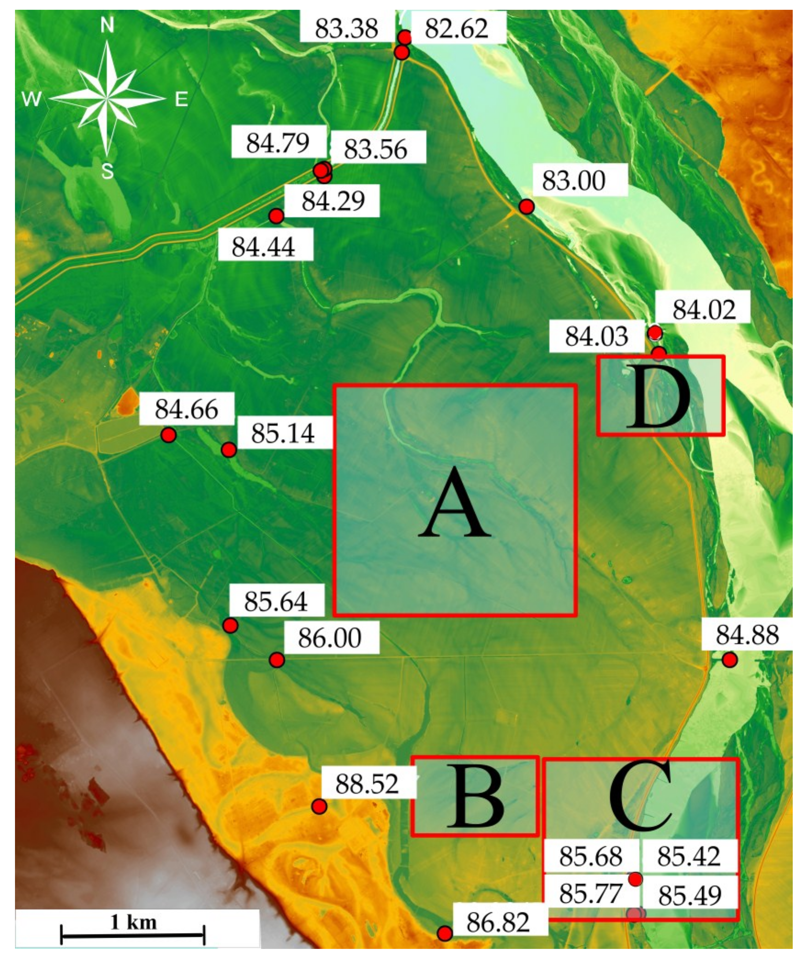
3.1.1. Zone of the Transformed Floodplain

It was observed that the packet of low-permeable alluvial soils of Atlantic age has been partially or completely removed from the proximal zone of the floodplain. The alluvial soils represented by loams and clays, and characterized by low hydraulic conductivity, initially had an isolating function. The nature of their sedimentation caused the overlying deposits to be compact and they extended over the whole floodplain area, separating the subsurface water level from the deeper one. Rosenberry and Healy [88] reported that even a thin layer of alluvial deposits has an impact on seepage between the river and groundwater. Due to the erosive activity of the bankfull discharge, which is caused, inter alia, by ‘wilding of the rivers’, the cover of alluvial soils was removed in many places of the modeled area, creating hydrogeological windows connecting the shallow and the deeper groundwater levels and ensuring free water exchange between them. In such conditions, the contaminants from the shallow level can easily migrate to the deeper part of the specific zones which can be seen in Figure 6.

Additionally, this research revealed that the zone of the transformed floodplain, where the Atlantic alluvial soils were eroded, constitute drainage collectors, which are penetrated by contaminants after some time. Figure 7 presents the scenarios of nitrate migration in the study area one year after the fertilizer application considering the differentiated rates of precipitation applied in the model.

Under average conditions of precipitation for a given area, effective infiltration is 110 mm year⁻¹. In such a situation, the majority of the studied area is drained by the Vistula River. For the observed oxbows, landforms of overbank flows, and artificial ditches the flow rate is insignificant. Groundwater levels fall towards the north-east and form below the bottom of these landforms. In such conditions, the zone of the transformed floodplain has only an impact on infiltration rate, with no effect on groundwater levels. This tendency is observed mainly in a period of a low and an average precipitation (Figure 7a). Deviations from this tendency are observed during the occurrence of several days with intense rainfall. At that time, the study area is fully saturated with water. The zone of transformed floodplain, both those constituting a combined system of surface watercourses as well as those masked in the landscape due to secondary filling with sediments, become zones of intense drainage (Figure 7b). In practice, related to environmental engineering and environmental protection, this may be a valuable premise in designing the monitoring system of the dynamics and groundwater quality coming from infiltration in agricultural areas.

Since in our study the priority was given to saturated zone modeling, the authors only focused on conditions of full saturation of the porous medium. However, in order to perform the comprehensive analysis of nitrogen transport in the soil-water environment (unsaturated and saturated zone), a broader scope of data and accompanying processes should be taken into consideration. For example, the mechanistic models, i.e., TOUGHREACT-N would be worth considering [89]. An investigation of temporal and biochemical changes of nitrogen as well as interactions between physical, biochemical, hydrological, and geological features controlling transport of considered pollutant would aid in proper interpretation of its fate. The study presented by Dwivedi et al. [90] is a comprehensive example of integrating geophysical data, mineralogical analyses, monitoring of water levels, and water quality in the interpretation of the impact of several involved issues on nitrogen behavior. In the quoted study, 3-D simulations performed using the PFLOTRAN model were used in mapping spatial and temporal changes related to nitrogen fluxes. Identification of nitrogen “hot moments” using the mentioned model is crucial in analyses dealing with the study of nitrogen fate and transport, and the mitigation of risk associated with its occurrence in the soil-water environment. Similarly, Dwivedi and Mohanty [91] paid attention to the need of analysis of the interaction between several factors, i.e., precipitation, composition of the vadose zone and its heterogeneity influencing the long-term behavior of nitrate in the soil-water environment. The quoted authors used the entropy concept and Hurst exponent for analyses of the spatial and temporal changes of nitrate in groundwater. Their study highlighted the fact that precipitation has a significant impact on the extent of nitrate leaching from agriculture. Dwivedi and Mohanty [91] also demonstrated that the agricultural areas are more prone to nitrate contamination due to fertilization and unconfined aquifers are more susceptible to pollution compared to confined ones. Arora et al. [92] presented the use of continuum-scale models, i.e., dual-porosity, dual-permeability, multiple porosity, and mobile-immobile models, for simulating preferential flow of contaminants. The mentioned authors pointed out that farming practice in agricultural areas can significantly modify soil structure and the density of its macropore. As a result, differences in macropore density contribute to increased contaminant leaching as preferential flow can occur through macropores. The approach proposed by Arora et al. [92] can be applied to quantify contaminant migration in agricultural lands.

3.1.2. Crevasse Splays and Crevasses

Crevasse splays are forms of intense sedimentation in the presence of overbank flow. According to Kargel et al. [93], crevasse splays are defined as sheetflood deposits formed by subsidiary river channels as a result of point failure of a levee. They are most often located at the outlet of erosional cuts in the distal part of the floodplain. The material accumulated in this zone contributes to the increase of the thickness of sandy deposits composing the subsurface aquifer, increasing their conductivity and effective infiltration as well as affecting the inertia of the groundwater stream. Falkowska and Falkowski [5] showed that these landforms consist of two main sedimentological types of surface. It was observed in zones of elongated ridges that a layer of cohesive deposits (loams, silty loams, and silty clays) overlies a sand layer with silt intercalations. Between the ridges, the near-surface layer is composed of silty loams and silty clays, locally intercalated with sands of various grain size, up to 30 cm in thickness. As has been found out, crevasse splays are zones of intensified effective infiltration.

Crevasses can be defined as narrow channels created by erosion processes. They are formed when the water stream surpasses the bankfull stage of natural embankments or when the embankment failure takes place. These landforms are characterized by a significant depth of up to several meters. The nature of the deposition during the falling of the flood causes these forms to be filled with low-density material. Falkowska and Falkowski [5] reported that two types of sediment profile dominate in this case: deposits (1) composed of fine and coarse sands, and (2) represented by silty sands. Crevasses are the drainage collectors during low-flow periods and the suppliers during the overbank stage. The velocity of filtration observed in these forms is 10 times higher than in the zone of the untransformed floodplain. The crevasses constitute intense drainage zones, creating preferential paths for migration of contaminants to the riverbed area. As reported by Bujakowski and Falkowski [11], these forms can also contribute to intensified filtration during low and high water stages, and consequently, to the safety of hydro-engineering structures. The quoted authors claimed that zones of preferential water flow can be effectively identified using morphogenetic analysis based on aerial and satellite images.

The crevasse splays and crevasses in the study area can be recognized with high accuracy in Figure 8.

3.2. Model Calibration

The calibration of hydraulic head was performed on the basis of groundwater level measurements in dug wells located within the modeled site. For nitrates, the piezometers located within the field with precision agriculture practice were taken into consideration. The numerical model of groundwater flow dynamics and nitrate transport was verified by checking several types of errors. For hydraulic heads, regarding normal precipitation (infiltration rate equal to 110 mm), the following errors were calculated: residual mean error of −0.033 m, absolute residual mean error of 0.169 m, root mean square error of 0.184 m, and normalized root mean square error (normalized RMS) of 7.786%. The observed versus calculated hydraulic heads for a case with an average precipitation of 550 mm (infiltration rate equal to 110 mm year⁻¹) are presented in Figure 9.

In case of intense rainfall (infiltration rate equal to 300 mm year⁻¹) the following errors were obtained: residual mean error of −0.331 m, absolute residual error of 0.331 m, root mean square error of 0.354 m, and normalized root mean square error of 14.988%. The increased value of normalized RMS obtained for this case is a result of artificially simulated intense precipitation while taking into account real values of groundwater levels measured during field investigations.

The summary of nitrate concentrations observed and calculated in the model is presented in

Table 3. Observed and calculated nitrate concentrations.

Concentration		Piezometer
		1	2	3	4	5	6
Observed	mg L−1	0.90	0.30	0.10	0.20	0.20	0.20
Calculated	mg L−1	0.36	0.21	0.38	0.34	0.21	0.25

.

Additionally, in the case of nitrate modeling, the following errors were calculated: residual mean error of −0.023 mg L⁻¹, absolute residual mean error of 0.188 mg L⁻¹, root mean square error of 0.261 mg L⁻¹, and normalized root mean square error of 32.609%.

4. Conclusions

The availability of precise geo-environmental data allows for more and more accurate mapping of the natural environment using numerical modeling techniques. Precise remote sensing tools (e.g., high-resolution images, multispectral satellite images, Light Detection and Ranging—LIDAR), conducted in the world since the 1930s, support the process of identification and valorization of the geological landforms that are seemingly masked in the surrounding landscape and therefore are difficult to recognize using conventional methods.

As shown in this study, the specific forms that can be characterized by highly sophisticated methods may be the key element in the description of the hydrogeological environment of the floodplain. Particularly important for the conditions of migration of contaminants, is the presence of secondary-filled erosional forms constituting drainage collectors in the area of the lowland river floodplain. Moreover, noteworthy is the increased infiltration rate of the water in these zones. Special attention should be paid to the proper recognition of geomorphological forms that can significantly affect the groundwater dynamics, and subsequently, the contaminant transport. On this basis, there is a real possibility to mark zones that could be particularly exposed to increased concentration of pollutants during heavy rainfall periods.

This study revealed that use of remote sensing data can be an effective tool allowing for separation of soil layers with diverse filtration parameters. Considering the occurrence of such layers in the model body had a significant impact on the model calibration results. The effect of this methodological approach has also been confirmed by Ćwiklińska et al. [15] and Bujakowski and Falkowski [94].

As presented by Falkowski [2] and Karabon [95], the arrangement of landforms occurring on the surface of the floodplain terrace can be combined with the presence of specific geological structures in the basement of the modern alluvium deposits. The enormous progress in remote sensing studies was, in addition to the multispectral imaging, the use of airborne laser scanning technology that allows for identification of microrelief features.

The use of numerical modeling techniques, combined with the results of laboratory studies, contributed to a comprehensive overview on predicting the contaminant migration in the soil-water environment. The presented approach of the geological research methodology adopted for the agricultural area of the Polish Lowlands provided valuable information about the possible susceptibility to water pollution in some parts of the modeling area, primarily in the zone of the transformed floodplain.

The proposed tools and methods have contributed to a significant increase in the accuracy of the description of the environment in the research area. The development of remote sensing techniques, in particular using ALS laser scanning data, and high-resolution, multi-spectral satellite image in combination with numerical modeling, enabled hydrogeological analysis to be carried out with a great precision.

According to the aforementioned reflections, such methods should be adopted as the basic step of the procedure used in recognizing other areas susceptible to pollution.

Fulfilling the idea of a sustainable development of agricultural areas and knowledge-based management, the results of such analyses may influence the efficiency of management in farming practice in the agriculturally rich valley of the Vistula River.

References

1. Pierce, A.R.; King, L.S. Spatial dynamics of overbank sedimentation in floodplain systems. Geomorphology 2008, 100, 256–268. [Google Scholar] [CrossRef]
2. Falkowski, E. Historia i prognoza rozwoju układu koryta wybranych odcinków rzek nizinnych Polski. Biul. Geol. 1971, 12, 5–121. (In Polish) [Google Scholar]
3. Fryirs, K.A.; Brierley, G.J. Geomorphic Analysis of River Systems: An Approach to Reading the Landscape; John Wiley & Sons, Ltd.: Chichester, UK, 2013; pp. 1–8. [Google Scholar]
4. Kamykowska, M.; Kaszowski, L.; Krzemień, K. Kartowanie koryt rzecznych. In Struktura Koryt Rzek i Potoków (Studium Metodyczne); Krzemień, K., Ed.; Instytut Geografii i Gospodarki Przestrzennej UJ: Kraków, Poland, 2012; pp. 15–42. ISBN 978-83-88424-82-3. (In Polish) [Google Scholar]
5. Falkowska, E.; Falkowski, T. Trace metals distribution pattern in floodplain sediments of a lowland river in relation to contemporary valley bottom morphodynamics. Earth Surf. Process. Landf. 2015, 40, 876–887. [Google Scholar] [CrossRef]
6. Masiello, C.A.; Gallagher, M.E.; Randerson, J.T.; Deco, R.M.; Chadwick, O.A. Evaluating two experimental approaches for measuring ecosystem carbon oxidation state and oxidative ratio. J. Geophys. Res. 2008, 113, G03010. [Google Scholar] [CrossRef]
7. Dhivert, E.; Grosbois, C.; Rodrigues, S.; Desmet, M. Influence of fluvial environments on sediment archiving processes and temporal pollutant dynamics (Upper Loire River, France). Sci. Total Environ. 2015, 505, 121–136. [Google Scholar] [CrossRef] [PubMed]
8. Dwivedi, D.; Riley, W.J.; Torn, M.S.; Spycher, N.; Maggi, F.; Tang, J.Y. Mineral properties, microbes, transport, and plant-input profiles control vertical distribution and age of soil carbon stocks. Soil Biol. Biochem. 2017, 107, 244–259. [Google Scholar] [CrossRef]
9. Falkowski, T. The application of geomorphological analysis of the Vistula River, Poland in the evaluation of the safety of regulation structures. Acta Geol. Pol. 2007, 57, 377–389. [Google Scholar]
10. Falkowski, T. The importance of recognition of polygeny for the rational utilisation of river valleys in Polish Lowland. In Proceedings of the International Symposium Engineering Geology and the Environment, Athens, Greece; A.A. Balkema: Rotterdam, The Netherland, 1997; pp. 107–111. [Google Scholar]
11. Falkowski, T. Alluvial bottom geology inferred as a factor controlling channel flow along the Middle Vistula River, Poland. Geol. Q. 2007, 51, 91–101. [Google Scholar]
12. Bujakowski, F.; Falkowski, T. Wykorzystanie lotniczego skaningu laserowego do oceny warunków przepływu wód w osadach równi zalewowej. Prz. Geol. 2017, 65, 443–449. (In Polish) [Google Scholar]
13. Li, J.; Bristow, C.S. Crevasse splay morphodynamics in a dryland river terminus: Río Colorado in Salar de Uyuni Bolivia. Quat. Int. 2015, 377, 71–82. [Google Scholar] [CrossRef]
14. Yuill, B.T.; Khadka, A.K.; Pereira, J.; Allison, M.A.; Meselhe, E.A. Morphodynamics of the erosional phase of crevasse-splay evolution and implications for river sediment diversion function. Geomorphology 2016, 259, 12–29. [Google Scholar] [CrossRef]
15. Ćwiklińska, M.; Kuźniar, P. Influence of Earlier forms of the Bed of the Middle Vistula River on the Course of Centemporary Floods. In Proceedings of the International Conference Towards Natural Flood Reduction Strategies, Warsaw, Poland, 6–13 September 2003. [Google Scholar]
16. Goldschneider, A.A.; Haralampides, K.A.; MacQuarrie, K.T. River sediment and flow characteristics near a bank filtration water supply: Implications for riverbed clogging. J. Hydrol. 2007, 344, 55–69. [Google Scholar] [CrossRef]
17. Bowles, C.J.; Cowgill, E. Discovering marine terraces using airborne LiDAR along the Mendocino-Sonoma coast, northern California. Geosphere 2012, 8, 386–402. [Google Scholar] [CrossRef]
18. Merritts, D.; Bull, W.B. Interpreting Quaternary uplift rates at the Mendocino triple junction, northern California, from uplifted marine terraces. Geology 1989, 17, 1020–1024. [Google Scholar] [CrossRef]
19. Regard, V.; Pedoja, K.; De La Torre, I.; Saillard, M.; Cortés-Aranda, J.; Nexer, M. Geometrical Trends within Sequences of Pleistocene Marine Terraces: Selected Examples from California, Peru, Chile and New-Zealand. 2017. Available online: https://hal.archives-ouvertes.fr/hal-01497422 (accessed on 24 March 2018).
20. Alexandrowicz, S.W.; Klimek, K.; Kowalkowski, A.; Mamakowa, K.; Niedziałkowska, E.; Pazdur, M.; Starkel, L. The evolution of the Wisłoka valley near Dębica during the Late Glacial and Holocene. Folia Quat. 1981, 53, 1–91. [Google Scholar]
21. Ward, J.V.; Malard, F.; Tockner, K.; Uehlinger, U. Influence of ground water on surface water conditions in a glacial flood plain of the Swiss Alps. Hydrol. Process. 1999, 13, 277–293. [Google Scholar] [CrossRef]
22. Bongiovanni, R.; Lowenberg-Deboer, J. Precision Agriculture and Sustainability. Precis. Agric. 2004, 5, 359–387. [Google Scholar] [CrossRef]
23. Baum, R.; Wojszczuk, K.; Wawrzynowicz, J. Miejsce i rola rolnictwa precyzyjnego w koncepcji zrównoważonego rozwoju gospodarstw rolnych. Ekon. i Środowisko 2012, 1, 71–83. (In Polish) [Google Scholar]
24. Kim, H.-S.; Park, S.-R. Hydrogeochemical characteristics of groundwater highly polluted with nitrate in an agricultural area of Hongseong, Korea. Water 2016, 8, 345. [Google Scholar] [CrossRef]
25. Gworek, B.; Dmuchowski, W.; Koda, E.; Marecka, M.; Baczewska, A.H.; Brągoszewska, P.; Sieczka, A.; Osiński, P. Impact of the Municipal SolidWaste Łubna Landfill on Environmental Pollution by Heavy Metals. Water 2016, 8, 470. [Google Scholar] [CrossRef]
26. Koda, E.; Osiński, P.; Sieczka, A.; Wychowaniak, D. Areal Distribution of Ammonium Contamination of Soil-Water Environment in the Vicinity of Old Municipal Landfill Site with Vertical Barrier. Water 2015, 7, 2656–2672. [Google Scholar] [CrossRef]
27. Caruso, A.; Ridolfi, L.; Boano, F. Impact of watershed topography on hyporheic exchange. Adv. Water Res. 2016, 94, 400–411. [Google Scholar] [CrossRef]
28. Dwivedi, D.; Steefel, C.I.; Arora, B.; Bisht, G. Impact of intra-meander hyporheic flow on nitrogen cycling. Procedia Earth Planet. Sci. 2017, 17, 404–407. [Google Scholar] [CrossRef]
29. Gruszczyński, T.; Małecki, J. Numerical model of transient filtration for the part of the Vistula valley in the mouth of the Świder river. Geologos 2006, 10, 65–74. (In Polish) [Google Scholar]
30. Yang, Q.; Lu, W.; Fang, Y. Numerical modeling of three dimension groundwater flow in Tongliao (China). Procedia Eng. 2011, 24, 638–642. [Google Scholar] [CrossRef]
31. Lima, M.L.; Romanelli, A.; Massone, H.E. Assessing groundwater pollution hazard changes under different socio-economic and environmental scenarios in an agricultural watershed. Sci. Total Environ. 2015, 530–531, 333–346. [Google Scholar] [CrossRef] [PubMed]
32. Ghoraba, S.M.; Zyedan, B.A.; Rashwan, I.M.H. Solute transport modeling of the groundwater for quaternary aquifer quality management in Middle Delta, Egypt. Alex. Eng. J. 2013, 52, 197–207. [Google Scholar] [CrossRef]
33. Verruijt, A.; Koda, E. Analysis of Pollution Control by Finite Elements. In Water Science and Technology Library; Computational Methods in Water Resources X, Vols 1 And 2; Peters, A., Wittum, G.P., Herrling, B., Meissner, U., Brebbia, C.A., Gray, W.G., Pinder, G.F., Eds.; Kluwer Academic Publisher: Heidelberg, Germany, 1994; Volume 12, pp. 1489–1495. [Google Scholar]
34. Koda, E.; Wienclaw, E. Flow and transport modelling in old landfill subsoil with vertical barrier. In Proceedings of the 16th International Conference on Soil Mechanics and Geotechnical Engineering, Vols 1–5: Geotechnology in Harmony with the Global Environment, Osaka, Japan, 12–16 September 2005; pp. 921–924. [Google Scholar]
35. Koda, E. Influence of vertical barrier surrounding old sanitary landfill on eliminating transport of pollutants on the basis of numerical modelling and monitoring results. Pol. J. Environ. Stud. 2012, 21, 929–935. [Google Scholar]
36. Koda, E.; Osinski, P.; Kolanka, T. Flow numerical modeling for efficiency assessment of vertical barriers in landfills. In Coupled Phenomena in Environmental Geotechnics: From Theoretical and Experimental Research to Practical Applications, Proceedings of International Symposium TC215 ISSMGE, Torino, Italy, 1–3 July 2013; Manassero, M., Dominijanni, A., Foti, S., Musso, G., Eds.; CRC Press: London, UK, 2013; pp. 693–698. [Google Scholar]
37. Szczepański, A. Prognozowanie Wydajności i Warunków Eksploatacji wód Podziemnych Metodą Analogii Hydraulicznych; Prace Geologiczne, nr 81; Wydawnictwa Geologiczne: Warszawa, Poland, 1974. (In Polish) [Google Scholar]
38. Małecki, J.J.; Nawalany, M.; Witczak, S.; Gruszczyński, T. Wyznaczanie Parametrów Migracji Zanieczyszczeń w Ośrodku Porowatym Dla Potrzeb Badań Hydrogeologicznych i Ochrony Środowiska. Poradnik Metodyczny; Uniwersytet Warszawski, Wydział Geologii: Warszawa, Poland, 2006. (In Polish) [Google Scholar]
39. Bradbury, K.R.; Gotkowitz, M.B.; Hart, D.J.; Eaton, T.T.; Cherry, J.A.; Parker, B.L.; Borchardt, M.A. Contaminant Transport Through Aquitards: Technical Guidance for Aquitard Assessment; Awwa Research Foundation: Denver, CO, USA, 2006. [Google Scholar]
40. Dąbrowski, S.; Kapuściński, J.; Nowicki, K.; Przybyłek, J.; Szczepański, A. Metodyka Modelowania Matematycznego w Badaniach i Obliczeniach Hydrogeologicznych—Poradnik Metodyczny; Ministerstwo Środowiska: Poznań, Poland, 2010. (In Polish) [Google Scholar]
41. Sabino, C.V.S.; Moreira, R.M.; Lula, Z.L.; Chausson, Y.; Magalhães, W.F.; Vianna, M.N. Contaminant transport in aquifers: “Improving the determination of model parameters”. In Application of Isotope Techniques to Investigate Groundwater Pollution; IAEA-TECDOC-1046; International Atomic Energy Agency: Vienna, Austria, 1998. [Google Scholar]
42. Sieczka, A.; Koda, E. Kinetic and equilibrium studies of sorption of ammonium in the soil-water environment in agricultural areas of Central Poland. Appl. Sci. 2016, 6, 269. [Google Scholar] [CrossRef]
43. Sieczka, A.; Koda, E. Identification of Nitrogen Compounds Sorption Parameters in the Soil-Water Environment of a Column Experiment. Ochr. Srodowiska 2016, 38, 29–34. (In Polish) [Google Scholar]
44. Fronczyk, J.; Sieczka, A.; Lech, M.; Radziemska, M.; Lechowicz, Z. Transport of nitrogen compounds through subsoils in agricultural areas: Column tests. Pol. J. Environ. Stud. 2016, 25, 1505–1514. [Google Scholar] [CrossRef]
45. Sieczka, A.; Koda, E. Evaluation of chlorides transport parameters in natural soils based on laboratory studies. In MendelNet 2017, Proceedings of 24th International PhD Students Conference; Cerkal, R., Brezinová Belcredi, N., Prokešová, L., Vacek, P., Eds.; Mendel University in Brno, Faculty of AgriSciences: Brno, Czech Republic, 2017; Volume 24, pp. 921–926. ISBN 978-80-7509-529-9. [Google Scholar]
46. Falkowski, T.; Ostrowski, P.; Siwicki, P.; Brach, M. Channel morphology changes and their relationship to valley bottom geology and human interventions; a case study from the Vistula Valley in Warsaw, Poland. Geomorphology 2017, 297, 100–111. [Google Scholar] [CrossRef]
47. Regulation of the Minister of Environment Dated 21 December 2015 on the Criteria and Method of Evaluating the Underground Water Condition (Journal of Laws 2016, Item 85). Available online: http://prawo.sejm.gov.pl/isap.nsf/DocDetails.xsp?id=WDU20160000085 (accessed on 23 March 2018).
48. PN-EN ISO 5667-3:2013-05. Jakość Wody—Pobieranie Próbek—Część 3: Utrwalanie i Postępowanie z Próbkami Wody; Polski Komitet Normalizacyjny: Warszawa, Poland, 2013. (In Polish) [Google Scholar]
49. PN-ISO 5667-11:2004. Jakość Wody—Pobieranie Próbek—Część 11: Wytyczne Dotyczące Pobierania Próbek Wód Podziemnych; Polski Komitet Normalizacyjny: Warszawa, Poland, 2004. (In Polish) [Google Scholar]
50. Nielsen, D.M. Practical Handbook of Environmental Site Characterization and Ground-Water Monitoring, 2nd ed.; CRC Press: Boca Raton, FL, USA, 2005. [Google Scholar]
51. PN-EN ISO 14688-1:2006. Badania Geotechniczne—Oznaczanie i Klasyfikowanie Gruntów—Część 1: Oznaczanie i opis; Polski Komitet Normalizacyjny: Warszawa, Poland, 2006. (In Polish) [Google Scholar]
52. PN-B-02480:1986. Grunty Budowlane—Określenia, Symbole, Podział i opis Gruntów; Polski Komitet Normalizacyjny: Warszawa, Poland, 1986. (In Polish) [Google Scholar]
53. PN-88/B-04481. Grunty Budowlane—Badania Próbek Gruntu; Polski Komitet Normalizacyjny: Warszawa, Poland, 1988. (In Polish) [Google Scholar]
54. ASTM D5084-00. Standard Test Methods for Measurement of Hydraulic Conductivity of Saturated Porous Materials Using a Flexible Wall Permeameter; ASTM International: West Conshohocken, PA, USA, 2001. [Google Scholar]
55. Bowders, J.; Daniel, D.E. Hydraulic conductivity of compacted clay to dilute organic compounds. ASCE J. Geotech. Eng. 1987, 113, 1432–1448. [Google Scholar] [CrossRef]
56. Marciniak, M.; Małoszewski, P.; Okońska, M. Wpływ efektu skali eksperymentu kolumnowego na identyfikację parametrów migracji znaczników metodą rozwiązań analitycznych i modelowania numerycznego. Geologos 2006, 10, 167–187. [Google Scholar]
57. PN-ISO 9297: 1994. Jakość Wody—Oznaczanie Chlorków—Metoda Miareczkowania Azotanem Srebra w Obecności Chromianu Jako Wskaźnika (Metoda Mohra); Polski Komitet Normalizacyjny: Warszawa, Poland, 1994. (In Polish) [Google Scholar]
58. Water Analysis Handbook, 7th ed.; Nitrate Cadmium Reduction Method 8171; Hach Company: Loveland, CO, USA, 2012.
59. Macioszczyk, A. (Ed.) Podstawy Hydrogeologii Stosowanej; Wydawnictwo Naukowe PWN: Warszawa, Poland, 2006. (In Polish) [Google Scholar]
60. Zhu, C.; Anderson, G. Environmental Applications of Geochemical Modeling; Cambridge University Press: Cambridge, UK, 2002. [Google Scholar]
61. Appelo, C.A.J.; Postma, D. Geochemistry, Groundwater and Pollution; A.A. Balkema: Rotterdam, The Netherlands, 1999. [Google Scholar]
62. Gelhar, L.W. Critical review of data on field scale dispersion in aquifers. Water Resour. Res. 1992, 28, 1955–1974. [Google Scholar] [CrossRef]
63. Patil, S.B.; Chore, H.S. Contaminant transport through porous media: An overview of experimental and numerical studies. Adv. Environ. Res. 2014, 3, 45–69. [Google Scholar] [CrossRef]
64. Almasri, M.N.; Kaluarachchi, J.J. Modeling nitrate contamination of groundwater in agricultural watersheds. J. Hydrol. 2007, 343, 211–229. [Google Scholar] [CrossRef]
65. Bieciński, P.A. Nowyj metod opredelenija koefficienta wodootdaczi wodonosnych płastow. Gidrotehn. i Melior. 1960, 6. [Google Scholar]
66. Batu, V. Aquifer Hydraulics: A Comprehensive Guide to Hydrogeologic Data Analysis; John Wiley & Sons: New York, NY, USA, 1998. [Google Scholar]
67. Frind, E.; Duynisveld, W.; Strebel, O.; Boettcher, O. Modeling of multicomponent transport with microbial transformation in ground water. The Fuhrberg case. Water Resour. Res. 1990, 26, 1707–1719. [Google Scholar]
68. Kozlovsky, E.A. (Ed.) Geology and the Environment vol. I. Water Management and the Geoenvironment; UNEP Nairobi Kenya: Paris, France, 1988. [Google Scholar]
69. Uffink, G.J.M. Determination of Denitrification Parameters in Deep Groundwater. A Pilot Study for Several Pumping Stations in the Netherlands; RIVM Report 703717011; Rijksinstituut voor Volksgezondheid en Milieu RIVM: Bilthoven, The Netherlands, 2003. [Google Scholar]
70. Eppinger, R.; Walraevens, K. Mobility and removal of nitrate in heterogenous Eocene aquifers. In Groundwater Quality: Remediation and Protection, Presented at the International Conference on Groundwater Quality: Remediation and Protection (GQ 1998); Herbert, M., Kovar, K., Eds.; IAHS Publication, International Association of Hydrological Sciences (IAHS): Wallingford, UK, 1998; Volume 250, pp. 11–18. [Google Scholar]
71. Herbert, M.; Kovar, K. Groundwater Quality: Remediation and Protection; International Association of Hydrological Sciences: Wallingford, UK, 1998. [Google Scholar]
72. Korom, S.F. Natural denitrification in the saturated zone: A review. Water Resour. Res. 1992, 28, 1657–1668. [Google Scholar] [CrossRef]
73. Toride, N.; Leij, F.J.; van Genuchten, M.T. The CXTFIT Code for Estimating Transport Parameters from Laboratory or Field Tracer Experiments; Version 2.1; Research Report No. 137; USDA-ARS U.S. Salinity Laboratory: Riverside, CA, USA, 1999. [Google Scholar]
74. Okońska, M.; Kaczmarek, M.; Małoszewski, P.; Marciniak, M. Identyfikacja parametrów filtracji i migracji z wykorzystaniem eksperymentu kolumnowego i optymalizacji w środowisku obliczeniowym MATLAB. In Praktyczne Metody Modelowania Przepływu Wód Podziemnych; Witczak, S., Żurek, A., Eds.; Akademia Górniczo—Hutnicza w Krakowie: Kraków, Poland, 2016; pp. 175–185. (In Polish) [Google Scholar]
75. Marquardt, D.W. An algorithm for least-squares estimation of nonlinear parameters. SIAM J. Appl. Math. 1963, 11, 431–441. [Google Scholar] [CrossRef]
76. Pace, M.N.; Mayes, M.A.; Jardine, P.M.; Mehlhorn, T.L.; Zachara, J.M.; Bjornstad, B.N. Quantifying the effects of small-scale heterogeneities on flow and transport in undisturbed cores from the Hanford formation. Vadose Zone J. 2003, 2, 664–676. [Google Scholar] [CrossRef]
77. Köhne, J.M.; Schlüter, S.; Vogel, H.-J. Predicting solute transport in structured soil using pore network models. Vadose Zone J. 2011, 10, 1082–1096. [Google Scholar] [CrossRef]
78. Van Genuchten, M.T.; Šimůnek, J.; Leij, F.J.; Toride, N.; Šejna, M. STANMOD: Model use, calibration, and validation. Trans. ASAE Am. Soc. Agric. Eng. 2012, 55, 1353–1366. [Google Scholar] [CrossRef]
79. Kanzari, S.; Hachicha, M.; Bouhlila, R. Laboratory Method for Estimating Solute Transport Parameters of Unsaturated Soils. Am. J. Geophys. Geochem. Geosyst. 2015, 1, 149–154. [Google Scholar]
80. Bourazanis, G.; Psychogiou, M.; Nikolaou, N. Chloride Transport Parameters Prediction for a Clay-Loam Soil Column. Bull. Environ. Contam. Toxicol. 2017, 98, 378–384. [Google Scholar] [CrossRef] [PubMed]
81. MODFLOW and Related Programs. Available online: Https://water.usgs.gov/ogw/modflow/ (accessed on 24 January 2018).
82. Zheng, C.; Wang, P.P. MT3DMS. A Modular Three-Dimensional Multispecies Transport Model for a Simulation of Advection, Dispersion and Chemical Reactions of Contaminants in Groundwater Systems; U.S. Army of Corps of Engineers: Washington, DC, USA, 1999. [Google Scholar]
83. Wierzbicki, G.; Ostrowski, P.; Mazgajski, M.; Bujakowski, F. Using VHR multispectral remote sensing and LIDAR data to determine the geomorphological effects of overbank flow on a floodplain (the Vistula River, Poland). Geomorphology 2013, 183, 73–81. [Google Scholar] [CrossRef]
84. Pazdro, Z.; Kozerski, B. Hydrogeologia Ogólna; Wydawnictwa Geologiczne: Warszawa, Poland, 1990. (In Polish) [Google Scholar]
85. Duda, R.; Witczak, S.; Żurek, A. Mapa Wrażliwości Wód Podziemnych Polski na Zanieczyszczenie 1:500 000. Metodyka i Objaśnienia Tekstowe; Ministerstwo Środowiska, Akademia Górniczo-Hutnicza: Kraków, Poland, 2011; pp. 91–97. ISBN 13 9788388927249. [Google Scholar]
86. Regulation of the Ministry of Environment of 23 December 2002 Concerning the Criteria for Determination Waters Sensitive to Pollution by Nitrogen Compounds from Agricultural Sources. J. Laws 2002, 241, 2093. Available online: http://prawo.sejm.gov.pl/isap.nsf/DocDetails.xsp?id=WDU20022412093 (accessed on 2 February 2018).
87. Bujakowski, F.; Ostrowski, P.; Sopel, Ł.; Zlotoszewska-Niedziałek, H. Connection between glacitectonic forms and groundwater flow in the Vistula River Valley. Landf. Anal. 2014, 26, 61–69. (In Polish) [Google Scholar] [CrossRef]
88. Rosenberry, D.O.; Healy, R.W. Influence of a thin veneer of low-hydraulic-conductivity sediment on modelled exchange between river water and groundwater in response to induced infiltration. Hydrol. Process. 2012, 26, 544–557. [Google Scholar] [CrossRef]
89. Maggi, F.; Gu, C.; Riley, W.J.; Hornberger, G.M.; Venterea, R.T.; Xu, T.; Spycher, N.; Steefel, C.; Miller, N.L.; Oldenburg, C.M. A mechanistic treatment of the dominant soil nitrogen cycling processes: Model development, testing, and application. J. Geophys. Res. Biogeosci. 2008, 113, G02016. [Google Scholar] [CrossRef]
90. Dwivedi, D.; Arora, B.; Steefel, C.I.; Dafflon, B.; Versteeg, R. Hot Spots and Hot Moments of Nitrogen in a Riparian Corridor. Water Resour. Res. 2018, 54, 205–222. [Google Scholar] [CrossRef]
91. Dwivedi, D.; Mohanty, B.P. Hot spots and persistence of nitrate in aquifers across scales. Entropy 2016, 18, 25. [Google Scholar] [CrossRef]
92. Arora, B.; Mohanty, B.P.; McGuire, J.T. Inverse estimation of parameters for multi-domain flow models in soil columns with different macropore densities. Water Resour. Res. 2011, 47, W04512. [Google Scholar] [CrossRef] [PubMed]
93. Kargel, J.S.; Kirk, R.L.; Fegly, B., Jr.; Treiman, A.H. Carbonate-sulfate volcanism on Venus? Icarus 1994, 112, 219–252. [Google Scholar] [CrossRef]
94. Bujakowski, F.; Falkowski, T. Modelowanie filtracji w warstwie aluwialnej w warunkach wysokich gradientów hydraulicznych spowodowanych wezbraniem. In Praktyczne Metody Modelowania Przepływu Wód Podziemnych; Akademia Górniczo Hutnicza: Kraków, Poland, 2016; pp. 11–22. (In Polish) [Google Scholar]
95. Karabon, J. Morfogenetyczna działalność wód wezbraniowych związana z zatorami lodowymi w dolinie środkowej Wisły. Prz. Geol. 1980, 9, 512–515. (In Polish) [Google Scholar]
Figure 1. Location of the study area, and the surroundings; black dashed line indicates the borderline of the modeled site.
Water 10 00399 g001
Figure 2. Monitoring network within the study area; green points represent dug wells, pink and violet points represent piezometers.
Water 10 00399 g002
Figure 3. The concept of numerical model; Q = const. indicates constant flow rate, H = const. indicates constant hydraulic head.
Water 10 00399 g003
Figure 4. General view on the limits of erosional troughs in the study area; extracted from the Visual Modflow.
Water 10 00399 g004
Figure 5. Location of polygons characteristic for the distinguished morphodynamic types of the analyzed floodplain area: A represents the zone of the transformed floodplain, B, C, D represent the areas where crevasse splays and crevasses were identified, red dots mark the points of water level measurements, numbers mean the water level measured in watercourses and rivers defining the boundaries of the modeling area.
Water 10 00399 g005
Figure 6. Zoom A: Zone of the transformed floodplain; visible limits of erosional troughs and natural levees that accompany them.
Water 10 00399 g006
Figure 7. Particle path lines simulating contaminant transport: (a)—period with normal precipitation; (b)—period with intense precipitation.
Water 10 00399 g007
Figure 8. Zoom B: an example of crevasse (blue) and crevasse splay (yellow) identified in the modeling area.
Water 10 00399 g008
Figure 9. Observed versus calculated values of hydraulic heads for the period of an average precipitation.
Water 10 00399 g009