Assessing Aquifer Salinization with Multiple Techniques along the Southern Caspian Sea Shore (Iran)


1
Department of Watershed Management and Engineering, Sari University of Agriculture Sciences and Natural Resources, 48175 Sari, Iran
2
SVeB, University of Ferrara, via Luigi Borsari 46, 44121 Ferrara, Italy
3
DiSTABiF, University of Campania “Luigi Vanvitelli”, via Vivaldi 43, 81100 Caserta, Italy
*
Author to whom correspondence should be addressed.
Water 2018, 10(4), 348; https://doi.org/10.3390/w10040348
Submission received: 27 January 2018
/
Revised: 18 March 2018
/
Accepted: 19 March 2018
/
Published: 21 March 2018
(This article belongs to the Special Issue Salinization of Coastal Aquifer Systems)
Abstract
:This study focuses on the salinization of the coastal aquifer in the Mazandaran Province (Iran) within four different sites. Many factors can lead to declining groundwater quality, but this study focuses on the seawater intrusion area. Therefore, locating the interface between saltwater and freshwater is very important. For this purpose, three characterization methods with different accuracies have been employed: the Verruijt equation, vertical resistivity sounding, and an electromagnetic survey. Vertical resistivity sounding and the electromagnetic survey were performed near existing exploration boreholes and were used to determine the saltwater interface. The results showed that the Verruijt equation provides a reliable localization in two of the sites, but in the other two sites, the determined interface is lower than the observed data. The geoelectrical method showed acceptable results, but often this method cannot distinguish between the saltwater and saline aquitard boundary. The electromagnetic method showed a high accuracy in all the study sites and proved to be the most reliable method compared with the other techniques employed in this study. The results from this study are useful in helping to identify the most suitable technique for locating the freshwater/saltwater interface, especially in those sites where a detailed characterization via multilevel sampling is not feasible for technical or economic reasons.
1. Introduction
In coastal aquifers, because of the high density of marine saltwater, usually, gravity forces the distribution of saltwater below the freshwater lenses [1]. The boundary between saltwater and freshwater is not sharp because of the diffusion processes and mechanical dispersion, but it is rather a volume [2,3] that is called the transition zone [4].
Determining the depth and the extent of the interface between saltwater and freshwater in coastal aquifers is very important. In fact, in many studies, different methods have been used to locate this interface [5,6,7]. Badon-Ghyben [8] and Herzberg [9] were the first scientists that studied the interface between saltwater and freshwater with a simple one-dimensional analytical solution. After that study, Glover [10] provided a two-dimensional approach, which was subsequently improved [11,12,13]. Delineating the mixing zone with this last method is more challenging than using the original approach since it depends more on hydrogeological data collected. In many areas, because of the rough physiographical characteristics and the limited number of observation wells, the application of the two-dimensional approach is not straightforward [14].
The same applies to density-dependent numerical models, which are more flexible than analytical solutions but need even more data to be set up, calibrated, and validated [15,16,17,18].
Therefore, alternative methods (e.g., geophysical methods) can be more cost-effective, provided that their typical drawbacks are carefully addressed, such as the large uncertainties that may occur if the geological setting is not properly constrained by lithostratigraphic data [19]. The most widespread method used for determining the saltwater/freshwater interface is the electrical resistivity tomography. Because of its good performance, it was used in Belgium [20], in the Lekki Peninsula in Nigeria [21], and in Martil-Alila coastal aquifer in Morocco [14], although it showed to be affected by some limitations. For example, it is impossible to clearly distinguish between geological formations of similar resistivity such as saline sand and saline clay [22]. In recent years, the transient electromagnetic method (TEM) has been increasingly used [23], though it is still less frequently employed than electrical resistivity tomography methods. The accuracy of the TEM method has been confirmed in numerous studies [1,14,24].
The Southern Caspian Sea aquifer is a peculiar case with respect to the saltwater intrusion issue in coastal aquifers. In fact, the Southern Caspian Sea is characterized by salinities of approximately 13.0 ± 0.5 g/L [25] and seasonal salinity changes of less than ~0.3 g/L. The mean annual salinity increases from the surface to the bottom of the sea, reaching values of approximately 13.3 g/L [26]. Despite this low salinity boundary, the coastal aquifer system hosts saline groundwater due to the presence of relict connate seawater within the permeable marine-sandy and sandy-loam Holocene sediments of the semi-confined aquifers of the Amol–Ghaemshahr plain [27]. In addition, as far as the authors are aware, in this area, there are no studies that have used multi-level samplers to precisely locate the transition zone, while a few studies have used integrated depth sampling in long screen wells to characterize groundwater salinity and geochemistry [27,28]. Unfortunately, the integrated depth sampling technique is known to produce misleading results when used to interpret the origin of different saline sources [29] due to artificial mixing within the long screen wells. The latter is mainly ascribable to sampling procedures, but can also be due to the head and density gradient effects. Given the lack of a depth-dependent sampling dataset on salinities in this area, well-known geophysical and analytical methods were combined in this study to achieve a robust conceptual model of the saltwater wedge position in different sites along the Southern Caspian Sea. Though the methods here employed are not novel, the proposed approach could be applied to many other coastal aquifers as a cost-effective characterization technique, where a network of multi-level samplers is not always available, except for few well-equipped research sites [30,31].
2. Materials and Methods
2.1. Study Area
In the Mazandaran Province, the freshwater supply for agricultural and domestic needs is mostly covered by groundwater exploitation of the coastal aquifers, either because the water table is easily accessible, being less than 10 m below ground level (BGL) [28], or because the storage capacity is wide, as this alluvial aquifer can be up to 250 m thick. An average of 0.12 Mm3/km2 of groundwater is pumped from this aquifer to supply the water demand for cultivation [28], providing also drinking water for 75% of the local population [27]. The drilling and operation of many wells in this area have provoked a progressive lowering of the water table in recent years [27]. Therefore, in the east of the Mazandaran Province, farmers often find saline waters during the midsummer season, which provoke many problems for agriculture and residents.
In addition to pumping, during the summer period, the aquifer also suffers from a lack of recharge from rainfall, surface watercourses, and the numerous coastal ponds that characterize this area. In fact, since the area has a humid subtropical climate (following the Köppen classification), the average annual rainfall ranges from 900 to 1300 mm but is unevenly distributed with a peak in late autumn and a minimum in early summer. The average monthly temperatures instead record a minimum (11 °C) during winter and a maximum in late summer (30 °C), so the average annual evaporation rate is quite elevated and ranges from 800 to 1100 mm [29]. As a consequence, the groundwater table is affected by seasonal fluctuation that on average amounts to 1.45 m, with minimum values (0.45 m) in the western part of the study area and maximum (up to 2.75 m) in the eastern part.
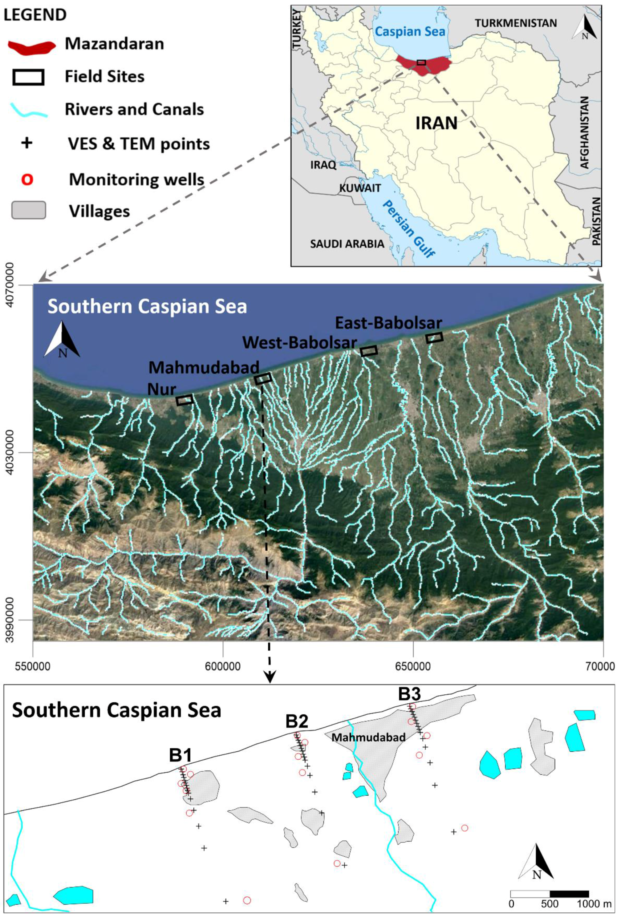
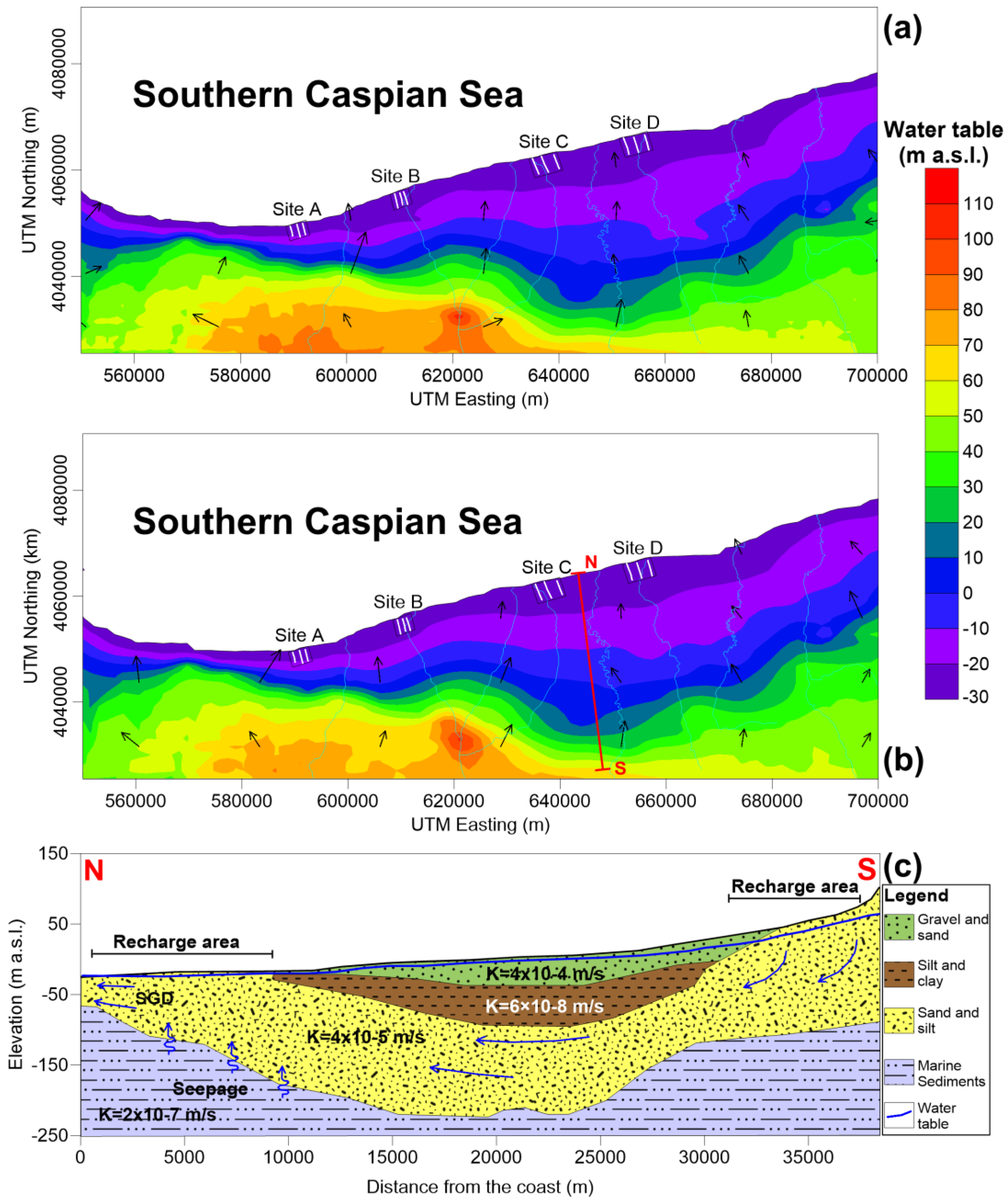
The Southern Caspian Sea area has a well-developed surface drainage network (Figure 1). The rivers are perennial since they are fed by the Elburz Mountains and their waters are used for agricultural purposes. From a hydrogeological point of view, this area consists of four hydrogeological units of unconsolidated sediments. The top one is a highly permeable unit consisting of sand and gravel calcareous materials. This unit constitutes the shallow unconfined aquifer and is limited to the upper alluvial plain. This unconfined aquifer gradually becomes thinner toward the north and disappears at a distance of 10 km from the Caspian Sea (Figure 2c). The second unit is an aquitard, composed of clay and silty-clay sediments, which impede the groundwater flux between the unconfined aquifer and the third hydrogeological unit. The latter is composed of gravel and fine- to medium-sized sands and forms the major aquifer of the area. The fourth hydrogeological unit is made of marine silty and sandy sediments saturated with paleo-brackish waters and behaves like a poorly transmissive hydrogeological unit with respect to the major aquifer of the area. In the study area (central panel of Figure 1), the aquifer is unconfined and formed by the third hydrogeological unit described above. The bedrock below the Quaternary sediments is generally found at a depth of more than 500 m [32].
With regard to the importance of the freshwater/saltwater interface location, different transects perpendicular to the coast were chosen according to the following principles: (i) different types of hydrogeological conditions had to be represented to account for lateral heterogeneities; (ii) a minimum of four monitoring wells had to be present along a flow line to allow for direct observations of the interface; (iii) site accessibility for field investigations and sampling had to be guaranteed.
Each of the four field sites (Nur, Mahmudabad, West-Babolsar, and East-Babolsar), covering an area of approximately 6 km2 (3 km along the shoreline × 2 km inland), include 3 transects spaced by a distance of 1500 m. Along each transect, 15 points were selected and investigated with both electrical resistivity sounding and electromagnetic sounding (bottom panel of Figure 1).
2.2. Groundwater Heads and Quality Data
The groundwater heads and quality data (TDS and major ions concentration) in agricultural and domestic wells were provided by the Ministry of Energy and by the Mazandaran Regional Water Company. Groundwater heads were measured in static conditions using an electric contact phreatimeter and converted into equivalent freshwater heads (Hf) to account for the variable density and salinity [33]. Groundwater heads measured in 340 wells were interpolated for May 2015 and October 2015 via ordinary kriging with a linear variogram, an anisotropy ratio of 2, and the nugget effect. A blank file was used to trim away the Caspian Sea from the contour map. A vector map was built on the interpolated grid to show the groundwater flow directions.
Chemical analysis of the water samples was carried out at the Mazandaran Regional Water Company, following an analytical procedure suggested by the American Public Health Association [34]. Specifically, Cl− was estimated using the standard AgNO3 titration method, Na+ was measured via the standard F-AAS method, and TDS was measured gravimetrically after heating at 105 °C for 24 h. The TDS map was interpolated by ordinary kriging with a linear variogram, an anisotropy ratio of 2, and the nugget effect. A blank file was used to trim away the Caspian Sea and the mountain area, where the groundwater quality data were sparse. To assess the accuracy of the TDS interpolation, open borehole logs of specific conductance (electrical conductivity normalized at 25 °C) were used to detect the saltwater interface in the monitoring wells located along the transects at each site. The downhole specific conductance data were acquired using a Solinst Levelogger LTC connected to a nylon wire. The freshwater/saltwater interface was set at a specific conductance of 4000 μS/cm, according to the classification scheme used in the Abu Dhabi Emirate [35]. Given that open borehole logs of specific conductance can be affected by biases with respect to the multi-level samplers’ data, the relative uncertainty of the observed saltwater interface was estimated to be around ±5% of the measured specific conductance as reported for a similar alluvial coastal aquifer [36].
2.3. Analytical Methods
The Ghyben–Herzberg analytical solution was the first to address the problem of the saltwater wedge. After that, many other solutions were presented [10,11,12,13]. The Verruijt analytical solution, widely accepted and used in recent years, has been employed in this study and is provided below:
In Equation (1), Z is the depth of the freshwater/saltwater interface below the water table (m); in Equation (2), Hf is the equivalent freshwater head (m); in Equation (3), X0 is the position of the freshwater/saltwater interface at the ground surface (positive values are from the shoreline toward the sea and negative values are inland from the shoreline). The terms of the equations are defined as follows:
where q is the groundwater specific discharge (m2/d); T is the aquifer transmissivity (m2/d), and i is the hydraulic gradient (-).
where β is a coefficient (-) accounting for the density contrast between freshwater (ρf = 1.0 gr/cm3) and saltwater (ρs = 1.013 gr/cm3).
where K is the hydraulic conductivity (m/d), and b is the aquifer thickness (m).
x is the distance (m) from the shoreline inland.
High K values lead to a shallow interface, while low K values give a deep interface [5], since the interface’s depth is related to aquifer lithological characteristics [37]. The values of T and K for each transect in the four sites were taken from the pumping tests performed by the Mazandaran Regional Water Company (see Supplementary Information).
2.4. Vertical Electric Sounding
The geo-electrical methods may contribute to an improved understanding of aquifer characteristics such as thickness of alluvium, particle size, bedrock depth, and an estimated depth of the freshwater/saltwater interface. Vertical electric sounding (VES) was performed using the Schlumberger configuration with a maximum current electrode separation of 150 m along each transect. An ABEM SAS 1000 Terrameter was used to obtain the apparent resistivity at each VES point. The data were interpreted by the conventional partial curve matching technique with two-layer master curves, in conjunction with an auxiliary point diagram. The data obtained from the VES were controlled using the software RESIST; in this way, true resistivity values were obtained. Drilling exploration borehole data were used to interpret the information derived from the VES, for all 12 transects.
2.5. Transient Electromagnetic Sounding
In order to determine the position of the freshwater/saltwater interface, the transient electromagnetic (TEM) method was used in the four field sites, in addition to the Verruijt equation and the VES method. In each field site, the TEM vertical profiles were calibrated along the transects using stratigraphic logs. The TEM method has the capability of achieving waves reflected from the underground layers to the ground surface at a very low electromagnetic frequency. This method can be performed using natural ground signals (inactive, such as magnetotelluric signals) or with artificial transmitter (active) in the near square or in the far square, using powerful military transmitters in the very low frequency (VLF) radio spectrum. The Developers Water Saraveyeh Company, combining the magnetotelluric signals and the VLF, created a tool with sensitive receivers that can acquire the low telluric turbulent waves as the minimum and maximum difference phase. The standard configuration was applied using a single-turn, 40 × 40 m2 transmitter loop with the receiver coil in the center of the loop. The transmitter of the TEM system had a maximum output of 3 A, resulting in a magnetic moment of 4800 m2A. The groundwater depth was determined using a brass rod. The electromagnetic square mobile receiver tool near this brass rod was able to determine the groundwater depth by taking the distance from the earth surface. The freshwater/saltwater interface was determined following the Fitterman and Stewart approach [38].
2.6. Methods’ Evaluation Using Statistical Operators
The reliability in capturing the position of the freshwater/saltwater interface with respect to the observed transition zone in the monitoring wells was assessed by calculating and comparing the value of the mean absolute error (MAE), the root mean square error (RMSE), the percent of bias (PBIAS), and the Wilcox index of agreement (d), for all the applied methods in the four study sites. PBIAS values were calculated as shown in [39]:
where Calcj is the calculated value corresponding to the observed one Obsj. The optimal value of PBIAS is 0.0, with low-magnitude values indicating an accurate model simulation. Positive values indicate model underestimation bias and negative values indicate model overestimation bias [38]. d values were calculated as shown in [40]:
where Obs is the mean value of the observed data. This statistical indicator can vary from 0 to 1; a computed value of 1 indicates a perfect agreement between the measured and predicted values, and 0 indicates no agreement at all [40].
3. Results and Discussion
3.1. Groundwater Flow Directions and Quality
From the spatial analysis of the Hf piezometric maps of May 2015 and October 2015 (Figure 2), a recharge area located in correspondence of the Elburz Mountain is visible in the southern part of the study area. In particular, in the western portion of the Amol–Ghaemshahr plain, the recharge area is not far away from the Caspian Sea and the hydraulic gradient is high, leading to a considerable groundwater discharge toward the sea; moving eastward, this pattern becomes less pronounced. The main rivers of the area supply water to the aquifer, since the bottom of the riverbeds are located always above the water table and the piezometric contours diverge from the main river courses. By comparison of the two maps (May versus October 2015), it is also evident that, at the end of the rainy season (the beginning of May), the groundwater table is higher than it is at the end of the summer season (the beginning of October), being +0.80 m on average with peaks in the mountains of +1.55 m. Given this transient behavior of the groundwater heads, the most exposed period to a possible salinization of groundwater resources is likely to be late summer–early autumn. For this reason, it was decided to perform the sampling campaign to record the TDS and the major ions in October 2015.
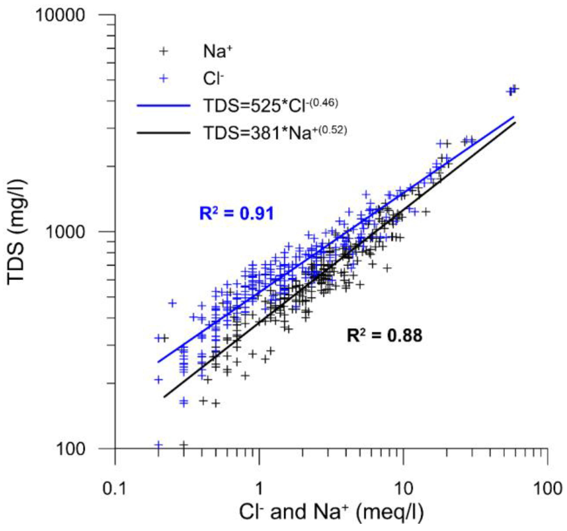
Before using TDS as a proxy of aquifer salinization, a scatter diagram correlating TDS versus Cl− and Na+ was plotted to demonstrate that these ions are governing the TDS trend, which is only marginally affected by other species (such as nitrates and sulfates), which are attributable to human activities. The high R2 (0.91 for Cl− and 0.88 for Na+) confirmed this hypothesis (Figure 3).
Figure 4 shows that most of the wells located in the Western portion of the study area are characterized by very fresh (0 < TDS < 1000 mg/L) and fresh waters (1000 < TDS < 2000 mg/L), while low brackish (2000 < TDS < 4000 mg/L) and medium brackish (4000 < TDS < 6000 mg/L) groundwater become more frequent in the eastern portion of the study area [34].
As reported by other authors [27,41], the aquifer system of the Amol–Ghaemshahr plain is characterized, especially in its eastern portion, by residual connate saline waters due to the eustatic variations in the Caspian Sea over the last 10,000 years [42]. Holding this, while Sites A, B, and C may essentially be affected by actual sweater intrusion, Site D may also be affected by autonomous salinization processes, exacerbated by the upconing of saline groundwater due to aquifer overexploitation. In general, defining a correct conceptual model of coastal aquifer salinization is vital not only for the sustainable water management but also for the implementation of saltwater intrusion mitigation strategies via coastal engineering systems [19]. When a dedicated network of multi-level samplers is not available, geophysical techniques can help to constrain the problem, as shown in the following sections.
3.2. Comparison of the Analytical Solution, VES, and TEM Results
In order to confirm the existence of groundwater discharge toward the sea, as suggested by the spatial analysis of the Hf piezometric maps of May 2015 and October 2015 (Figure 2), the location of the freshwater/saltwater interface at the ground surface (X0) was calculated by means of the Verruijt analytical solution in each transect (Table 1). Positive values stand for positions from the coast toward the sea, suggesting that a freshwater discharge is taking place, and negative values correspond to positions inland from the coast, suggesting that saltwater intrusion is occurring. Tidal fluctuations can affect the location of the freshwater/saltwater interface [19]; however, given that in the Southern Caspian Sea the maximum tidal range is just 21 cm with an average value of 10 cm [43], this effect was considered negligible.
All the calculated X0 values are positive, meaning that there is always a freshwater discharge toward the sea in the two available monitoring campaigns of May 2015 and October 2015 (Figure 2). In addition, X0 is always lower in October 2015, witnessing a decrease of freshwater discharge at the end of the summer months, as postulated by the analysis of the piezometric maps.
Accordingly, in the western transects (Nur and Mahmudabad sites), X0 is on average 12.05 m while in the eastern transects (West and East Babolsar) X0 is on average 1.08 m, testifying that, in the western part of the Amol–Ghaemshahr plain, the groundwater discharge toward the sea is higher (Figure 2).
The Verruijt analytical solution was also used to calculate the freshwater/saltwater interface for each transect of the four field sites. The analytical solution (AS) results were then compared with the VES and TEM interpolations, as well as with the monitoring campaign records of October 2015.
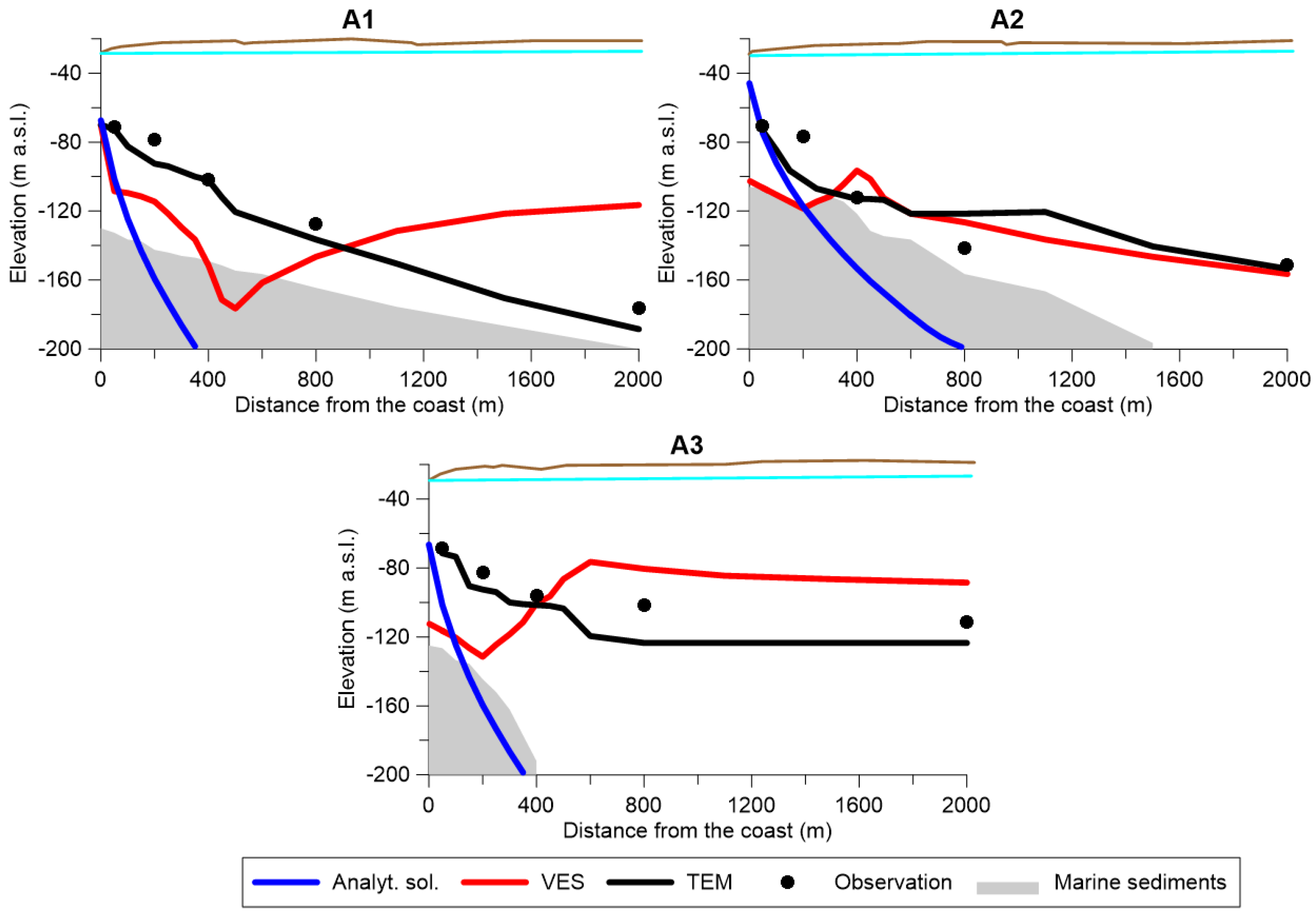
The average interface’s depths calculated with the AS were −215 m above sea level (ASL) in Nur (Site A in Figure 5), −178 m ASL in Mahmudabad (Site B in Figure 6), −104 m ASL in West-Babolsar (Site C in Figure 7), and −84 m ASL in East-Babolsar (Site D in Figure 8).
VES data were interpreted with the help of the boreholes’ log data available for each field site, then the freshwater/saltwater interface’s depth was determined in each transect. The average interface depths in Sites A, B, C and D were −119, −128, −91 and −65 m ASL, respectively (Figure 5, Figure 6, Figure 7 and Figure 8).
The same was done with the TEM data, and the average depths of the freshwater/saltwater interface in Sites A, B, C and D were calculated as −111, −108, −75 and −60 m ASL, respectively (Figure 5, Figure 6, Figure 7 and Figure 8).
More specifically, Figure 5 shows that, in Site A, the best method for locating the freshwater/saltwater interface is TEM, while the AS does not perform well. Likewise, the VES results are poor in A1 and A3, where the location of the interface with respect to the observed freshwater/saltwater interface in the monitoring wells is grossly overestimated in proximity to the shoreline and underestimated inland.
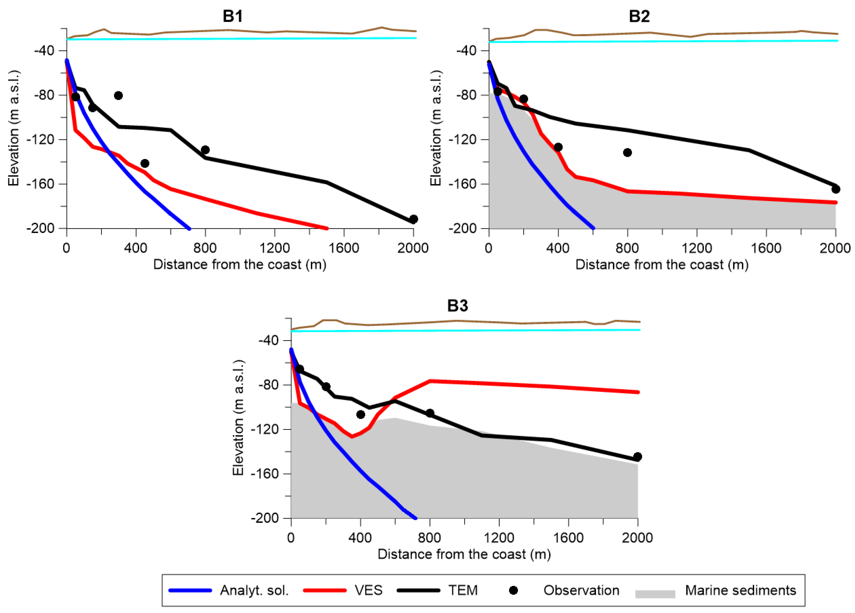
In Site B, the best method is still TEM (Figure 6), while AS provides satisfactory results only for Transect B1, overestimating the location of the freshwater/saltwater interface’s depth in the other two transects. The VES method seems to be less reliable, producing both overestimation and underestimation if compared with the records in the monitoring wells.
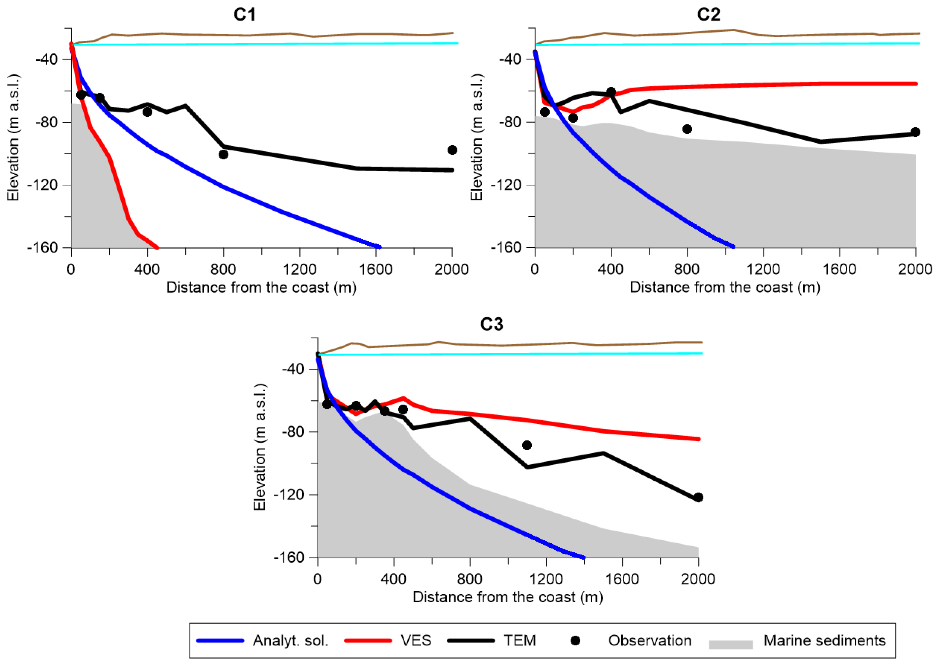
In Site C, the best method to capture the elevation of the transition zone is again TEM (Figure 7), while AS provides acceptable results only for Transect C1. The VES method is also not fully reliable, producing unrealistic results, above all moving inland.
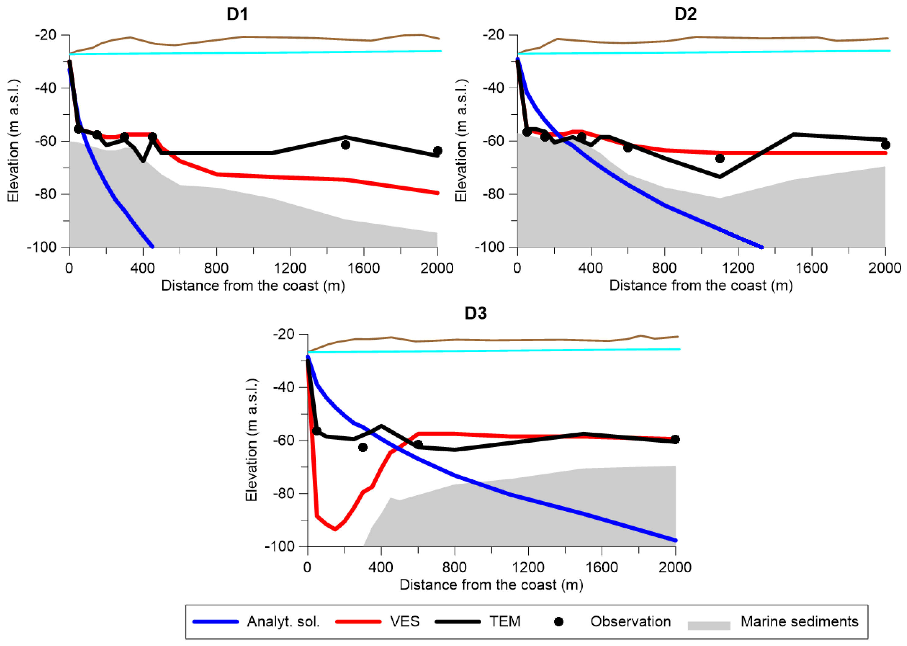
When describing the performance of the different methods in Site D, it is worth pointing out that AS cannot deal with the connate saline groundwater since it assumes simplified boundary conditions such as freshwater from inland and saltwater from the sea. For this reason, AS totally failed to correctly locate the saltwater/freshwater interface’s depth in Site D, where connate saline groundwater is most probably present even closer to the coast. The TEM is graphically the best method, although the VES in Site D slightly outperformed the other sites, especially in Transects D2 and D3.
In general, the results of the three methods applied in this study showed the following: (i) The AS method produced fair results in transects where the aquifer is characterized by a considerable thickness. In fact, the closer the saline aquitard is to the ground level (Sites C and D), the less accurate the interpolation. Moreover, the presence of sources of salinity other than actual seawater intrusion generates a high disturbance in the AS accuracy; (ii) In some transects, the VES method seems to be greatly influenced by the presence of the saline aquitard, often reproducing the saline aquitard/aquifer contact at a higher elevation than the actual one, rather than reproducing the saltwater/freshwater interface’s depth, as already raised by other studies [14,22]; (iii) The TEM method has proved to be the most reliable in capturing the freshwater/saltwater interface in all the configurations encountered in the transects. The values of the statistical indicators used to quantify the efficiency of each method in capturing the freshwater/saltwater interface for all the four field sites (A, B, C and D) are reported in Table 2.
In general, the AS method displays a very poor efficiency, with an MAE ranging between 37.3 and 58.6 m, and a d between 0.13 and 0.67, depending on the field site. This is due to local heterogeneities of T and K that influence the inland saltwater wedge extension. In fact, the use of K values higher than the mean ones derived from the pumping tests (see Supplementary Information) would considerably increase the saltwater/freshwater interface’s depth. However, to improve the efficiency of the AS method, a K increase of an order of magnitude would be needed. This is in contrast with the observed K variability that is comprised between 1.6 to 5.6 m/d in all sites (see Supplementary Information). Clearly, the choice of the K value is a key factor in the AS method, but the information on the aquifer properties at each site demonstrates that the AS method underestimates the extent of the saltwater wedge at all investigated sites. The VES method is also affected by large errors (5.9 < MAE < 30.7 m and 0.52 < d < 0.96) and cannot be safely employed to determine the freshwater/saltwater interface in complex geological settings, even if it becomes reliable under particular conditions. For instance, VES performance improves when a strong contrast between freshwater and saltwater concentrations exists, such as in Site D, where connate saline groundwater is most likely present. The TEM method outperforms the other two methods in all field sites (1.6 < MAE < 10.5 m and 0.96 < d < 0.99).
Interesting information is given by the PBIAS values that are nearly always negative, indicating a constant overestimation of the freshwater/saltwater interface’s depth, with all the three methods and in every field site. This could be due to a number of causes: local heterogeneities of the aquifer properties (e.g., fine-grained lenses, mineralogical composition of the sedimentary formations, and the degree of compaction), groundwater temperature variation with depth, which may be due to the cold groundwater flowing from the Elburz Mountain into the deepest portion of the aquifer, and the existence of upward fluxes from the deepest part of the aquifer toward the ground surface.
If Table 2 is analyzed with a greater focus on the performance of statistical indicators at the various sites rather than on the methods employed, it can be seen that, in Nur (Site A), the location of the freshwater/saltwater interface’s depth is highly uncertain, while in East-Babolsar (Site D) it is reliably identified. This behavior may be due to both the different hydrological boundary conditions characterizing the two sites and their contrasting salinity levels. In fact, while the Nur site is affected by a large seasonal variation in the groundwater flux, the boundary conditions in the East-Babolsar site are more stable. In addition, in this latter site, the presence of higher salinities may have enhanced the efficiency of the geophysical methods in distinguishing among freshwater and saltwater and thus in locating the interface that separates them.
4. Conclusions
Various methods exist for determining the position of the freshwater/saltwater interference, and each of them has different limitations that must be assessed and estimated. In this study, the Verruijt analytical solution (AS), the vertical electric soundings (VES), and the transient electromagnetic method (TEM) were employed, and their results were compared with the actual position of the transition zone retrieved within the monitoring wells located in a complex geological setting—namely, the one characterizing the Mazandaran Province (Southern Caspian Sea, Iran).
From a methodological point of view, it was demonstrated that the AS method is affected by a low accuracy in reconstructing the interface’s depth, which is in general grossly overestimated, with an increasing bias moving inland. The VES method is strongly affected by the saline aquitard/aquifer boundary’s depth. The TEM method showed the best fit to the observed data. Although the TEM method most suitably and cost-effectively locates the freshwater/saltwater interface in this area, the TEM method should not be employed alone; rather, it should be used in conjunction with other hydro-geophysical methods so as to better cope with subsurface uncertainties and thus ensure a high degree of reliability of the results [44].
From a water management perspective, this study emphasizes that the freshwater/saltwater interface in the area moves progressively closer to the ground level, moving from West to East within the coastal zone of the Amol–Ghaemshahr plain (approximately from −92 to −37 m BGL). This is due either to a large fresh groundwater discharge toward the Caspian Sea in the eastern zone, induced by the proximity to the coast of the Elburz Mountain’s recharge area, or to the upconing of the paleo brines in the western zone [27,41], which adds its effect to the actual seawater intrusion from the Caspian Sea. These natural phenomena are then exacerbated by the excessive withdrawal of groundwater from a dense network of wells used for domestic purposes and for irrigation, which in turn may worsen the picture by adding a polluted returned flow to the system. Given the fragile balance of the water resources in this area, and in view of the possible changes due to the fluctuation of the Caspian Sea level or to a variation of the recharge rates from the Elburz Mountains, it follows that a good management of the same cannot leave aside a detailed monitoring of the freshwater/saltwater interface’s depth. Accordingly, this study contributes in a broader sense to the characterization and monitoring of saltwater intrusion in coastal aquifers, where a network of multi-level samplers is not yet available, providing, for example, insightful information on where to install the monitoring wells, because a sound coastal management for the future will strongly depend on a sound knowledge of the actual salinization status.
Supplementary Materials
The following are available online at https://www.mdpi.com/2073-4441/10/4/348/s1.
Acknowledgments
The authors thank the Ministry of Energy and the Mazandaran Regional Water Company for the cooperation in providing the aquifer data and in conducting the field operations. Special thanks go to Mahdy Emadi, Management, and Budget Expert. No funds have been received for covering the costs to publish open access.
Author Contributions
Mohammad Golshan conceived and designed the experiments; Mohammad Golshan performed the experiments; Mohammad Golshan, Nicolò Colombani, and Micòl Mastrocicco analyzed the data; Nicolò Colombani, Micòl Mastrocicco, and Mohammad Golshan wrote the paper.
Conflicts of Interest
The authors declare no conflicts of interest.
References
- Barlow, P.M.; Reichard, E.G. Saltwater intrusion in coastal regions of North America. Hydrogeol. J. 2010, 18, 247–260. [Google Scholar] [CrossRef]
- Custodio, E.; Bruggeman, G.A. Groundwater Problems in Coastal Areas. Studies and Reports in Hydrology 45; UNESCO: Paris, France, 1987; pp. 15–88. ISBN 92-3-10241 5-9. [Google Scholar]
- Nowroozi, A.A.; Horrocks, S.B.; Henderson, P. Salt water intrusion into the freshwater aquifer in the eastern shore of Virginia: A reconnaissance electrical resistivity survey. J. Appl. Geophys. 1999, 42, 1–22. [Google Scholar] [CrossRef]
- Voss, C.I.; Souza, W.R. Variable density flow and solute transport simulation of regional aquifers containing a narrow freshwater-salt water transition zone. Water Resour. Res. 1987, 23, 1851–1866. [Google Scholar] [CrossRef]
- Essaid, H. A multilayered sharp interface model of coupled freshwater and salt water flow in coastal systems: Model development and application. Water Resour. Res. 1990, 26, 1431–1454. [Google Scholar] [CrossRef]
- Henry, H. Salt Intrusion into Fresh-Water Aquifers. J. Geophys. Res. 1959, 64, 1911–1919. [Google Scholar] [CrossRef]
- Van der Veer, P. Analytical solution for steady interface flow in a coastal aquifer involving phreatic surface with precipitation. J. Hydrol. 1976, 34, 1–11. [Google Scholar] [CrossRef]
- Badon-Ghyben, W. Nota in Verband Met de Voorgenomen Put Boring Nabij Amsterdam (Notes on the Probable Results of the Proposed Well Drilling Near Amsterdam). Kon. Inst. Ing. Tijdschr. Hague 1889, 21, 8–22. [Google Scholar]
- Herzberg, A. Die Wasserversorgung einiger Nordseebäder (The water supply on parts of the North Sea coast). J. Gasbeleucht. Wasserversorg. 1901, 44, 815–819. [Google Scholar]
- Glover, R.E. The pattern of fresh-water flow in a coastal aquifer. J. Geophys. Res. 1959, 64, 457–459. [Google Scholar] [CrossRef]
- Bear, J.; Dagan, J. Some exact solutions of interface problems by means of the hodograph method. J. Geophys. Res. 1964, 69, 1563–1572. [Google Scholar] [CrossRef]
- De Josselin de Jong, G. A many valued hodograph in an interface problem. Water Resour. Res. 1965, 1, 543–555. [Google Scholar] [CrossRef]
- Verruijt, A. An interface problem with a source and a sink in the heavy fluid. J. Hydrol. 1969, 8, 197–206. [Google Scholar] [CrossRef]
- Himi, M.; Tapias, J.; Benabdelouahab, S.; Salhi, A.; Rivero, L.; Elgettafi, M.; El Mandoure, A.; Stitou, J.; Casas, A. Geophysical characterization of saltwater intrusion in a coastal aquifer: The case of Martil-Alila plain (North Morocco). J. Afr. Earth Sci. 2017, 126, 136–147. [Google Scholar] [CrossRef]
- Colombani, N.; Osti, A.; Volta, G.; Mastrocicco, M. Impact of climate change on salinization of coastal water resources. Water Resour. Manag. 2016, 30, 2483–2496. [Google Scholar] [CrossRef]
- Mastrocicco, M.; Colombani, N.; Sbarbati, C.; Petitta, M. Assessing the effect of saltwater intrusion on petroleum hydrocarbons plumes via numerical modelling. Water Air Soil Pollut. 2012, 223, 4417–4427. [Google Scholar] [CrossRef]
- Oude Essink, G.H.P.; van Baaren, E.S.; de Louw, P.G.B. Effects of climate change on coastal groundwater systems: A modeling study in the Netherlands. Water Resour. Res. 2010, 46, W00F04. [Google Scholar] [CrossRef]
- Vandenbohede, A.; Hinsby, K.; Courtens, C.; Lebbe, L. Flow and transport model of a polder area in the Belgian coastal plain: Example of data integration. Hydrogeol. J. 2011, 19, 1599–1615. [Google Scholar] [CrossRef]
- Werner, A.D.; Bakker, M.; Post, V.E.A.; Vandenbohede, A.; Lu, C.; Ataie-Ashtiani, B.; Simmons, C.T.; Barry, D.A. Seawater intrusion processes, investigation and management: Recent advances and future challenges. Adv. Water Resour. 2013, 51, 3–26. [Google Scholar] [CrossRef]
- De Breuck, W.; De Moor, G. The water table aquifer in the eastern coastal area of Belgium. Hydrol. Sci. J. 1969, 14, 137–155. [Google Scholar] [CrossRef]
- Adepelumi, A.A.; Ako, B.D.; Ajayi, T.R.; Afolabi, O.; Omotoso, E.J. Delineation of saltwater intrusion into the freshwater aquifer of Lekki Peninsula, Lagos, Nigeria. Environ. Geol. 2009, 56, 927–933. [Google Scholar] [CrossRef]
- Choudhury, K.; Saha, D.K. Integrated Geophysical and Chemical Study of Saline Water Intrusion. Groundwater 2004, 42, 671–677. [Google Scholar] [CrossRef]
- Siemon, B.; Christiansen, A.V.; Auken, E. A review of helicopter-borne electromagnetic methods for groundwater exploration. Near Surf. Geophys. 2009, 7, 629–646. [Google Scholar] [CrossRef]
- Kontar, E.A.; Ozorovich, Y.R. Geo-electromagnetic survey of the fresh/salt water interface in the coastal southeastern Sicily. Cont. Shelf Res. 2006, 26, 843–851. [Google Scholar] [CrossRef]
- Leroy, S.A.G.; Marret, F.; Gibert, E.; Chalié, F.; Reyss, J.L.; Arpe, K. River inflow and salinity changes in the Caspian Sea during the last 5500 years. Quat. Sci. Rev. 2007, 26, 3359–3383. [Google Scholar] [CrossRef]
- Kosarev, A.N.; Yablonskaya, E.A. The Caspian Sea; SPB Academic Publishing: The Hague, The Netherlands, 1994; p. 259. ISBN 9051030886. [Google Scholar]
- Khairy, H.; Janardhana, M.R. Hydrogeochemical features of groundwater of semi-confined coastal aquifer in Amol–Ghaemshahr plain, Mazandaran Province, Northern Iran. Environ. Monit. Assess. 2013, 185, 9237–9264. [Google Scholar] [CrossRef] [PubMed]
- Gholami, V.; Yousefi, Z.; Rostami, H.Z. Modeling of ground water salinity on the Caspian southern coasts. Water Resour. Manag. 2010, 24, 1415–1424. [Google Scholar] [CrossRef]
- Colombani, N.; Osti, A.; Volta, G.; Mastrocicco, M. Misleading reconstruction of seawater intrusion via integral depth sampling. J. Hydrol. 2016, 536, 320–326. [Google Scholar] [CrossRef]
- Larsen, F.; Tran, L.V.; Van Hoang, H.; Tran, L.T.; Christiansen, A.V.; Pham, N.Q. Groundwater salinity influenced by Holocene seawater trapped in incised valleys in the Red River delta plain. Nat. Geosci. 2017, 10, 376–381. [Google Scholar] [CrossRef]
- Luo, X.; Kwok, K.L.; Liu, Y.; Jiao, J. A Permanent Multilevel Monitoring and Sampling System in the Coastal Groundwater Mixing Zones. Groundwater 2017, 55, 577–587. [Google Scholar] [CrossRef] [PubMed]
- Alavi, M. Tectonostratigraphic synthesis and structural style of the Alborz mountain system in northern Iran. J. Geodyn. 1996, 21, 1–33. [Google Scholar] [CrossRef]
- Post, V.E.A.; Kooi, H.; Simmons, C.T. Using hydraulic head measurements in variable-density ground water flow analyses. Groundwater 2007, 45, 664–671. [Google Scholar] [CrossRef] [PubMed]
- APHA Standard Methods for the Examination of Water and Waste Water, 20th ed.; American Public Health Association: Washington, DC, USA, 1995; p. 100.
- Mohamed, A.M.O. Arid Land Hydrogeology: In Search of a Solution to a Threatened Resource; CRC Press: Boca Raton, FL, USA, 2006; p. 170. ISBN 9780415411271. [Google Scholar]
- Mastrocicco, M.; Giambastiani, B.M.S.; Severi, P.; Colombani, N. The importance of data acquisition techniques in saltwater intrusion monitoring. Water Resour. Manag. 2012, 26, 2851–2866. [Google Scholar] [CrossRef]
- Anderson, W.P., Jr.; Evans, D.G.; Snyder, S.W. The effects of Holocene barrier-island evolution on water-table elevations, Hatteras Island, North Carolina, USA. Hydrogeol. J. 2000, 8, 390–404. [Google Scholar] [CrossRef]
- Fitterman, D.V.; Stewart, M.T. Transient electromagnetic sounding for groundwater. Geophysics 1986, 51, 995–1005. [Google Scholar] [CrossRef]
- Gupta, H.V.; Sorooshian, S.; Yapo, P.O. Status of automatic calibration for hydrologic models: Comparison with multilevel expert calibration. J. Hydrol. Eng. 1999, 4, 135–143. [Google Scholar] [CrossRef]
- Willmott, C.J. On the validation of models. Phys. Geogr. 1981, 2, 184–194. [Google Scholar]
- Motevalli, A.; Moradi, H.R.; Javadi, S.A. Comprehensive evaluation of groundwater vulnerability to saltwater up-coning and sea water intrusion in a coastal aquifer (case study: Ghaemshahr-juybar aquifer). J. Hydrol. 2018, 557, 753–773. [Google Scholar] [CrossRef]
- Naderi Beni, A.; Lahijani, H.; Mousavi Harami, R.; Arpe, K.; Leroy, S.A.G.; Marriner, N.; Berberian, M.; Andrieu-Ponel, V.; Djamali, M.; Mahboubi, A.; et al. Caspian sea-level changes during the last millennium: Historical and geological evidence from the south Caspian Sea. Clim. Past 2013, 9, 1645–1665. [Google Scholar] [CrossRef]
- Medvedev, I.P.; Kulikov, E.A.; Rabinovich, A.B. Tidal oscillations in the Caspian Sea. Oceanology 2017, 57, 360–375. [Google Scholar] [CrossRef]
- Comte, J.C.; Banton, O. Cross-validation of geo-electrical and hydrogeological models to evaluate seawater intrusion in coastal aquifers. Geophys. Res. Lett. 2007, 34. [Google Scholar] [CrossRef]
Figure 1.
The location of the field sites (Top panel): Nur (Site A), Mahmudabad (Site B), West-Babolsar (Site C), and East-Babolsar (Site D) within the Mazandaran Province (Central panel). As an example, the distribution of the VES and TEM points and of the monitoring wells are shown for the three transects of the Mahmudabad site (Bottom panel). In all the other transects, the configuration of the monitoring grid is analogous to the one reported here.

Figure 2.
The piezometric contour maps of Hf in m above sea level (ASL) in May 2015 (a) and October 2015 (b); the groundwater flow direction and magnitude are also reported (black arrows), along with the main river courses (cyan lines). The hydrogeological sketch (c) along the N–S transect (see panel (b) for location) is representative of the general hydrogeological setting of the study area; SGD stands for submarine groundwater discharge; mean K values are also indicated for each hydrogeological unit.

Figure 3.
The TDS versus Cl− and Na+ concentrations in 155 monitoring wells sampled in the field campaign of October 2015.
Figure 3.
The TDS versus Cl− and Na+ concentrations in 155 monitoring wells sampled in the field campaign of October 2015.

Figure 4.
The concentration contour map of TDS (mg/L) in October 2015 (a). The black crosses represent the 155 monitoring wells considered in the field campaign. TDS distribution emphasizes the limits among classes according to the scheme used in the Abu Dhabi Emirate [35]. The sketch (b) along the N–S transect (see panel (a) for location) is representative of the salinization processes affecting the study area; SWW stands for saltwater wedge.

Figure 5.
The elevation of the transition zone and extent of the saltwater wedge (colored lines) calculated via the Verruijt analytical solution, VES, and TEM methods in the Transects A1, A2 and A3 at the Nur site. The elevation of the transition zone observed in the selected monitoring wells is also shown. The ground elevation and the water table are plotted in brown and cyan, respectively.

Figure 6.
The elevation of the transition zone and extent of the saltwater wedge (colored lines) calculated via the Verruijt analytical solution, VES, and TEM methods in Transects B1, B2 and B3 at the Mahmudabad site. The elevation of the transition zone observed in the selected monitoring wells is also shown. The ground elevation and the water table are plotted in brown and cyan, respectively.

Figure 7.
The elevation of the transition zone and the extent of the saltwater wedge (colored lines) calculated via the Verruijt analytical solution, VES, and TEM methods in Transects C1, C2 and C3 at the West-Babolsar site. The elevation of the transition zone observed in the selected monitoring wells is also shown. The ground elevation and the water table are plotted in brown and cyan, respectively.

Figure 8.
The elevation of the transition zone and extent of the saltwater wedge (colored lines) calculated via the Verruijt analytical solution, VES, and TEM methods in Transects D1, D2 and D3 at the East-Babolsar site. The elevation of the transition zone observed in the selected monitoring wells is also shown. The ground elevation and the water table are plotted in brown and cyan, respectively.


Table 1.
The distance of the freshwater flux from the coast toward the sea (X0) in each section of the four field sites, for May 2015 and October 2015.
Table 1.
The distance of the freshwater flux from the coast toward the sea (X0) in each section of the four field sites, for May 2015 and October 2015.
| Site Name | Section | X0 (May 2015) m from the Coast | X0 (October 2015) m from the Coast |
|---|---|---|---|
| Site A (Nur) | A1 | 19.84 | 19.05 |
| A2 | 6.73 | 6.56 | |
| A3 | 18.77 | 17.65 | |
| Site B (Mahmudabad) | B1 | 8.85 | 8.69 |
| B2 | 12.37 | 12.14 | |
| B3 | 8.42 | 8.18 | |
| Site C (West-Babolsar) | C1 | 0.15 | 0.13 |
| C2 | 1.93 | 1.72 | |
| C3 | 0.94 | 0.81 | |
| Site D (East-Babolsar) | D1 | 2.95 | 2.15 |
| D2 | 1.04 | 0.97 | |
| D3 | 0.95 | 0.69 |
Table 2.
Statistical indicators quantifying the efficiency of the three methods AS, VES and TEM in locating the position of the freshwater/saltwater interface, with respect to the elevation of the transition zone measured within the observation wells.
Table 2.
Statistical indicators quantifying the efficiency of the three methods AS, VES and TEM in locating the position of the freshwater/saltwater interface, with respect to the elevation of the transition zone measured within the observation wells.
| Site Name | Method | MAE (m) | RMSE (m2) | PBIAS (m) | d (-) |
|---|---|---|---|---|---|
| Site A (Nur) | AS | 47.4 | 56.8 | −36.2 | 0.49 |
| VES | 30.7 | 35.6 | −12.2 | 0.72 | |
| TEM | 8.4 | 10.2 | −4.4 | 0.98 | |
| Site B (Mahmudabad) | AS | 37.3 | 44.2 | −33.1 | 0.67 |
| VES | 26.7 | 31.6 | −13.8 | 0.89 | |
| TEM | 10.5 | 12.3 | +1.6 | 0.96 | |
| Site C (West-Babolsar) | AS | 42.1 | 57.6 | −35.5 | 0.49 |
| VES | 27.1 | 41.2 | −12.6 | 0.52 | |
| TEM | 5.1 | 6.7 | +0.1 | 0.97 | |
| Site D (East-Babolsar) | AS | 58.6 | 83.9 | −96.1 | 0.13 |
| VES | 5.9 | 10.5 | −7.1 | 0.96 | |
| TEM | 1.6 | 2.2 | −0.5 | 0.99 |
© 2018 by the authors. Licensee MDPI, Basel, Switzerland. This article is an open access article distributed under the terms and conditions of the Creative Commons Attribution (CC BY) license (http://creativecommons.org/licenses/by/4.0/).
Share and Cite
MDPI and ACS Style
Golshan, M.; Colombani, N.; Mastrocicco, M. Assessing Aquifer Salinization with Multiple Techniques along the Southern Caspian Sea Shore (Iran). Water 2018, 10, 348. https://doi.org/10.3390/w10040348
AMA Style
Golshan M, Colombani N, Mastrocicco M. Assessing Aquifer Salinization with Multiple Techniques along the Southern Caspian Sea Shore (Iran). Water. 2018; 10(4):348. https://doi.org/10.3390/w10040348
Chicago/Turabian StyleGolshan, Mohammad, Nicolò Colombani, and Micòl Mastrocicco. 2018. "Assessing Aquifer Salinization with Multiple Techniques along the Southern Caspian Sea Shore (Iran)" Water 10, no. 4: 348. https://doi.org/10.3390/w10040348
Note that from the first issue of 2016, this journal uses article numbers instead of page numbers. See further details here.